Searching for Repeats, as an Example of Using the Generalized Ruzzo-Tompa Algorithm to Find Optimal Subsequences with Gaps

Abstract

Background

Some biological sequences contain subsequences of unusual composition, e.g., some proteins contain DNA binding domains, transmembrane regions, and charged regions; and some DNA sequences contain repeats. Requiring time linear in the length of an input sequence, the Ruzzo-Tompa (RT) Algorithm finds subsequences of unusual composition, using a sequence of scores as input and the corresponding “maximal segments” as output. (Loosely, maximal segments are the contiguous subsequences having greatest total score.) Just as gaps improved the sensitivity of BLAST, in principle gaps could help tune other tools, to improve sensitivity when searching for subsequences of unusual composition.

Results

Call a graph whose vertices are totally ordered a “totally ordered graph”. In a totally ordered graph, call a path whose vertices are in increasing order an “increasing path”. The input of the RT Algorithm can be generalized to a finite, totally ordered, weighted graph, so the algorithm then locates maximal segments, corresponding to increasing paths of maximal weight. The generalization permits penalized deletion of unfavorable letters from contiguous subsequences, so the generalized Ruzzo-Tompa algorithm can find subsequences with greatest total gapped scores. The search for inexact simple repeats in DNA exemplifies some of the concepts. For some limited types of repeats, RepWords, a repeat-finding tool based on the principled use of the Ruzzo-Tompa algorithm, performed better than a similar extant tool.

Conclusions

With minimal programming effort, the generalization of the Ruzzo-Tompa algorithm given in this article could improve the performance of many programs for finding biological subsequences of unusual composition.

Background

Repeats in Biological Sequences

Many eukaryotic genomes contain more repeats than protein-coding genes. For example, repeats occupy more than 50% of the human genome, whereas protein-coding sequences occupy only about 3% [1]. Although the terminology of repeats is not standardized, repeats are of two general types: (1) interspersed repeats, derived from transposons; and (2) simple repeats (also known as tandem repeats), which are inexact consecutive (or nearly consecutive) copies of a short oligonucleotide. Interspersed repeats are more common in the human genome [2], contributing to evolution in unexpected ways, notably by regulating mammalian genes [3–5], possibly because of epigenetic modifications [6–8]. On the other hand, simple repeats (sometimes known as microsatellites) are highly variable DNA sequences, usually less than 100 base pairs long, composed of short tandem repeats of 1–6 nucleotides. Typically, simple repeats have co-dominant inheritance, making them the markers of choice in a variety of applications, such as the characterization and certification of genetic materials in genetic mapping and breeding programs [9, 10].

Many repeat-finding tools recognize both interspersed and simple repeats. RepeatMasker, e.g., one of the most widely used tools for repeat identification [11], relies on local sequence alignment to compare genomic sequences with a library of known repeats [12]. The fact that both interspersed and simple repeats complicate sequence similarity searches has motivated a variety of tools for identifying and masking repeats [13–16]. Most tools, however, even ones for finding simple repeats, have an ad hoc basis. Our desire to provide mathematical foundations for finding simple repeats within biological sequences led us to generalize the Ruzzo-Tompa (RT) Algorithm, which finds ungapped subsequences of unusual composition [17]. Our generalization of the RT Algorithm finds gapped subsequences of unusual composition. A specialization of the generalization then finds gapped repeats within biological sequences.

The Ruzzo-Tompa Algorithm

The identification of unusual subsequences is a fundamental task in biological sequence analysis. Karlin and Altschul, e.g., assigned a score to each letter in a sequence, to search for contiguous subsequences with large total scores [18–20]. Their technique applies to proteins to find DNA-binding, transmembrane, or charged segments [21–23]. In a predecessor to the present article, Ruzzo and Tompa [17] give an example of how the technique was used to search for transmembrane segments of proteins. Transmembrane segments insert into the lipid bilayer of a cell membrane, so they tend to be more hydrophobic than the rest of the protein. Karlin and Brendel [24] assigned to each amino acid the corresponding score s(a) from the Kyte-Doolittle [25] hydrophobicity scale [26]. They then verified that contiguous high-scoring subsequences of the human β2-adrenergic receptor corresponded to known transmembrane domains. The Neyman-Pearson lemma [27] states, however, that log-odds scores are optimal statistics (according to a specific criterion), and so should improve on hydrophobicity scores. Accordingly, Karlin and Brendel derived log-odds scores s(a) from the empirical composition of amino acids within and outside of known transmembrane segments and then demonstrated improved identification and delimitation of the transmembrane segments in the β2-adrenergic receptor.

The Appendix describes the formal computational problem, but to describe the work of Ruzzo and Tompa [17] slightly less formally, let “:=” denote a definition. Consider any alphabet Λ (e.g., the nucleotides or amino acids) and any scoring function s : Λ ↦ R (e.g., the Kyte-Doolittle hydrophobicity scale above, which assigns a score s(a) to each amino acid a). Every amino acid sequence L := L₁ … L_n ∈ Λⁿ then corresponds to a numerical sequence x_i := s(L_i). Define a function S by S(0) := 0 and S(i) := x₁ + … + x_i (i= 1, 2, …, n). Our interest in subsequences motivates defining the segment [i, j] := {i, i+1, …, j} and the segmental score S[i, j] := S(j) − S(i) = x_i+1 + … + x_j. For brevity below, “score” always refers to a segmental score. Where necessary, we rely on context to disambiguate the (segmental) score S[i, j] and the function S(i). Below, “I” with various adornments such as primes, subscripts, etc., denotes a segment, e.g., if I = [i, j] then S(I) := S[i, j].

Ruzzo and Tompa [17] considered only scores S[i, j] of the form S[i, j] := S(j) − S(i), which we call “global scores”. The applications mentioned above demonstrate that global scores hold considerable biological interest, but our interest lies in other, more general types of scores for identifying unusual subsequences. Accordingly, let S̃(I) denote any segmental score, not necessarily a global score.

Let “⊂” denote strict inclusion of sets, and “⊃”, strict containment; so B ⊂ B′ iff (if and only if) B′ ⊃ B iff B ⊆ B′ and B ≠ B′. The segment I₀ satisfies “the Subsegment Property for S̃” iff S̃(I) < S̃(I₀) for every strict subsegment I ⊂ I₀. (We sometimes omit the qualification “for S̃” if S̃ is clear from context. Note that if I₀ contains no subsegments, it satisfies the Subsegment Property vacuously.) Intuitively, if S̃ = S is a global score derived from a function s : Λ ↦ R scoring a biological property, I₀ has more of the biological property than any of its proper subsegments. Now, consider any algorithm A whose input is a segment I, and whose output is a subsegment I₀ ⊆ I having the Subsegment Property and a positive score S̃(I₀) > 0, and maximizing the score S̃ over all I₀ ⊆ I. If there is more than one such I₀, A outputs one such I₀ arbitrarily; and if there is no such I₀, A outputs Ø.

From A, derive the following divide-and-conquer algorithm A^* : (0) set [i, j] ← [0, n]; (1) apply A to the input segment [i, j] to output a segment [i₀, j₀] ⊆ [i, j], and terminate A^* if the output of A is Ø; (2) otherwise, return to Step 1 recursively, inputting into A^* the segments to the left and right of [i₀, j₀], i.e., input both [i, j] ← [i, i₀] and [i, j] ← [j₀, j] into A^*. Call any segment in the output of A^* a “maximal segment within [0, n]”.

Ruzzo and Tompa pointed out that for a global score S̃ = S, just to read a set of values {S(i) : i ∈ [0, n]}, A^* generally requires O(n) time. At a minimum, then, A^* requires times typical of a divide-and-conquer algorithm: (1) worst-case time O(n²); and (2) expected time O(n log n). For a global score, Ruzzo and Tompa give an alternative to A^*, the RT Algorithm, which finds the maximal segments in linear O(n) time. The RT Algorithm can be found elsewhere [17]; the only detail relevant to the present article is that it inputs the values {S(i) : i ∈ [0, n]} sequentially.

Results

Statement of the General Theoretical Results

The RT Algorithm can be extended to solve a particular class of maximal path problems on weighted graphs. Call a graph G totally ordered iff its vertices are totally ordered. Without loss of generality, the vertices of a finite, totally ordered graph G can be labelled with the set [0, n] = {0, 1, …, n}, under the usual total ordering “<”. If G contains an edge from i to j (0 ≤ i < j ≤ n), denote the edge by (i, j), and for convenience below, direct the edge from i to j. Let R denote the real numbers, and associate a weight W(i, j) ∈ R ∪ {−∞} with each edge (i, j) of G. A (directed) path π from i₀ to i_k is a sequence of edges (i₀, i₁), …, (i_k−1, i_k) in G joining the vertices i₀ < … < i_k. (Because of the direction of the path’s edges, the path is “increasing”, according to the Abstract’s definition.) We write i ∈ π or (i, j) ∈ π to indicate that the vertex i or the directed edge (i, j) appears in the sequence of directed edges of π. Define the weight of π as $W(\pi ):={\sum }_{j=1}^{k}W\left(i_{j-1},i_j\right)$. For i < j, let Π[i, j] denote the set of directed paths from i to j. Consider the following segmental score, the “local score” Ŝ[i, j] := max{W(π) : π ∈ Π[i, j]}, with the convention that Ŝ[i, i] := 0. Define the corresponding global score S(i) = Ŝ[0, i]. To avoid trivialities, assume S(i) > −∞ for every i ∈ [0, n]. An edge weight −∞ cannot contribute to the global score S, so as will be seen, in practice, the weight −∞ is equivalent to omitting the corresponding edge from consideration.

In the present terminology, Ruzzo and Tompa [17] examined the local score, in the special case W(i − 1, i) = x_i, where W(i, j) = −∞ whenever j ≥ i + 2, so Ŝ[i, j] = S[i, j] = S(j) − S(i). To provide motivation for a more elaborate local score, consider a gap penalty g : N ↦ R, where N denotes the natural numbers. Let W(i − 1, i) := max{x_i, −g(1)} and W(i, j) := −g(j − i) for i, j ∈ [0, n] with j − i ≥ 2. The maximum defining W(i − 1, i) implicitly optimizes the edge between i − 1 and i as either a score or a gap of length 1. Then, the local score Ŝ[i, j] modifies the global score S[i, j] in Ruzzo and Tompa [17] by permitting gaps in the segment [i, j], and maximizing the total gapped score over all possible arrangements of the gaps.

Call a weighted, totally ordered graph G decreasing iff W(i, k) ≤ W(i, j) and W(i, k) ≤ W(j, k) for every i < j < k. In addition, the two segments [i₀, j₀] and [i₁, j₁] overlap internally iff j₀ ≠ i₁, j₁ ≠ i₀, and [i₀, j₀] ∩ [i₁, j₁] ≠ Ø. The Appendix proves the following theorem, which is our main result.

Theorem 1

In a finite, weighted, totally ordered, decreasing graph G with vertex set [0, n], consider the maximal segments corresponding to any local score Ŝ. Use the corresponding global scores {S(i) : i ∈ [0, n]} as input for the RT Algorithm, and call the corresponding output “RT-maximal segments”. Then: (1) all maximal segments for Ŝ within [0, n] are RT-maximal segments within [0, n], and vice versa; (2) for each maximal segment [i, j], Ŝ[i, j] = S(j) − S(i); and (3) if a segment I does not overlap internally with a maximal segment, then Ŝ(I) ≤ 0.

Remark

By computing the values S(i) (i = 0, 1, …, n) and using them as successive inputs to the RT Algorithm, the output contains all maximal segments for Ŝ and their scores, with a guarantee that the any segment not overlapping internally with a maximal segment has a non-positive score Ŝ. If the computation of each S(i) (i = 0, 1, …, n) requires O(1) (i.e., bounded) time (as in the application to repeats below), the RT Algorithm then outputs the maximal segments in time O(n), even though the weighted graph has O(n²) edges and O(n²) segments. Typically, given the score Ŝ[i, j] of a maximal segment [i, j], the standard technique of backtracking in a dynamic programming algorithm can then determine all paths from i to j having score Ŝ[i, j], if desired.

The Appendix proves Theorem 1.

A Specialization of the General Theoretical Results to Repeats

Let Λ be any alphabet (here, the nucleotide alphabet {A, C, G, T}), let s : Λ² ↦ R be any similarity matrix for Λ, and let the gap penalty g : N ↦ R be any non-decreasing function. (In applications, g is usually subject to additional restrictions, like positivity g > 0 and sublinearity g(i + j) ≤ g(i) + g(j); the affine gap penalty g(k) = Δ₀ + Δ₁k used below is common and satisfies both additional restrictions.) Consider any input sequence L := L_1−w … L_n ∈ Λ^n+w, where for convenience the initial index is the non-positive offset 1 − w. The “lagged scores” s(L_i−w, L_i) (i = 1, …, n) can detect simple repeats, as follows. As in the “Statement of the General Theoretical Results” above, consider a totally ordered weighted graph G with vertex set [0, n] and weights W(i − 1, i) := max{s(L_i−w, L_i), −g(1)} for 1 ≤ i ≤ n and W(i, j) := −g(j − i) for 0 ≤ i < j ≤ n (see Figure 1). Large scores Ŝ[i, j] correspond to inexact tandem repeats, where the directed edges with weights W(i − k, i) = −g(k) (k ≥ 2) correspond to gapping out k letter-pairs (L_j−w, L_j) with unfavorable scores s(L_j−w, L_j) (j = i − k + 1, …, i). For example, if s(a, b) = 1 for a = b, and s(a, b) = −∞ otherwise, gapless segments with positive scores correspond to exact tandem repeats of a single word of length w.

Figure 1. An example of a weighted, directed finite graph that induces a total order on its vertices, in an application to tandem repeats.

Figure 1 shows a sequence ACTACTGGTGG, an inexact tandem repeat of word-length w = 3. To score the repeat, shift the sequence by w = 3, and score the edges of length 1 (shown in red) with the score max {s(a,b), −g(1)}, e.g., with values as in the text. To permit gapping, score edges of length k > 1 with a length-dependent weight −g(k), e.g., as in the text. The edges with a black border indicate the maximally weighted path from left to right vertex, the gaps suggesting a mismatched segment within the repeat.

By construction, the weights W(i, j) are decreasing, so Theorem 1 states that the RT Algorithm applied to the global score S(j) = max{W(π) : π ∈ Π[0, j]} yields the maximal segments [i, j] for Ŝ and the corresponding scores Ŝ[i, j] = S(j) − S(i).

Implementation of the Program RepWords for Finding Repeats

Our computer program “RepWords” finds maximal segments associated with gapped repeats. RepWords is publicly available from the URL http://www.ncbi.nlm.nih.gov/CBBresearch/Spouge/html_ncbi/html/index/software.html#18. RepWords 1.0 is tuned to handle long sequences with minimal memory requirements, whereas RepWords 1.1 is faster, but requires more memory. The URL lists other differences between RepWords 1.0 and 1.1. All results and timing information presented here pertains to RepWords 1.1.

As a technical point, in a context analogous to Figure 1 and with a word-length w = 3, consider the sequence GGTGG. A maximal segment corresponding to the self-alignment

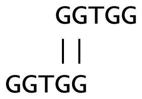
is of length ℓ = 2 < w. One could consider the entire five letters GGTGG as a repeat, but empirically, the ROC curves (Figure 3 below) improved if the repeat excluded the intermediate w − ℓ = 1 letters (e.g., the letter “T” above). Accordingly, if a maximal segment has length ℓ < w, the corresponding maximal subsequence has length 2ℓ and excludes the intermediate w − ℓ letters in the corresponding subsequence. On the other hand, if the maximal segment has length ℓ ≥ w, the corresponding maximal subsequence has length w + ℓ.

Figure 3. ROC curves comparing RepSeek and RepWords for different gap penalties.

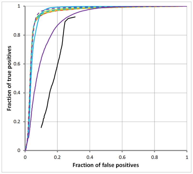
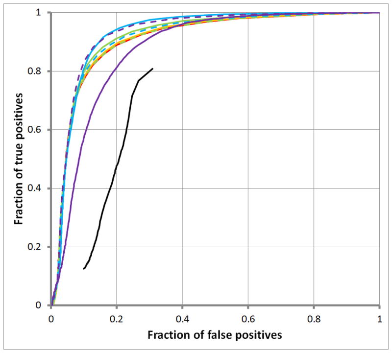
Figure 3A displays ROC curves for simple repeats; Figure 3B, for low complexity repeats. All repeats are classified according to RepeatMasker. The black curves show results for RepSeek with its default settings. RepWords (with the word-length w_max = 200) used the standard BLASTN match-mismatch scoring matrix s(a,b) = 2 for a =b and s(a,b) = −3 for a≠ b with a variety of gap penalties: g(k) = ∞ (solid red), so repeats are ungapped; g(k) = 5+k (solid orange); g(k) = 5 + 2k (dashed orange); g(k) = 3 + k (solid green); g(k) = 3 + 2k (dashed green); g(k) = 1 + k (blue);. g(k) = 1+ 2k (dashed blue); g(k) = k (solid purple); and g(k) = 2k (dashed purple).

Empirical Timing Results for RepWords and the Divide-and-Conquer Algorithm

Unless stated otherwise, all empirical results used the default BLASTN similarity matrix for the nucleotide alphabet {A, C, G, T} : s(a, b) = 2 for a = b, and s(a, b) = −3 otherwise.

To compare RepWords’ empirical computational times against the divide-and-conquer algorithm mentioned in the Background (adapted for repeat-finding), we generated random nucleotide sequences of different lengths under uniform background frequencies (0.25, 0.25, 0.25, 0.25) for the alphabet {A, C, G, T}. ROC curves (Figure 3 below) suggested that the BLASTN default gap penalty g(k) = 1 + k was superior to the BLASTN default gap penalty g(k) = 5 + 2k, so the timing tests used g(k) = 1 + k.

The timing results in Figure 2 show that for each repeat word-length w, RepWords determines the maximal segments in approximate time O(n); the divide-and-conquer algorithm, in approximate time O(n log n).

Figure 2. Computational time per letter in a sequence vs. the number of letters in the sequence.

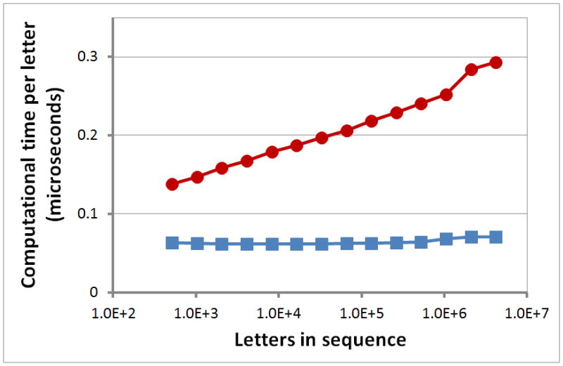
Figure 2 plots average timing results for random nucleotide sequences for the divide-and-conquer algorithm A^* in red circles; for the RT algorithm in blue squares.

ROC Curves for Repeat-Finding by RepWords and RepSeek

All empirical results involving real DNA were based on the full length of Human chromosome 19. In the following, percentages refer to the fraction of the length of Chromosome 19, 59,128,983 bases, of which 5.61% are Ns.

We adopted RepeatMasker [11] as our standard of truth for repeat-finding. Although the standard it provides is imperfect, no clearly superior standard is available. Under its default settings, RepeatMasker annotated repeats covering 54.55% of the length of Chromosome 19, classifying the repeats as follows: SINEs, 27.00%; LINEs, 12.97%; LTRs, 8.17%; DNA repeats, 2.04%; satellite repeats, 2.01%; simple repeats, 1.25%; low complexity repeats, 0.76%; and miscellaneous repeats, 0.37%.

Like RepWords, the repeat-finding program RepSeek [28] uses the lagged scores s(L_i−w, L_i) mentioned in “A Specialization of the General Theoretical Results to Repeats” above. The fact that the lagged scores have been used independently at least twice [29] suggests that they provide a natural method of finding simple repeats. RepSeek incorporates seed and gapped extension heuristics, however, unlike RepWords but somewhat like gapped BLAST [30].

We compared the empirical performance of RepWords and RepSeek by using ROC curves [31]. Various types of repeats called by our standard of truth, RepeatMasker, sometimes contain simple repeats within them. Given a particular repeat-type of interest, therefore: (1) any nucleotide base not in a RepeatMasker repeat was considered a negative (i.e., a non-repeat base); (2) any base within a RepeatMasker repeat of interest, a positive (i.e., a base of that type); and (3) because of overlapping repeats, all other bases were discarded from consideration, to avoid contamination of negatives with cryptic positives. As shown in Figure 3, RepWords decisively dominated RepSeek for finding simple repeats and low-complexity repeats. The Supplementary Information contains Figures S1A–S1F showing, however, that RepWords performed poorly on other types of repeats, either compared to RepSeek or in absolute terms (partly reflecting our intent, to develop a tool for finding simple inexact repeats).

Empirical Timing Results for RepWords and RepSeek

As the Methods describe, the use of RepSeek required splitting Chromosome 19 into pieces of approximately equal length, with 160 pieces corresponding to RepSeek’s best ROC performance in our hands. Piece #10 of the 160 pieces was taken arbitrarily as a typical piece, to time programs. The estimated CPU time RepSeek required for Piece #10 was about 262 sec (or about 11.7 hours for the entire chromosome). For comparison, RepWords should be slowest when its output contains all maximal segments, corresponding to a threshold score y = 1. Accordingly, for the timing results, we set y = 1. The ROC curves in Figure 3 suggest that RepWords’ repeat-finding performance is enhanced with the gap penalty g(k) = 1 + k, used accordingly for the timing results. On Piece #10 of Chromosome 19, RepWords output the union of all maximal segments for all word-lengths w up to the maximum word-length w_max = 10 in 0.13 sec CPU time; up to w_max = 20, in 0.18 sec; up to w_max = 100, in 0.66 sec; and up to w_max = 200, in 1.33 sec.

The Spectrum of Word-Lengths Composing a Repeat as Determined by RepWords

Figure 4 suggests that simple and low-complexity repeats are composed of a spectrum of word-lengths w. On one hand, the ROC curve for w_max = 10 rises most rapidly from the origin, suggesting that many simple and low-complexity repeats are dominated by short word-lengths w. The results displayed in Empirical Timing Results for RepWords and RepSeek

Figure 4. ROC curves comparing RepSeek and RepWords for different word-lengths.

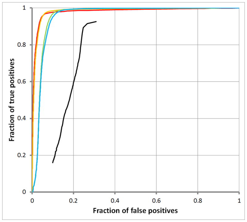
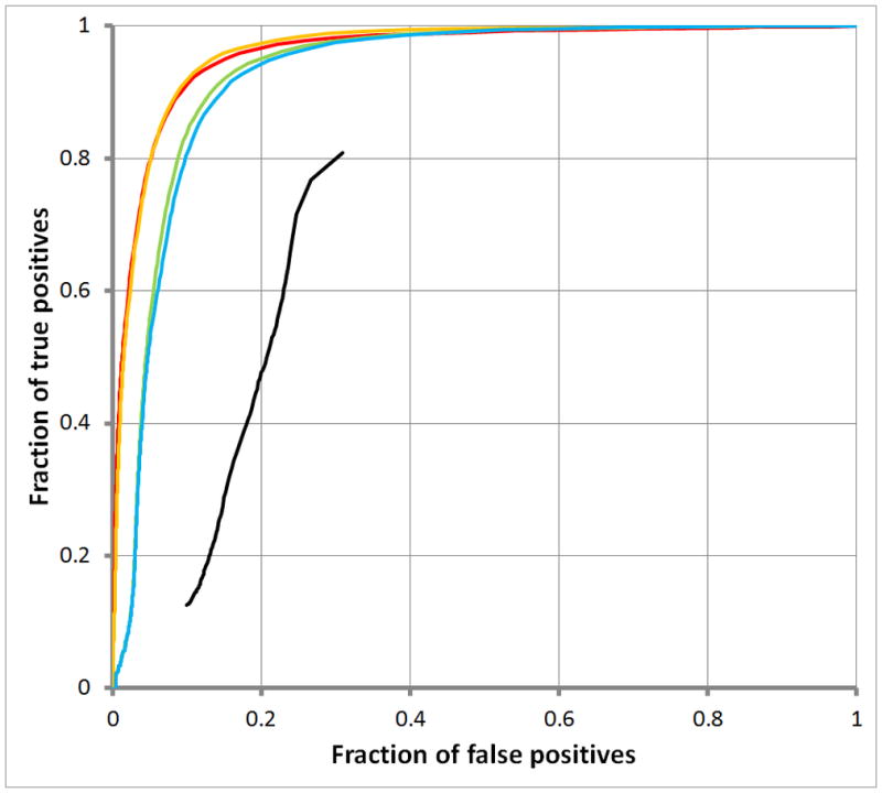
Figure 4A displays ROC curves for simple repeats; Empirical Timing Results for RepWords and RepSeek

Figure 4B, for low complexity repeats. The black curves show results for RepSeek with its default settings. RepWords used the standard BLASTN match-mismatch scoring matrix s(a, b) = 2 for a = b and s(a, b) = −3 for a ≠ b and the gap penalty g(k) = 1+ k with all word-lengths w up to the following maximum word-lengths: w_max = 10 (red); w_max = 20 (orange); w_max = 100 (green); and w_max = 200 (blue).

Figure 4 also suggest that decomposing repeats into a spectrum of word-lengths might be informative. Accordingly, Figure 5 decomposes two types of repeats into a spectrum of word-lengths w. On one hand, Figure 5A for SINE repeats shows abrupt rises in coverage, indicating that the corresponding word-lengths w contribute disproportionately to SINE repeats. On the other hand, Figure 5B for LINE repeats shows a steady rise, indicating an absence of word-lengths w contributing disproportionately to LINE repeats. (Corresponding plots for simple and low-complexity repeats were less striking, rising from 0.0 to 1.0 rapidly, indicating that the underlying spectrum of word-lengths w consists mostly of short word-lengths.)

Figure 5. Curves giving the spectrum of word-lengths underlying repeats up to word-length 1000.

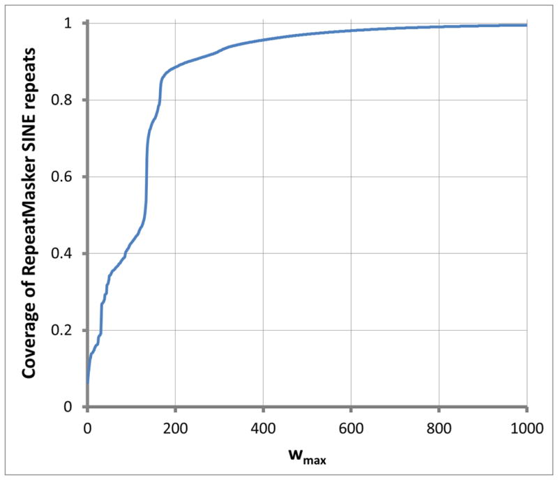
Figure 5A displays the curve for SINE repeats; Figure 5B, for LINE repeats. RepWords used the standard BLASTN match-mismatch scoring matrix s(a, b) = 2 for a = b and s(a, b) = −3 for a ≠ b and the gap penalty g(k) = 1 + k. The maximal segment score threshold chosen was y = 17. In the sense mentioned in the Methods, results are robust against the exact choice of y.

Discussion

This article generalizes the Ruzzo-Tompa algorithm for finding ungapped subsequences of unusual composition, effectively making it an algorithm for finding gapped subsequences of unusual composition. The generalization of the Ruzzo-Tompa (RT) algorithm holds the possibility of improving the performance of tools for finding biological subsequences of unusual composition, because minimal programming effort is now required to add and to tune gap penalties for individual biological applications.

In fact, our original desire was to develop a formal mathematical basis for finding simple repeats, which led us to generalize the RT Algorithm [17]. Unlike the ad hoc methods underlying most tools for finding repeats [14–16, 32, 33], but the generalized RT Algorithm provides our tool, RepWords, with a systematic approach generalizing some methods of repeat detection already extant in the literature [28, 29].

Figure 2 shows that although the more natural divide-and-conquer algorithm for locating subsequences of unusual composition requires time O(n log n) to find simple repeats, RepWords only requires time O(n) for each word-length w. Although RepWords searches individually for repeats of each word-length of interest, word-match heuristics (like those used in BLAST [30, 34, 35]) might accelerate simultaneous searches across different word-lengths w. We are currently investigating the incorporation of word-match heuristics into RepWords.

Within RepWords, Gotoh’s algorithm [36] calculates in constant time each of the global scores S(i) (i = 0, 1, …, n) as inputs for the RT Algorithm, limiting RepWords to affine gap penalties g(k) = Δ₀ + Δ₁k. Although affine gap penalties suffice for most repeat-finding applications, efficient algorithms are also available to calculate global scores for sub- or superlinear gap penalties g(k) [37–39]. Such algorithms can provide the corresponding input for the RT Algorithm, just as Gotoh’s algorithm did for affine gap penalties. In fact, the generalized RT Algorithm presented here requires only global scores S(i) as input; it even removes the need for any explicit algorithm to compute gapped segmental (local) scores Ŝ[i, j]! As exemplified by finding simple repeats within DNA sequences, therefore, this article provides a proof of principle, suggesting that the generalized RT Algorithm has broad implications for the methodical development of tools for finding subsequences of unusual composition.

Conclusions

This article generalizes the Ruzzo-Tompa (RT) Algorithm for finding ungapped subsequences of unusual composition, effectively making it an algorithm for finding gapped subsequences of unusual composition. With minimal programming effort, the generalization of the RT Algorithm holds the possibility of improving the performance of many tools for finding biological subsequences of unusual composition. As proof of principle in a specific case (perhaps not the simplest, but one reflecting the original motivation of the theory), the generalization is applied, to develop a tool for finding simple repeats. With repeat classes determined by using RepeatMasker as a gold standard, when finding the classes of simple and low-complexity repeats, the resulting tool (“RepWords”) performs well when compared to a tool with a similar but less general basis.

Methods

All computations were carried out on a 64-bit CentOS 5.8 operating system with 48G RAM and an Intel(R) Xeon(R) CPU X5660 (2.80GHz, 2 processors x 6 cores/2 threads).

The Ruzzo-Tompa Algorithm Applied to Finding Inexact Simple Repeats with Gaps Permitted

In the context of Theorem 1 and “A Specialization of the General Theoretical Results to Repeats”, consider the affine gap penalty g(k) = Δ₀ + Δ₁k common to many sequence applications. If Δ₁ ≥ 0, then the weights W(i, j) are decreasing, as required. The global score can be computed efficiently with the Gotoh affine gap algorithm, as follows [36]. Initialize with S₀ = 0 and I₀ = −∞. For j = 1, …, n,

$$\begin{array}{l}{S}_j=max\left\{S_{j-1},I_{j-1}\right\}+s\left(B_{j-w},B_j\right)\\ I_j=max\left\{S_{j-1}-{\mathrm{\Delta }}_0,I_{j-1}-min\left({\mathrm{\Delta }}_0,0\right)\right\}-{\mathrm{\Delta }}_1.\end{array}$$ (1)

(In most applications, Δ₀ ≥ 0, so the minimum in I_j is 0.)

The Gotoh affine gap algorithm computes S(j): = max{S_j, I_j} and the successive inputs S(i) (i ∈ [0, n]) are passed into the RT Algorithm.

ROC curves for RepSeek

To produce a ROC curve, the number of false positives predicted by a program must vary. Although the default mode of RepSeek has no free parameters, RepSeek does permit input of seed minimum length and repeat minimum score, similar to parameters in gapped BLAST [30]. As an option favorable to RepSeek’s performance, we varied the repeat minimum score parameter across its full range. When applied to the full length of Chromosome 19, RepSeek returned an error. To avoid computational problems, we therefore split Chromosome 19 into pieces and then combined the results from RepSeek. Figures display results from splitting Chromosome 19 into 160 pieces, corresponding to RepSeek’s best performance in our hands.

ROC curves for RepWords

All maximal segments [i, j] correspond to a local score Ŝ[i, j]. ROC curves for RepWords were generated by discarding all maximal segments with scores Ŝ[i, j] < y and then varying the threshold y.

Determining the Spectrum of Word-Lengths w Composing a Repeat-Type

Consider all bases in Chromosome 19 that RepeatMasker designated as, e.g., a SINE repeat. Call them “SINE bases”. Fix some arbitrary threshold y. Define RepWords’ coverage of RepeatMasker SINEs to be the fraction of SINE bases in at least one maximal subsequence (defined immediately above) whose word-length is no more than w_max and whose score is no less than y. Arbitrarily, we chose y = 17 as a threshold that includes most SINE bases for sufficiently large w_max. In Figure 5, an increase in y multiplies the coverage by an approximate constant less than 1.0, so (within limits) the results are robust against the choice of y, other than a change in the scale of the y-axis.

The Appendix

The Appendix section proves our main results, Theorem 2 and Theorem 3, through a series of technical lemmas. (The lemmas themselves are of very limited interest). Theorem 2 and Theorem 3 together imply Theorem 1 as a special case.

Sufficient Conditions for Disjoint Maximal Segments

Define (n):= [1, n] (a standard notation) and (n)₀:= [0, n], and fix a (segmental) score S̃. A segment I ⊆ I′ satisfies “the Supersegment Property within I′ for S̃” iff no supersegment I₀ ⊃ I such that I₀ ⊆ I′ has the Subsegment Property. (Thus, the Subsegment Property is intrinsic to a segment I, whereas the Supersegment Property has dependencies extrinsic to it.) A segment I₀ ⊆ I′ is an “RT-maximal segment within I′ for S̃” iff S̃(I₀) > 0 and I₀ has both the Subsegment Property and the Supersegment Property within I′ for S̃. The following omits “for S̃” if the score S̃ is clear from context; it sometimes omits the phrase “within I′” if I′ = [0, n].

For global scores, Ruzzo and Tompa proved that every RT-maximal segment is a maximal segment (i.e., one of the segments in the output of the divide-and-conquer algorithm A^*) and vice versa. To generalize their proofs to scores other than global scores, call S̃ an “RT score” iff it has two properties. The first is the Reverse Triangle Inequality: S̃[i, j] + S̃[j, k] ≤ S̃[i, k] whenever i < j < k. The second is the Positivity Property: if [i₀, j₀] has the Subsegment Property for S̃, then S̃[i₀, i] >0 and S̃[i, j₀] > 0 whenever i₀ < i < j₀. The proofs below use the convention that S̃[i, i]:= 0, to include the trivial inequalities S̃[i, i] + S̃[i, k] ≤ S̃[i, k] and S̃[i, k] + S̃[k, k] ≤ S̃[i, k] in the Reverse Triangle Inequality, thereby avoiding the separate analysis of boundary cases.

The present subsection essentially paraphrases the corresponding proofs in Ruzzo and Tompa [17] as a sequence of technical lemmas. In particular, the lemmas ensure that RT-maximal segments remain disjoint for general RT scores (Lemma 4 below), not just for global scores. Lemma 4 is crucial to the main result, Theorem 2, which asserts the equivalence of RT-maximal segments and maximal segments, demonstrating that the RT Algorithm and Algorithm A^* have equivalent outputs for an RT score. Lemma 1 shows that RT segmental scores generalize the notion of a global score.

Lemma 1

Every global score S is an RT score.

Proof

The Reverse Triangle Inequality is immediate (and reduces to equality for global scores). To prove the Positivity Property, if [i₀, j₀] has the Subsegment Property for S, then S[i, j] < S[i₀, j₀] for every [i, j] ⊂ [i₀, j₀]. The special case j = j₀ shows that S(i₀) < S(i) whenever i₀ < i < j₀. Similarly, the special case i = i₀ shows that S(j) < S(j₀) whenever i₀ < j < j₀. The definition S[i, j]:= S(j) − S(i) then proves the Positivity Property of S.

Lemma 2

For every score S̃, if S̃(I) > 0, then some I₀ ⊆ I has the Subsegment Property and a positive score S̃(I₀) > 0.

Proof

Either I itself has the Subsegment Property or else there is some I₁ ⊂ I such that S̃(I₁) ≥ S̃(I) > 0. Continue recursively. By the principle of infinite descent, the recursion terminates at some I₀ ⊂ I having the Subsegment Property (possibly vacuously) and a positive score S̃(I₀) > 0.

Lemma 3

Let S̃ be an RT score. Let I₀ = [i₀, j₀] ⊆ I′ have the Subsegment Property and a positive score S̃[i₀, j₀] > 0, and let I₁ = [i₁, j₁] be an RT-maximal segment within I′. If I₀ ∩ I₁ ≠Ø, then I₀ ⊆ I₁.

Proof

The Subsegment Property of I₀ and the Supersegment Property of I₁ within I′ exclude the possibility I₁ ⊂ I₀, so except for the case I₀ ⊆ I₁, there are only two symmetric cases remaining: (1) i₀ < i₁ ≤ j₀ < j₁ or (2) i₁ < i₀ ≤ j₁ < j₀. Using the Positivity Property, we eliminate Case 1 explicitly below; a symmetric argument eliminates Case 2.

In Case 1, i₀ < i ≤ j₁ implies i₀ < i ≤ j₀ or i₁ < i ≤ j₁ (or both), which leads to a contradiction, as follows. Whenever i₀ < i < j₀, the Subsegment Property of I₀ and its Positivity Property show that S̃[i₀, i] > 0. Moreover, S̃[i₀, j₀] > 0. Similarly, whenever i₁ < i ≤ j₁, the Reverse Triangle Inequality, the inequality S̃[i₀, i₁] > 0, and the Positivity Property of I₁ (or its positive score S̃[i₁, j₁] > 0) imply that S̃[i₀, i] ≥ S̃[i₀, i₁] + S̃[i₁, i] > 0. Thus, S̃[i₀, i] > 0 whenever i₁ < i ≤ j₁. By symmetry, S̃[j, j₁] > 0 whenever i₀ ≤ j < j₁. Consequently, for every [i, j] ⊂ [i₀, j₁],

$$\stackrel{\sim }{S}[i_0,j_1]\ge \stackrel{\sim }{S}[i_0,i]+\stackrel{\sim }{S}[i,j]+\stackrel{\sim }{S}[j,j_1]>\stackrel{\sim }{S}[i,j].$$ (2)

Thus, [i₀, j₁] has the Subsegment Property, which contradicts the Supersegment Property of [i₁, j₁] ⊂ [i₀, j₁] within I′. As stated above, the only remaining possibility is I₀ ⊆ I₁.

Lemma 4

For an RT score S̃, if I₀ and I₁ are distinct RT-maximal segments within I′, they are disjoint.

Proof

Every RT-maximal segment within I′ has the Subsegment Property. Lemma 3 implies, therefore, if I₀ ∩ I₁ ≠ Ø, then both I₀ ⊆ I₁ and I₁ ⊆ I₀, so I₀ = I₁.

Lemma 5

For an RT score S̃, let [i₀, j₀] be RT-maximal within [i, j]. Then, (1) I₁ ⊆ [i, i₀] is RT-maximal within [i, j] iff I₁ is RT-maximal within [i, i₀], and (2) I₁ ⊆ [j₀, j] is RT-maximal within [i, j] iff I₁ is RT-maximal within [j₀, j].

Proof

We prove Assertion (1) explicitly; Assertion (2) then follows by a symmetric argument. All hypotheses and conclusions state that I₁ has the Subsegment Property and a positive score, so the proof considers only the relevant Supersegment Properties. (1. ⇒) If no supersegment I₂ such that I₁ ⊂ I₂ ⊆ [i, j] has the Subsegment Property, then a fortiori, no supersegment I₂ such that I₁ ⊂ I₂ ⊆ [i, i₀] has the Subsegment Property. (1. ⇐) If I₁ were RT-maximal within [i, i₀] but not within [i, j], then I₁ ⊂ I₂, where I₂ has the Subsegment Property, S(I₂) > S(I₁) > 0, and I₂ ∩ [i₀, j₀] ≠ Ø. By Lemma 3, [i₀, j₀] cannot be maximal within [i, j], a contradiction.

Two segments [i₀, j₀] and [i₁, j₁] overlap internally iff j₀ ≠ i₁, j₁ ≠ i₀, and [i₀, j₀] ∩ [i₁, j₁] ≠ Ø.

Theorem 2

For any RT score S̃, (1) if a segment I has a positive score S(I) > 0, then it overlaps internally with a RT-maximal segment; and (2) all maximal segments within [0, n] are RT-maximal segments within [0, n], and vice versa.

Proof of Conclusion (1)

By Lemma 2, any segment with a positive score contains a segment having the Subsegment Property and a positive score. Thus, it overlaps internally with an RT-maximal segment.

Proof of Conclusion (2)

Given input I, Algorithm A outputs an RT-maximal segment I₀ within I (I₀ has the Subsegment Property and a positive score, and no segment within I has a strictly larger score than I₀, so no supersegment I′ ⊃ I₀ within I can have the Subsegment Property). Inductive application of Lemma 5 shows that whenever A finds an RT-maximal segment within I ⊆ [0, n], in fact it finds another RT-maximal segment within [0, n]. Thus, A^* outputs only segments RT-maximal in [0, n], so every maximal segment is an RT-maximal segment. Lemma 4 shows that A^* terminates only after all RT-maximal segments appear in its output, so every RT-maximal segment is also a maximal segment.

A Path Optimization with Disjoint Maximal Segments

The Background introduced the local score Ŝ[i, j]:= max{W(π): π ∈ Π[i, j]}, with the convention that Ŝ[i, i] :=0. Again, a sequence of technical lemmas precedes the main result, Theorem 3 and its Remark, which together assert that the maximal segments of Ŝ and S, along with their scores, are the same. Before proceeding, let us list some properties of any local score Ŝ.

Lemma 6

For any local score Ŝ, the following properties hold: (1) the extended Reverse Triangle Property, that Ŝ[i, j] + Ŝ[j, k] ≤ Ŝ[i, k] whenever 0 ≤ i ≤ j ≤ k ≤ n; (2) the Edge Maximization Property, that Ŝ[i, j] + W (j, j′) + Ŝ [j′, k] ≤ Ŝ[i,k] whenever [j, j′] ⊆ [i, k] ⊆ [0, n]; and (3) the Internal Point Maximization Property: if j ∈ π for any π ∈ Π[i, k] satisfying W(π) = Ŝ[i,k], then Ŝ[i, k] = Ŝ[i, j] + Ŝ[j, k].

Proof

Any cases not handled in the proof follow implicitly from the convention that Ŝ[i, i] :=0. (1) The Reverse Triangle Inequality holds whenever 0 ≤ i < j < k ≤ n, because both sides maximize path weights over paths π from i to k, but the one on the left includes the extra restriction that j ∈ π. (2) The Edge Maximization Property holds whenever [j, j′] ⊆ [i, k] ⊆ [0, n], because both sides maximize path weights over paths π from i to k, but the one on the left includes the extra restriction that (j, j′) ∈ π. (3) The Internal Point Maximization Property holds whenever i < j < k because maximizing path weights over the segments [i, j] and [j, k] separately cannot improve on the maximum weight W(π) = Ŝ[i,k]

As a special case of the extended Reverse Triangle Inequality, for every 0 ≤ i ≤ j ≤ n,

$$\widehat{S}[i,j]\le \widehat{S}[0,j]-\widehat{S}[0,i]=S(j)-S(i)=S[i,j].$$ (3)

Lemma 6 specializes to produce other statements involving the global score S; the following uses the implicit specializations without comment. Lemma 6 shows that the Reverse Triangle Inequality follows from the definition of Ŝ. The Positivity Property for Ŝ, however, requires an additional restriction on W(i, j). Call the weights “decreasing” iff W (i, k) ≤ W (i, j) and W (i, k) ≤ W (j, k) for every 0≤ i < j < k ≤ n.

Lemma 7

For decreasing weights, Ŝ is an RT score.

Proof

To prove that Ŝ has the Positivity Property, let [i₀, j₀] have the Subsegment Property for Ŝ, i.e., Ŝ[i, j] < Ŝ[i₀, j₀] for every [i, j] ⊂ [i₀, j₀]. Let W(π) = Ŝ[i₀, j₀] for π ∈ Π[i₀, j₀], to prove by contradiction that Ŝ[i₀, i] > 0 whenever i₀ < i < j₀.

If not, then Ŝ[i₀, i] ≤ 0 for some i satisfying i₀ < i < j₀. If i ∈ π, the Internal Point Maximization Property in Lemma 6 yields

$$\widehat{S}[i_0,j_0]=\widehat{S}[i_0,i]+\widehat{S}[i,j_0]\le \widehat{S}[i,j_0],$$ (4)

contradicting the Subsegment Property of [i₀, j₀], thereby implying i ∉ π. Then, however, (i′, j′) ∈ π for some i₀ ≤ i′ < i < j′ ≤ j₀. Because W(i′, j′) ≤ W (i′, i),

$$\begin{array}{l}\widehat{S}[i_0,j_0]=\widehat{S}[i_0,i^{\prime }]+W(i^{\prime },j^{\prime })+\widehat{S}[j^{\prime },j_0]\\ \le \widehat{S}[i_0,i^{\prime }]+W(i^{\prime },i)+\widehat{S}[j^{\prime },j_0]\\ \le \widehat{S}[i_0,i]+\widehat{S}[j^{\prime },j_0],\end{array}$$ (5)

where the equality follows from the Edge Maximization Property in Lemma 6; the first inequality, from decreasing weights; and the final inequality, from a degenerate case of the Edge Maximization Property. If j′ = j₀, then Ŝ[i₀, j₀] ≤ Ŝ[i₀, i]; otherwise Ŝ[i₀, i] ≤ 0 implies Ŝ[i₀, j₀] ≤ Ŝ[j′, j₀] for j′ < j₀. In either case, Eq (5) contradicts the Subsegment Property of [i₀, j₀]. Thus, Ŝ[i₀, i] > 0 whenever i₀ < i < j₀.

A symmetric argument yields Ŝ[i, j₀] > 0 whenever i₀ < i < j₀. Thus, Ŝ is an RT score.

Now, we show that for decreasing weights, the RT-maximal segments for the local score Ŝ and the global score S are in fact identical. Recall throughout the proofs that Lemma 6 has implications for S(j) = Ŝ[0, j].

Lemma 8

For decreasing weights, given any segment [i₀, j₀], if S(i₀) < S (i) whenever i₀ < i ≤ j₀, then Ŝ[i₀, i] = S(i) − S(i₀) > 0 whenever i₀ < i ≤ j₀.

Proof

Let W(π) = S(i) for π ∈ Π[0,i] and i₀ < i ≤ j₀. Let us prove that i₀ ∈ π, so the Internal Point Maximization Property in Lemma 6 then yields the required conclusion. If i₀ = 0, then i₀ ∈ π. Otherwise, if i₀ ∉ π, then some (i′, j′) ∈ π, where 0 ≤ i′ < i₀ < j′ ≤ i ≤ j₀. A degenerate case of the Internal Edge Maximization Property shows that S(i′) + W(i′,i₀) ≤ S(i₀), so

$$\begin{array}{l}S(j^{\prime })=S(i^{\prime })+W(i^{\prime },j^{\prime })\\ \le S(i^{\prime })+W(i^{\prime },i_0)\le S(i_0)<S(j^{\prime }),\end{array}$$ (6)

because W(i′, j′) ≤ W(i′, i₀). The contradiction proves i₀ ∈ π, so Lemma 8 follows.

Theorem 3

For decreasing weights, [i₀, j₀] has the Subsegment Property for S iff it has the Subsegment Property for Ŝ. Moreover, any segment [i₀, j₀] possessing the Subsegment Properties for S and Ŝ satisfies Ŝ[i₀, j₀] = S[i₀, j₀] = S(j₀) − S(i₀).

Remark

Theorem 3 implies the Supersegment Properties for S and Ŝ are also equivalent, so every RT-maximal segment for S is also a RT-maximal segment for Ŝ, and vice versa. Both Ŝ and (more particularly) S are RT scores, so Theorem 2 pertains.

Proof

(⇒) If [i₀, j₀] has the Subsegment Property for S, then S[i, j] < S[i₀, j₀] for every [i, j] ⊂ [i₀, j₀]. An examination first of [i, j₀] ⊂ [i₀, j₀] and then of [i₀, i] ⊂ [i₀, j₀] shows that S(i₀) < S(i) < S(j₀) whenever i₀ < i < j₀. Thus, for every [i, j] ⊂ [i₀, j₀], because S(i) + Ŝ[i, j] ≤ S(j),

$$\begin{array}{l}\widehat{S}[i,j]\le S(i)+\widehat{S}[i,j]-S(i_0)\\ \le S(j)-S(i_0)\le S(j_0)-S(i_0)=\widehat{S}[i_0,j_0],\end{array}$$ (7)

where Lemma 8 justifies the final equality. Because either the first or the third inequality is strict, Eq (7) implies the Subsegment Property for Ŝ within [i₀, j₀].

(⇐) If [i₀, j₀] has the Subsegment Property for Ŝ, then the Positivity Property shows that Ŝ[i₀, i] > 0 and Ŝ[i, j₀] > 0 whenever i₀ < i < j₀. Eq (3) then yields S[i₀,i] > 0 and S[i, j₀] > 0, whenever i₀ < i < j₀. Thus, S(i₀) < S(i) < S (j₀) for every i satisfying i₀ < i < j₀, implying

$$S[i_0,j_0]=S(j_0)-S(i_0)>S(j)-S(i)=S[i,j]$$ (8)

for every [i, j] ⊂ [i₀, j₀], i.e., [i₀, j₀] has the Subsegment Property for S.

Together, Theorem 2 and Theorem 3 imply Theorem 1.

References

- 1.Lander ES, Linton LM, Birren B, Nusbaum C, Zody MC, Baldwin J, Devon K, Dewar K, Doyle M, FitzHugh W, et al. Initial sequencing and analysis of the human genome. Nature. 2001;409(6822):860–921. doi: 10.1038/35057062. [DOI] [PubMed] [Google Scholar]
- 2.Smit AF. Interspersed repeats and other mementos of transposable elements in mammalian genomes. Curr Opin Genet Dev. 1999;9(6):657–663. doi: 10.1016/s0959-437x(99)00031-3. [DOI] [PubMed] [Google Scholar]
- 3.Feschotte C. Transposable elements and the evolution of regulatory networks. Nat Rev Genet. 2008;9(5):397–405. doi: 10.1038/nrg2337. [DOI] [PMC free article] [PubMed] [Google Scholar]
- 4.Marino-Ramirez L, Jordan IK. Transposable element derived DNaseI-hypersensitive sites in the human genome. Biol Direct. 2006;1:20. doi: 10.1186/1745-6150-1-20. [DOI] [PMC free article] [PubMed] [Google Scholar]
- 5.Marino-Ramirez L, Lewis KC, Landsman D, Jordan IK. Transposable elements donate lineage-specific regulatory sequences to host genomes. Cytogenet Genome Res. 2005;110(1–4):333–341. doi: 10.1159/000084965. [DOI] [PMC free article] [PubMed] [Google Scholar]
- 6.Huda A, Marino-Ramirez L, Jordan IK. Epigenetic histone modifications of human transposable elements: genome defense versus exaptation. Mob DNA. 2010;1(1):2. doi: 10.1186/1759-8753-1-2. [DOI] [PMC free article] [PubMed] [Google Scholar]
- 7.Huda A, Marino-Ramirez L, Landsman D, Jordan IK. Repetitive DNA elements, nucleosome binding and human gene expression. Gene. 2009;436(1–2):12–22. doi: 10.1016/j.gene.2009.01.013. [DOI] [PMC free article] [PubMed] [Google Scholar]
- 8.Huda A, Tyagi E, Marino-Ramirez L, Bowen NJ, Jjingo D, Jordan IK. Prediction of transposable element derived enhancers using chromatin modification profiles. PLoS One. 2011;6(11):e27513. doi: 10.1371/journal.pone.0027513. [DOI] [PMC free article] [PubMed] [Google Scholar]
- 9.Simbaqueba J, Sanchez P, Sanchez E, Nunez Zarantes VM, Chacon MI, Barrero LS, Marino-Ramirez L. Development and characterization of microsatellite markers for the Cape gooseberry Physalis peruviana. PLoS One. 2011;6(10):e26719. doi: 10.1371/journal.pone.0026719. [DOI] [PMC free article] [PubMed] [Google Scholar]
- 10.Garzon-Martinez GA, Zhu I, Landsman D, Barrero LS, Marino-Ramirez L. The Physalis peruviana leaf transcriptome: assembly, annotation and gene model prediction. BMC Genomics. 2012;13(1):151. doi: 10.1186/1471-2164-13-151. [DOI] [PMC free article] [PubMed] [Google Scholar]
- 11.RepeatMasker. at http://repeatmasker.org.
- 12.Jurka J, Kapitonov VV, Pavlicek A, Klonowski P, Kohany O, Walichiewicz J. Repbase Update, a database of eukaryotic repetitive elements. Cytogenet Genome Res. 2005;110(1–4):462–467. doi: 10.1159/000084979. [DOI] [PubMed] [Google Scholar]
- 13.Wootton JC, Federhen S. Analysis of compositionally biased regions in sequence databases. Methods Enzymol. 1996;266:554–571. doi: 10.1016/s0076-6879(96)66035-2. [DOI] [PubMed] [Google Scholar]
- 14.Benson G. Tandem repeats finder: a program to analyze DNA sequences. Nucleic Acids Res. 1999;27(2):573–580. doi: 10.1093/nar/27.2.573. [DOI] [PMC free article] [PubMed] [Google Scholar]
- 15.Morgulis A, Gertz EM, Schaffer AA, Agarwala R. WindowMasker: window-based masker for sequenced genomes. Bioinformatics. 2006;22(2):134–141. doi: 10.1093/bioinformatics/bti774. [DOI] [PubMed] [Google Scholar]
- 16.Frith MC. A new repeat-masking method enables specific detection of homologous sequences. Nucleic Acids Res. 2011;39(4):e23. doi: 10.1093/nar/gkq1212. [DOI] [PMC free article] [PubMed] [Google Scholar]
- 17.Ruzzo WL, Tompa M. A linear time algorithm for finding all maximal scoring subsequences. Proc Int Conf Intell Syst Mol Biol. 1999:234–241. [PubMed] [Google Scholar]
- 18.Karlin S, Altschul SF. Methods for assessing the statistical significance of molecular sequence features by using general scoring schemes. Proc Natl Acad Sci U S A. 1990;87 (6):2264–2268. doi: 10.1073/pnas.87.6.2264. [DOI] [PMC free article] [PubMed] [Google Scholar]
- 19.Karlin S, Dembo A, Kawabata T. Statistical Composition of High-Scoring Segments From Molecular Sequences. Ann Stat. 1990;18(2):571–581. [Google Scholar]
- 20.Karlin S, Altschul SF. Applications and statistics for multiple high-scoring segments in molecular sequences. Proc Natl Acad Sci U S A. 1993;90(12):5873–5877. doi: 10.1073/pnas.90.12.5873. [DOI] [PMC free article] [PubMed] [Google Scholar]
- 21.Brendel V, Dohlman J, Blaisdell BE, Karlin S. Very Long Charge Runs In Systemic Lupus Erythematosus-Associated Autoantigens. Proc Natl Acad Sci U S A. 1991;88(4):1536–1540. doi: 10.1073/pnas.88.4.1536. [DOI] [PMC free article] [PubMed] [Google Scholar]
- 22.Karlin S, Brendel V. Patchiness and Correlations In DNA Sequences. Science. 1993;259(5095):677–680. doi: 10.1126/science.8430316. [DOI] [PubMed] [Google Scholar]
- 23.Karlin S, Brendel V, Bucher P. Significant Similarity and Dissimilarity in Homologous Proteins. Mol Biol Evol. 1992;9(1):152–167. doi: 10.1093/oxfordjournals.molbev.a040704. [DOI] [PubMed] [Google Scholar]
- 24.Karlin S, Brendel V. Chance and statistical significance in protein and DNA sequence analysis. Science. 1992;257(5066):39–49. doi: 10.1126/science.1621093. [DOI] [PubMed] [Google Scholar]
- 25.Kyte J, Doolittle RF. A Simple Method for Displaying the Hydropathic Character of a Protein. Journal of Molecular Biology. 1982;157(1):105–132. doi: 10.1016/0022-2836(82)90515-0. [DOI] [PubMed] [Google Scholar]
- 26.Cornette JL, Cease KB, Margalit H, Spouge JL, Berzofsky JA, Delisi C. Hydrophobicity Scales and Computational Techniques For Detecting Amphipathic Structures in Proteins. Journal of Molecular Biology. 1987;195(3):659–685. doi: 10.1016/0022-2836(87)90189-6. [DOI] [PubMed] [Google Scholar]
- 27.Neyman J, Pearson E. On the Problem of the Most Efficient Tests of Statistical Hypotheses. Philosophical Transactions of the Royal Society of London Series A. 1933;231:289–337. [Google Scholar]
- 28.Achaz G, Boyer F, Rocha EP, Viari A, Coissac E. Repseek, a tool to retrieve approximate repeats from large DNA sequences. Bioinformatics. 2007;23(1):119–121. doi: 10.1093/bioinformatics/btl519. [DOI] [PubMed] [Google Scholar]
- 29.Spouge JL. Markov additive processes and repeats in sequences. J Appl Probab. 2007;44 (2):514–527. [Google Scholar]
- 30.Altschul SF, Madden TL, Schaffer AA, Zhang J, Zhang Z, Miller W, Lipman DJ. Gapped BLAST and PSI-BLAST: a new generation of protein database search programs. Nucleic Acids Res. 1997;25(17):3389–3402. doi: 10.1093/nar/25.17.3389. [DOI] [PMC free article] [PubMed] [Google Scholar]
- 31.Gribskov M, Robinson NL. Use of receiver operating characteristic (ROC) analysis to evaluate sequence matching. Computers & Chemistry. 1996;20(1):25–33. doi: 10.1016/s0097-8485(96)80004-0. [DOI] [PubMed] [Google Scholar]
- 32.Morgulis A, Gertz EM, Schaffer AA, Agarwala R. A fast and symmetric DUST implementation to mask low-complexity DNA sequences. J Comput Biol. 2006;13(5):1028–1040. doi: 10.1089/cmb.2006.13.1028. [DOI] [PubMed] [Google Scholar]
- 33.Frith MC. Gentle masking of low-complexity sequences improves homology search. PLoS ONE. 2011;6(12):e28819. doi: 10.1371/journal.pone.0028819. [DOI] [PMC free article] [PubMed] [Google Scholar]
- 34.Smith TF, Waterman MS. Identification of common molecular subsequences. J Mol Biol. 1981;147(1):195–197. doi: 10.1016/0022-2836(81)90087-5. [DOI] [PubMed] [Google Scholar]
- 35.Altschul SF, Gish W, Miller W, Myers EW, Lipman DJ. Basic Local Alignment Search Tool. Journal of Molecular Biology. 1990;215(3):403–410. doi: 10.1016/S0022-2836(05)80360-2. [DOI] [PubMed] [Google Scholar]
- 36.Gotoh O. An improved algorithm for matching biological sequences. J Mol Biol. 1982;162(3):705–708. doi: 10.1016/0022-2836(82)90398-9. [DOI] [PubMed] [Google Scholar]
- 37.Miller W, Myers EW. Sequence Comparison With Concave Weighting Functions. Bull Math Biol. 1988;50(2):97–120. doi: 10.1007/BF02459948. [DOI] [PubMed] [Google Scholar]
- 38.Eppstein D, Galil Z, Giancarlo R. Speeding up Dynamic Programming. Symposium on Foundations of Computer Science; 1988. [Google Scholar]
- 39.Galil Z, Giancarlo R. Speeding Up Dynamic-Programming With Applications to Molecular-Biology. Theoretical Computer Science. 1989;64(1):107–118. [Google Scholar]
Associated Data
This section collects any data citations, data availability statements, or supplementary materials included in this article.