Physical Modeling of Aqueous Solvation

Abstract

We consider the free energies of solvating molecules in water. Computational modeling usually involves either detailed explicit-solvent simulations, or faster computations, which are based on implicit continuum approximations or additivity assumptions. These simpler approaches often miss microscopic physical details and non-additivities present in experimental data. We review explicit-solvent modeling that identifies the physical bases for the errors in the simpler approaches. One problem is that water molecules that are shared between two substituent groups often behave differently than waters around each substituent individually. One manifestation of non-additivities is that solvation free energies in water can depend not only on surface area or volume, but on other properties, such as the surface curvature. We also describe a new computational approach, called Semi-Explicit Assembly, that aims to repair these flaws and capture more of the physics of explicit water models, but with computational efficiencies approaching those of implicit-solvent models.

1 Solvation: A Key Driving Force in Molecular Systems

Driving many of the properties of biomolecules and polymers are solvation and desolvation, the binding or removal of water. When protein molecules fold, or when proteins bind to drugs or metabolites, water molecules must first be stripped off. The self-assembly of surfactants and phospholipid molecules into membranes and micelles is partly driven by the removal of waters that solvate the hydrocarbon tails. And, water molecules are stripped off of as solute molecules partition into chromatographic stationary phases during analysis or separation. The free energies of these and many other processes depend, often predominantly, on the energetic changes that accompany solvation and desolvation. Therefore, to predict equilibria and kinetics in broad areas of biology, chemistry and materials science, it is critical to have good quantitative models of the interaction of water molecules with all kinds of solutes.

One way to compute solvation free energies is to perform atomically detailed computer simulations in which water molecules are represented explicitly (explicit-solvent models). However, such computations can be expensive, often prohibitively so, particularly for large biomolecular systems. For faster calculations of solvation free energies, there is a long history of making approximations to the physics. In implicit-solvent models, such as Poisson-Boltzmann (PB) [1, 23, 24, 30, 41, 62] or Generalized Born (GB) [25, 26, 39, 47, 49, 63], electrostatic interactions are treated by assuming that the surrounding water is a continuum dielectric. The non-electrostatic components of the interactions of solute molecules with water are often treated using surface-area-based (SA) methods, in which the free-energy cost of forming a cavity in the water is assumed to be a sum of the component surface areas of different substituent atoms or groups in contact with the solvent. SA methods, and their associated additivity assumption, are widely used in modeling aqueous solvation.

However, the two approximations—namely, that component solvation free energies are additive, and that the solvent can be treated as a continuum dielectric medium—often lead to errors. Here, we survey experiments and explicit-solvent computer-simulation studies to identify the physical bases for these errors. In addition, we describe progress towards improved models of aqueous solvation.

2 Additivity: Estimating Solvation Free Energies by Summing Component Terms

A key assumption in modeling solvation is additivity: conceptually breaking a macromolecule into sub-molecular or atomic pieces, estimating a free energy change for the solvation of each such piece, then summing those contributions into a total free energy [10, 43]. The appeal of additivity-based models is clear. If you could measure the free energies of transfer of just a handful of molecular constituents, such as methylene groups, hydroxyls, carbonyls, and if it were justifiable to add those free energies to compute the solvation free energy of complex solutes, it would lead to a dramatic reduction in the numbers of experiments that would be required to determine solvation free energies for the huge numbers of all possible solute molecules.

There has long been an experimental basis for using such additivity-based models [27]. Figure 1 shows the free energies of transfer of some homologous series, such as alkyl chains of different lengths, terminated by different substituents. The figure shows that these solvation free energies depend linearly on the chain length, and that the constituent subgroup, a methylene, transferred from air to water, is unfavorable by approximately 0.15 kcal/mol. This solvation free energy per methylene depends upon the two media between which the solute is transferred [65]. SA approaches are used for estimating non-polar contributions to ΔG_solv, the total solvation free energy.

Fig. 1.

The air/water transfer free energy (ΔG_solv) for the linear alkanes [29], alkyl benzenes [71], linear aldehydes, and alcohols [29]. Color online

The same experiments also give the free energy of transferring the end-group. Figure 1 shows that a terminal phenyl group is “worth” −2.5 kcal/mol, an aldehyde −5.1 kcal/mol, and a hydroxyl −6.8 kcal/mol in the transfer from air to water. If additivity holds, you can compute the ΔG_solv of a larger molecule as the sum of such component free energy terms [12, 36, 51]. In this approach, you calculate the amount of exposed surface area of each different type of group (carbons, hydroxyls, aldehydes, etc.), and multiply that area by the free energy per unit area for that type of group, obtained from model-compound transfer experiments. This approach is a miniaturization of the idea of a surface tension (γ) multiplied by surface area (A), reduced to the size scale of individual molecules.

2.1 Solutes Often Have Non-additive Solvation Free Energies

However, solvation free energies are often not equal to the sum of the substituent solvation free energies. Solvation can depend not only on the numbers of different molecular substituents, but also on the spatial positions of the constituent groups about the solute molecule. For example, Fig. 2 shows three different xylenol molecules, each having exactly the same substituents, but in different geometric arrangements. Additivity would predict exactly the same solvation free energies for these three compounds. Instead, experiments indicate that ΔG_solv differs by 1.4 kcal/mol in going from 2,6-xylenol to 3,5-xylenol. In this case, the solvation free energy depends on the spatial locations—not just the numbers—of the methyl and hydroxyl groups on the xylenol.

Fig. 2.

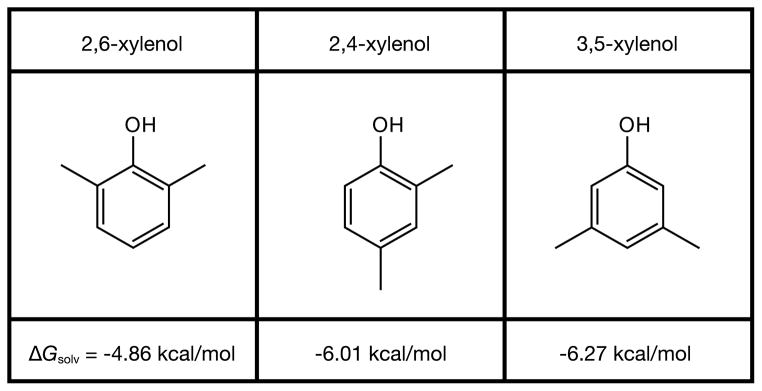
Experimental solvation free energies for a series of xylenol compounds determined from Henry’s Law constants [8]. Additivity does not hold. Because the chemical substituents are identical for all three, additivity would require identical solvation free energies

Another example of non-additivities is shown in Fig. 3. It shows that the solvation free energy of a hydroxybenzene molecule depends on the relative positions of the hydroxyl groups around the benzene ring. In this case, adding one hydroxyl group to a benzene ring contributes −5.7 kcal/mol to the free energy of transferring the hydroxybenzene molecule from air to water. Adding a second hydroxyl group contributes twice this amount of free energy, but only if the hydroxyl groups are maximally separated around the ring. If two hydroxyl groups are spatially close together, their contributions to ΔG_solv are less than would be predicted by additivity. If the hydroxyls are immediately adjacent and can form an intramolecular hydrogen bond with each other, then the total ΔG_solv for the molecule having two groups is essentially the same as a molecule with only a single hydroxyl group. In that case, adding a second hydroxyl group contributes nothing additional to the solvation free energy.

Fig. 3.

Non-additivities in a series of hydroxybenzenes calculated from Henry’s law constants [29, 42, 66]

Non-additivities can arise when the solvation shells of different substituents overlap with each other. Figure 4 shows that adding one nitrate group to an alkyl chain favors the transfer of butylnitrate from air to water by −3.8 kcal/mol, no matter where the nitrate group is located on the chain. However, adding a second nitrate group to the chain will double this free energy only if the two nitrate groups are sufficiently separated along the chain. If the two nitrate groups are close together in space, each nitrate group contributes less than would be predicted by additivity. The non-additivity arises from crowding and sharing of the solvation shells of the two nitrate groups. Water molecules in such shared solvation shells are often unable to freely solvate the nitrate groups as they would in either individual shell alone.

Fig. 4.

Experimental solvation free energies for the butylnitrate series calculated from Henry’s Law Coefficients [17, 29, 35]. An example of non-additivity. One nitrate group contributes −3.8 kcal/mol to ΔG_solv for transferring the butane chain from air to water. But, a second nitrate group contributes less than that if the nitrate groups are close together in space

The non-additivities described above are not negligible. Sometimes, these errors in solvation free energies are sufficiently large to render additivity-based models quantitatively useless. In order to develop more accurate methods for fast computational solvation modeling—for predicting solubilities, transfer, partitioning, binding affinities, and protein folding—it is helpful to look at the underlying causes of these errors.

2.2 The Structural Basis for Non-additivities of Solvation Free Energies

Water molecules in shared solvation shells behave differently than water molecules that are not shared; see Fig. 5. When component subgroups are distant from each other, their water shells are mostly independent of each other. But when solvation shells overlap, the water molecules that are shared can be in environments with unique constraints of hydrogen-bonding, sterics, and collective electrostatics that are not simple sums of the individual environments from the components. All-atom simulations in explicit-water can give insights into how water molecules behave in those cases.

Fig. 5.

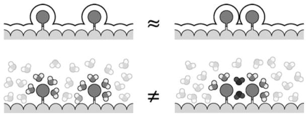
The origins of non-additivities in solvation free energies. (Top) Illustrating water-shell additivities. (Bottom) Illustrating that water molecules are particulate and can be constrained differently in shared environments than in unshared environments

2.2.1 Explaining the Xylenol and Dihydroxybenzene Series

Figure 6a shows the result of explicit-water simulations of the aqueous solvation of two different xylenols. In both cases, a single key water molecule accepts a hydrogen-bond from the hydroxyl group on the xylenol molecule. In (a), that key water molecule forms a strong hydrogen-bond; the OH · · · O angle is 180° and the average water dipole is directed along this axis. In (b), the same key water molecule is now obstructed by the neighboring methyl groups on the xylenol, preventing a good hydrogen-bond. This confinement of the hydroxyl group by the neighboring methyl groups decreases the solubility in water by 1.4 kcal/mol.

Fig. 6.

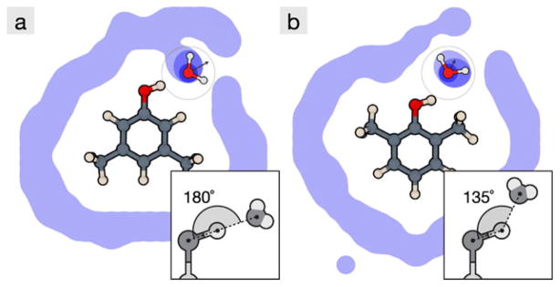
A slice of water density around: (a) 3,5-dimethylphenol and (b) 2,6-dimethylphenol, from explicit water simulations. A crucial structured water is observed in both cases, and the insets show details of the geometry. In (a), the structured water forms a strong hydrogen bond with the hydroxyl group on the xylenol, so it solvates more favorably than in (b), where the same hydrogen bond is impeded by the neighboring methyl groups. Color online

Even larger non-additivities arise in the dihydroxybenzene series. 1,2-dihydroxybenzene has nearly the same hydration free energy as phenol, even though the former has an extra –OH group (see Fig. 3). The explanation is that the two neighboring –OH groups in 1,2-dihydroxybenzene can form an intramolecular hydrogen-bond with each other, preventing favorable hydrogen bonding with water.

2.2.2 Ion-Ion Pairing Often Involves Shared Bridging Waters

Ion-ion interactions are common in chemistry and biology, for example salt bridges, contacts between charged amino acids, are often seen in protein structures. Such salt bridges are often separated by a bridging water molecule. Accounting for bridging waters in continuum electrostatics calculations has been shown to improve estimates of pairing energies [72].

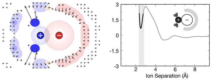
Figure 7 shows computer simulations of a potassium and fluoride ion approaching one another in water [14]. When the two ions are distant, their hydration shells are independent of each other and uniform relative to the ion-ion axis (Fig. 7a). But, as the ions get closer, the intervening water molecules become highly structured. The water molecules that are most highly structured are those that bridge between the two ions, but water molecules also become structured even around the backsides of the ions (Fig. 7c). Such structuring and sharing of water molecules lead to the several kcal/mol oscillations seen in the potential of mean force (PMF). First, as the ions approach each other, the ion-ion electrostatic attraction strengthens, accounting for the fact that the contact minimum (Fig. 7d) is the most stable state. The solvent-shared state of the two ions is further stabilized by the bridging water molecules, which have favorable electrostatic interactions with both ions (Fig. 7b). The transition state (Fig. 7c) is less stable because the bridging water is now partly squeezed out into a non-optimal orientation, and the remaining first-shell waters are then caged in an entropically unfavorable way that reduces the number of water molecules in this shell (resulting in depleted density on the backsides of the ions).

Fig. 7.

Water density maps for KF as a function of ion separation distance alongside a plot of the potential of mean force (in kcal/mol) between the ions. The separation distances highlight the (a) solvent-separated state, (b) the solvent-shared state, (c) the most unfavorable maximum, and (d) the contact state. The color indicates which ion the water density is closer to, blue for the cation and red for the anion, while the vectors indicate average direction and magnitude of water’s dipole moment in that region of space about the ions. Color online

The charges and sizes of the solute ions have a large effect on the structuring and energetics of intervening waters. The example above shows the situation for potassium fluoride, in which the cation and anion are about the same size. But, Fig. 8 shows that the situation is different for lithium iodide, where one ion is small (lithium) and the other is large. Unlike KF, the most stable state for LiI is separated by solvent. For LiI, the contact state is unfavorable because, in addition to direct hydration of lithium by water being more enthalpically favorable than a close ion-ion interaction, the hydrating water is structured in an entropically unfavorable way when the ions are in contact [14]. These size effects are key to explaining salt solubility products: small-small or large-large ion pairs are relatively insoluble in water, while small-large are more soluble [6].

Fig. 8.

Water density map about LiI in the contact state alongside a plot of the potential of mean force (in kcal/mol) between the ions. Water is tightly caged in this state, causing it to be entropically unfavorable. Color online

2.2.3 Solvation Free Energy Can Depend on Solute Curvature

Solvation free energy depends on the shape of the solute, such as its surface curvature, not just its surface area. Additivity methods often treat only the effects of surface area. Tanford noted that the interfacial tension between oil and water is about 75 cal/mol·Å², while the free energy of transfer of an oil molecule, say hexane, from oil to water is only 25 cal/mol·Å² [57, 65]. Subsequent work has shown that this is a consequence of the very tight curvature of a molecule relative to the very flat nature of a macroscopic interface, and incorporating the specifics of curvature can help correct for this difference [3, 57, 58].

2.2.4 Curvature Can Affect Pairing Interactions

Solute-solute PMFs also depend on the shapes of the solutes. For example all-atom explicit-solvent simulations have been performed in which a neutral surface contains a fixed charge embedded in it. The neutral surface was either concave (called a receptor), convex (called a bumper), or flat. A mobile ion of opposite charge was moved through a water solvent toward the fixed charge on the surface to calculate the PMF [5]. This calculation is like the ion-ion PMFs described above, except that now one of the ions is embedded in a surface of varying shape. A key finding is that the adjacent surface can strongly affect the ion-ion PMF. Figure 9 shows that the bumper surface (Figs. 9a and b) stabilizes the ion-ion solvent-separated state while the receptor surface stabilizes the ion-ion contact state (Figs. 9c and d). As noted above, much of this effect is due to water structuring. The bumper surface leads to strain in the water structuring by pushing caged waters closer to the ion-ion contact region (Fig. 9a), destabilizing the contact state. The receptor surface hinders hydrogen-bonding with bridging water, so the bridging waters are unable to compensate for the energy loss from separating the ions. So while water structuring can lead to several kcal/mol swings in the PMF, the shape of a nearby surface can alter the direction of these swings.

Fig. 9.

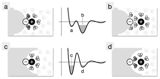
Illustration of the effect of surface curvature on the free energy of pairing for charges in solution. When the surface is changed from a convex bumper (a and b) to a concave receptor (c and d), the potential of mean force curves show an increasing favorability for the contact state over the solvent-separated state [5]

2.2.5 Not All Hydrocarbons Are the Same

The solvation properties are different for aromatic hydrocarbons than for aliphatic hydrocarbons. Figure 10 shows two homologous series: a series of alkane chains and a series of polyaromatic hydrocarbons of different lengths. For both, the non-polar components of the free energies of solvation are straight-line functions of their chain lengths. Both obey additivity relationships in terms of their constituent subgroups, methylene groups or benzene groups, respectively. However, the slopes of the two curves have opposite signs. For the non-polar components, longer alkanes are less soluble in water, while longer aromatic hydrocarbons are more soluble. These trends show that treating all hydrocarbons with a single γ in additive SA methods would not work; the non-polar component of ΔG_solv depends on the chemical differences among different types of hydrocarbons.

Fig. 10.

ΔG_np as a function of solvent-accessible surface area (SASA) for the linear alkane and linear polyaromatic hydrocarbon (PAH) series. The SASAs were computed from molecular dynamics simulations of uncharged molecules, and the ΔG_np for the alkanes come from experiment while the PAH values are from calculations in TIP3P water

2.2.6 Negative Charges Are More Soluble in Water than Positive Charges Are

It has long been known that a negative ion will be more soluble in water than a corresponding positive ion of the same charge magnitude and size [37]. This has been explored in detail by molecular simulations [54]. Implicit solvation models, such as GB or PB, do not intrinsically capture this property. This asymmetry can be explained by the physical structure of the water molecule. Water’s partially positive hydrogens are more localized and close to the water molecule’s surface while the average location of the negative oxygen charge is closer to the geometric center of the water molecule. In classical terms, the center of water’s dipole is offset relative to water’s center of mass. Water’s positive charge can come closer to a neighboring negative ion than water’s negative charge can come to a positive ion of the same size. Because implicit-solvent models don’t treat water molecules explicitly, this asymmetry effect is handled in PB and GB models by empirical adjustment of the effective radii of cations relative to anions.

The importance of this electrostatic asymmetry has been studied by Mobley et al. in computer simulations in TIP3P explicit solvent. Figure 11 shows the water-dipole asymmetry around two hexagonal-ring-shaped molecules [44], which we call bracelets. We consider two different bracelets, both of which are net neutral. One bracelet has a methylene sized ‘head’ bead with a charge of +1, and the other five beads have a charge of −0.2 each. The other molecule is identical, but with all the charge signs inverted. In implicit water, there should be no difference in the solvation free energy between the two bracelets (Δ ΔG_solv = 0). However, computer simulations in explicit TIP3P water show instead that Δ ΔG_solv of approximately 10 kcal/mol; with the - head-bracelet molecule more soluble than the + head bracelet [44].

Fig. 11.

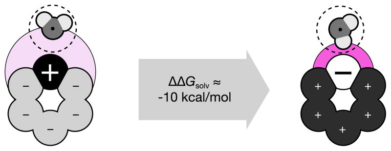
Illustration of the solvation asymmetry due to charge inversion for charge neutral small molecules. Water can position its positively charged hydrogens closer to negatively charged solute sites (right) than its negatively charged oxygen to positively charged solute atoms (left). This leads to an asymmetry in ΔG_solv in excess of 10 kcal/mol in some cases [44]. Color online

These calculations indicate that the charge-asymmetry effect can be substantial, even for solutes that are net neutral. While the molecules explored by Mobley et al. are fictitious, the underlying principles are not. Using fictitious molecules in computational experiments is useful for controlling variables to get insights into the origins of errors in more complex systems. This asymmetry is seen in some real molecules, such as the isostere pair of N,N-dimethylaniline and nitrobenzene, for which the solvation free energies, ΔG_solv, are about the same despite their drastically different dipole moments. Explicit solvent calculations are in better agreement with this experimental result than PB calculations [44].

3 Some Aspects of Non-additivity Are Handled by Implicit-Solvent Models

Explicit-solvent simulations are often accurate enough to reproduce the trends in solvation [9, 45, 46, 59–61]; however, explicit-solvent free energy calculations come with a significant computational cost. Implicit-solvent models can be used to determine free energies of solvation much more quickly [4, 7, 13, 55]. Recent developments in implicit-solvent models have been made to target some of the above problem cases.

Most implicit-solvent models separate the solvation free energy into non-polar and polar components. The non-polar term accounts for the cost of opening a cavity in the solvent to fit the solute, as well as the dispersion interactions with the surroundings, and the polar term accounts for transferring the solute’s charges and partial charges into water.

3.1 The Non-polar Term in Implicit Solvation

The most common approach for treating the non-polar aspect of solvation in implicit models is a γ A term, with the γ value usually taken from the surface area to solvation free energy relationship for the linear alkanes. This γA value approximates both the cavity formation and dispersion interaction parts in one expression. Having one γ handle all non-polar components assumes alkane chains are the best representation for a general solvent, and this can be problematic, as evidenced by Fig. 10. Gallicchio et al. have recently applied the idea of separating the system into sets of atom types and finding individual γ and curve intercept values for each that better reproduce this chemical specificity [22]. Also, separating the cavity and dispersion terms has allowed for more physical treatments of the parts of non-polar solvation [19–21, 40]. Other models have taken these more physical approaches further in an attempt to reduce the need for free parameters based on atom types [64, 67], model hydrophobic effects with the aid of information theory [31, 32], and develop variational approaches to more directly treat dispersion and curvature effects [11, 56].

3.2 The Polar Term in Implicit Solvation

The two primary implicit approaches for calculating the polar component are PB and GB. As having a good dielectric boundary is a key aspect in such calculations [30], most of the developments in GB, for example, have involved improved routes at determining the Born radii that define this boundary [25, 47, 49, 50]. Adjustment of this boundary nearer to, or further from, the solute is a useful route for incorporating effects seen in explicit-solvent, like the asymmetry upon charge inversion. Latimer et al. recommended such a route in 1939 when they published their study on ion solvation [37], and a recent study by Purisima and Sulea has used such an approach to treat the charge-asymmetry effect about neutral molecules in general continuum electrostatic calculations [53]. However, while adjustment of radii and the solute boundary can correct for a specific property, it can lead to deviations in other properties. For example, when Chorny et al. modulated the PB boundary to match the activation energy barrier for ion-pairing near curved surfaces, agreement of the relative stability of the paired and unpaired states with explicit solvent was lost [5].

Other approaches have also been developed. One is the Langevin Dipoles (LD) model [18, 52, 70], which goes beyond the continuum approximation by using a dipole lattice for the solvent representation. For capturing the chemical nature of the underlying solute, breaking up solutes into a fixed set of atom types and assigning specific solvation weights to each is a popular route. This approach is used by the simple solvation model from Eisenberg and McLachlan [12], the hydration shell model [36], and the effective energy function (EEF1) model [38].

4 The Semi-explicit Assembly (SEA) Approach to Solvation

We have recently developed a computational approach to aqueous solvation called Semi-Explicit Assembly (SEA). SEA treats the physics of surface solvation in a discrete way that resembles explicit models, but can estimate solvation free energies much more quickly, like implicit models. First, like implicit models, SEA separates the total solvation into two components, non-polar and polar.

4.1 Improving Non-polar Solvation Modeling Using SEA

Here is how non-polar solvation is treated in SEA [15]. We start by performing free energy calculations in explicit water of uncharged Lennard-Jones (LJ) spheres that have different sizes and well-depths. From these calculations, we generate lookup tables of ΔG_np and tables of the average distance (r_w) of the first-shell of water to each sphere (Fig. 12a). These tables are only generated once for any given solvent and state point.

Fig. 12.

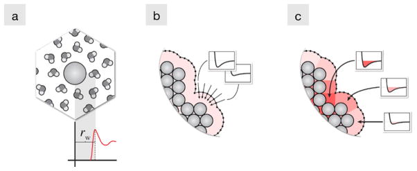
Illustration of the steps for constructing the non-polar SEA term. (a) Explicit solvent free energy calculations are performed on spheres to build tables of ΔG_np and water distance (r_w) values. (b) The solvent accessible surface is probed to determine the effective interaction potentials due to the environment. (c) The potentials are averaged and applied to the surface to incorporate non-polar environment effects. Color online

To determine the ΔG_np of a more complex solute, we assemble it from the known results from these LJ spheres. This involves first constructing a solvent accessible surface (SAS) from the distance tables, and probing the dispersion potential due to surrounding LJ atoms along normal vectors through points on this SAS (Fig. 12b). This results in a series of effective interaction potentials that describe the non-polar character of the interaction between the solute and the surrounding solvent. We then average these effective interaction potentials and extract new size and attraction parameters by fitting to an LJ potential (Fig. 12c). Thus, we compute the dispersion potential as if it were a local field, summed from all the solute atoms nearby. This means that we are replacing a γA quantity, which depends only on the nearest atom’s chemistry and surface area, with a free energy that also knows about neighboring chemistry and geometry. Finally, we apply these extracted LJ parameters to the surface atoms of the solute, and we sum up a total ΔG_np. This process retains the advantage of additivity, but eliminates the problems of an additivity that is too localized.

We have shown previously that the SEA approach improves upon some implicit methods of non-polar solvation. In a test of 504 small molecules, it was able to predict ΔG_np values that had only a 0.3 kcal/mol root mean squared error (RMSE) from detailed explicit solvent calculations [15], a 1 kcal/mol improvement over γA. Figure 13 illustrates the physical reason for the improvement: some hydrocarbons have different types and higher densities of LJ contributions at certain regions. Hence, alkynes (pentyne in the figure) have better solvation free energies than alkanes, because the triple-bonded hydrocarbon atoms are more attractive. For pyrene, SEA captures the increased attractiveness of the aromatic carbons (like for pentyne), but also the collective dispersion attraction of the face of the molecule over the edges.

Fig. 13.

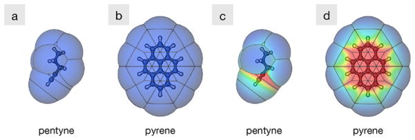
Maps of the attractive character of pentyne and pyrene reproduced using (a and b) a γA approach and (c and d) SEA. SEA captures the solvation attractiveness of the triple-bond structure in pentyne and the collective attraction of the aromatic carbons that are missed if one only uses a single γ term for the entire molecule. Color online

4.2 Improving Polar Solvation Modeling Using SEA

For solvating polar solutes, we treat the solvent distant from the solute surface as a continuum, as in implicit models. However, we treat the closer solvation shells more explicitly [16]. This again involves pre-simulations of LJ spheres in explicit water, only this time we also vary the solute charge. From each such simulation, we again collect r_w values, among other properties, but most importantly, we determine an average representation of a surface water molecule about this solute sphere. This is done by aligning all of the first-shell water molecules onto a common axis normal to the surface of the solute and binning the solvent atom locations to form density maps of the surface water charges. From these maps, we extract dipole moments that capture the first-shell polar response of these local water molecules.

To determine the polar aspect of the solvation free energy (ΔG_pol), we generate a solvent accessible dot surface about the solute of interest (Fig. 14a) and populate sites on this surface with the extracted dipole representations in accordance with the local electric field. The random placement procedure continues until all possible solvation sites are occupied or eliminated (Fig. 14b). ΔG_pol is accumulated as a Coulomb sum of all partial charges in the semi-explicit region (the spherical cavity in Fig. 14b). Because positional and orientational distributions of surface water molecules are factored into the dipole representations, this pairwise sum effectively approximates a free energy rather than simple potential energy. Outside this cavity, we use a reaction field to approximate distant electrostatic effects [48]. Finally, this random sampling process is iterated until ΔG_solv converges to a specified accuracy.

Fig. 14.

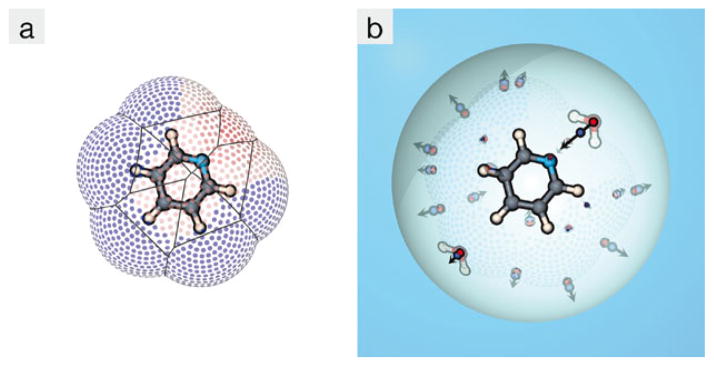
Illustration of SEA sampling process around pyridine. (a) A solvent-accessible dot surface is generated about the solute, and (b) semi-explicit dipoles are placed at sites on this dot surface according to the local electric field (indicated by the color of the surface dots) within a continuum dielectric cavity. Two of these dipoles are given water illustrations to highlight the direction the water dipoles point, and the magnitude of these dipoles indicate that the field is much stronger near the nitrogen that elsewhere around the pyridine. Color online

We have recently shown that SEA is able to quantitatively reproduce explicit-solvent ΔG_solv values to nearly 1k_BT accuracy over a large small molecule test set [16]. In comparisons to experimental ΔG_solv values, SEA was approximately 1k_BT lower RMSE than PB calculations, nearly the same as explicit-solvent calculations. SEA is more computationally efficient than either explicit solvent or PB free energy calculations; however, the advantage of SEA, in principle, is that it captures discrete water effects in the first shell, including physical details that are missing in purely continuum-solvent models.

5 SEA Captures Some of the Non-additivities in Solvation Free Energies

Here we compare how molecular simulations reproduce non-additivities in solvation free energies by considering the experimental non-additivity examples from the beginning of the text. We compare with experiment the following: TIP3P explicit solvent free energy calculations [34], PB with a traditional γA non-polar term [1], and SEA [15, 16]. Methods are as published elsewhere, [16, 45] with the exception that the SEA and PB results are the average of 100 solute conformations extracted from the TIP3P simulations (run using GROMACS 4.0.7) [2, 28]. All solutes used the general Amber Force Field (GAFF) [69]. AM1-BCC partial charges were set using ANTECHAMBER [33, 68]. To prevent PB from overly stabilizing hydroxyls (the hydrogen does not have Lennard-Jones parameters in GAFF), a generic LJ sphere (σ = 2.4 Å and ε = 0.02 kcal/mol) was applied to the hydrogen atom. This sphere is unnecessary in explicit and SEA calculations, and omitted in these cases.

For the xylenols shown in Fig. 2, there is a 1.4 kcal/mol Δ ΔG_solv from 2,6-dimethylphenol to 3,5-dimethylphenol (see Table 1). Explicit-solvent simulations and SEA capture most of this variation and show the correct trends, this despite the GAFF+AM1-BCC force field combination systematically under-predicting the solvation favorability of hydroxyl groups. Of more interest is the Δ ΔG_solv for PB, which is significantly smaller (0.3 kcal/mol) than that seen with explicit solvent and SEA. This is a case where the presence of discrete water appears to lead to more quantitative agreement with the non-additive behavior seen in experiment. This is understandable given Fig. 5, which shows that the non-additivity involves distortion of first-shell water hydrogen bonding.

Table 1.

ΔG_solv in kcal/mol for the xylenol series

Molecule	TIP3P	PBSA	SEA	Expt.a
2,6-xylenol	−4.18(3)	−5.12(3)	−3.84(5)	−4.86
2,4-xylenol	−4.51(5)	−5.53(3)	−4.62(8)	−6.01
3,5-xylenol	−5.38(3)	−5.45(3)	−4.93(5)	−6.27

^aReference [8]

Table 2 shows that explicit-solvent modeling captures the solvation trends well for the hy-droxybenzenes. It captures the shared-water effects as the substituents come close together on the benzene framework; see Fig. 15a. The figure shows the ΔG_solv benefit associated with the addition of each hydroxyl group. Deviations from a horizontal line indicate non-additivities. Explicit-solvent simulations capture about half of the experimentally observed non-additivity. This under-prediction is likely due the static partial charge nature of these calculations, and may improve with the inclusion of more detailed electrostatic interactions, such as polarization.

Table 2.

ΔG_solv in kcal/mol for the hydroxybenzene series

Molecule	TIP3P	PBSA	SEA	Expt.
benzene	−0.79(2)	−1.93(1)	−0.84(1)	−0.89a
phenol	−5.63(4)	−5.76(4)	−5.21(6)	−6.58a
1,2-dihydroxybenzene	−7.80(8)	−8.4(1)	−8.1(2)	−6.9b
1,3-dihydroxybenzene	−10.08(5)	−9.10(4)	−9.18(6)	−11c
1,4-dihydroxybenzene	−10.19(6)	−9.60(6)	−9.8(1)	−12b

^aReference [29],

^bRef. [42],

^cRef. [66]

Fig. 15.

Average solvation free energy gain per (a) hydroxyl group of the hydroxybenzene series and (b) nitrate group for the butylnitrate series seen in experiment and explicit solvent, PBSA [1], and SEA calculations [16]. The R-group in (b) represents a nitrate group, as in Fig. 4. Color online

SEA and PB both capture most of the non-additivity observed from the explicit-solvent simulations in this case. Their similar performance indicate that the loss in hydrogen-bonds to the hydroxyls can be fairly well approximated by a loss in solvent contact area to these hydrophilic groups upon formation of the intramolecular hydrogen bond.

The non-additivity in the butylnitrate series is more subtle than the other two series; it involves crowding of favorable hydration shells about the solute. Solvation is less favorable when the nitrate groups are close and more favorable when the groups are on opposite ends of the solute. Table 3 shows that explicit-solvent calculations faithfully reproduce this trend. Again, however, the magnitude of the solvation favorability of the functional group (a nitrate group this time) is systematically different from that seen in experiments. This over-favorability is likely due to the over-polarization of the nitro group from the ANTECHAMBER implementation of AM1-BCC approach. Alternative tools have shown less favorable solvation for nitro groups [45].

Table 3.

ΔG_solv in kcal/mol for the nitrate series

Molecule	TIP3P	PBSA	SEA	Expt.
butane	2.54(3)	1.02(1)	1.91(1)	2.17a
2-butylnitrate	−2.63(4)	−3.19(2)	−2.55(2)	−1.6b
1-butylnitrate	−2.85(3)	−3.05(2)	−2.57(3)	−1.8b
2,3-butanol dinitrate	−6.6(2)	−7.10(4)	−6.14(6)	−3.40c
1,2-butanol dinitrate	−6.60(4)	−7.20(5)	−5.98(7)	−3.72c
1,3-butanol dinitrate	−6.9(1)	−7.25(5)	−6.53(7)	−4.33c
1,4-butanol dinitrate	−7.28(7)	−7.35(4)	−7.21(6)	−4.93c

^aReference [29],

^bRef. [35],

^cRef. [17]

Aside from the experimental offset, Fig. 15b shows that TIP3P simulations are able to capture most of the experimental non-additivity. This non-additivity is also captured well by SEA, but missed by PB. Non-additivity due to hydration shell crowding is more complex than those due to strong intramolecular interactions insofar as it involves both significant polar and non-polar contributions.

6 Conclusions

We review computational modeling of the solvation of small solutes in water. Historically, two fast computational methods have been used to estimate free energies of solvation: (1) methods that sum the non-polar free energies of constituent atoms or subgroups, based on additivity relationships, and (2) implicit-solvent methods for treating the effects of solute charges. However, experiments and explicit solvent computer simulations show systematic deviations from additivities and from some of these continuum-electrostatic approximations. Explanations for those problems have emerged from computer simulations using explicit-water models. Some of these problems are: (1) Moieties that are close in space distort shared water molecules differently than single moieties do alone. (2) Additivities that are too local capture only effects of surface area (γA term), but not effects of solute shape and chemical structure, which can often be important. (3) Water’s electric dipole is offset from water’s center of mass, leading to asymmetries in how water solvates positive and negative charges. Some of these problems are being addressed in a new approach, called Semi-Explicit Assembly, that aims to capture more of the physics in explicit-solvent models, but with efficiencies approaching those of current implicit-solvent models. We see that it is able to physically model discrete first-shell water and reproduce experimentally observed non-additivities in solvation free energies nearly as well as detailed explicit-solvent calculations.

References

- 1.Baker NA, Sept D, Joseph S, Holst MJ, McCammon JA. Electrostatics of nanosystems: application to microtubules and the ribosome. Proc Natl Acad Sci USA. 2001;98(18):10037–10041. doi: 10.1073/pnas.181342398. [DOI] [PMC free article] [PubMed] [Google Scholar]
- 2.Berendsen HJC, van der Spoel D, van Drunen R. GROMACS: a message-passing parallel molecular dynamics implementation. Comput Phys Commun. 1995;91:43–56. [Google Scholar]
- 3.Chan HS, Dill KA. Solvation: effects of molecular size and shape. J Chem Phys. 1994;101(8):7007–7026. [Google Scholar]
- 4.Chen J, Brooks CL., III Implicit modeling of nonpolar solvation for simulating protein folding and conformational transitions. Phys Chem Chem Phys. 2008;10:471–481. doi: 10.1039/b714141f. [DOI] [PubMed] [Google Scholar]
- 5.Chorny I, Dill KA, Jacobson MP. Surfaces affect ion pairing. J Phys Chem B. 2005;109(50):24056–24060. doi: 10.1021/jp055043m. [DOI] [PubMed] [Google Scholar]
- 6.Collins KD. Charge density-dependent strength of hydration and biological structure. Biophys J. 1997;72 (1):65–76. doi: 10.1016/S0006-3495(97)78647-8. [DOI] [PMC free article] [PubMed] [Google Scholar]
- 7.Cramer CJ, Truhlar DG. Implicit solvation models: equilibria structure, spectra, and dynamics. Chem Rev. 1999;99(8):2161–2200. doi: 10.1021/cr960149m. [DOI] [PubMed] [Google Scholar]
- 8.Daubert T, Danner R. Physical and Thermodynamical Properties of Pure Chemicals: Data Compilation. Taylor & Francis; Washington: 1989. [Google Scholar]
- 9.Deng Y, Roux B. Hydration of amino acid side chains: nonpolar and electrostatic contributions calculated from staged molecular dynamics free energy simulations with explicit water molecules. J Phys Chem B. 2004;108(42):16567–16576. [Google Scholar]
- 10.Dill KA. Additivity principles in biochemistry. J Biol Chem. 1997;272(2):701–704. doi: 10.1074/jbc.272.2.701. [DOI] [PubMed] [Google Scholar]
- 11.Dzubiella J, Swanson JMJ, McCammon JA. Coupling hydrophobicity, dispersion, and electrostatics in continuum solvent models. Phys Rev Lett. 2006;96(8):087802. doi: 10.1103/PhysRevLett.96.087802. [DOI] [PubMed] [Google Scholar]
- 12.Eisenberg D, McLachlan AD. Solvation energy in protein folding and binding. Nature. 1986;319:199–203. doi: 10.1038/319199a0. [DOI] [PubMed] [Google Scholar]
- 13.Feig M, Brooks CL., III Recent advances in the development and application of implicit solvent models in biomolecule simulations. Curr Opin Struct Biol. 2004;14(2):217–224. doi: 10.1016/j.sbi.2004.03.009. [DOI] [PubMed] [Google Scholar]
- 14.Fennell CJ, Bizjak A, Vlachy V, Dill KA. Ion pairing in molecular simulations of aqueous alkali halide solutions. J Phys Chem B. 2009;113(19):6782–6791. doi: 10.1021/jp809782z. [DOI] [PMC free article] [PubMed] [Google Scholar]
- 15.Fennell CJ, Kehoe C, Dill KA. Oil/water transfer is partly driven by molecular shape, not just size. J Am Chem Soc. 2010;132(1):234–240. doi: 10.1021/ja906399e. [DOI] [PMC free article] [PubMed] [Google Scholar]
- 16.Fennell CJ, Kehoe CW, Dill KA. Modeling aqueous solvation with semi-explicit assembly. Proc Natl Acad Sci USA. 2011 doi: 10.1073/pnas.1017130108. [DOI] [PMC free article] [PubMed] [Google Scholar]
- 17.Fischer RG, Ballschmiter K. Prediction of the environmental distribution of alkyl dinitrates—chromatographic determination of vapor pressure p0, water solubility SH2O, gas-water partition coefficient kGW (Henry’s law constant) and octanol-water partition coefficient kOW. Fresenius J Anal Chem. 1998;360:769–776. [Google Scholar]
- 18.Florián J, Warshel A. Calculations of hydration entropies of hydrophobic, polar, and ionic solutes in the framework of the Langevin dipoles solvation model. J Phys Chem B. 1999;103(46):10282–10288. [Google Scholar]
- 19.Gallicchio E, Kubo MM, Levy RM. Enthalpy-entropy and cavity decomposition of alkane hydration free energies: numerical results and implications for theories of hydrophobic solvation. J Phys Chem B. 2000;104(26):6271–6285. [Google Scholar]
- 20.Gallicchio E, Levy RM. AGBNP: an analytic implicit solvent model suitable for molecular dynamics simulations and high-resolution modeling. J Comput Chem. 2004;25(4):479–499. doi: 10.1002/jcc.10400. [DOI] [PubMed] [Google Scholar]
- 21.Gallicchio E, Paris K, Levy RM. The AGBNP2 implicit solvation model. J Chem Theory Comput. 2009;5 (9):2544–2564. doi: 10.1021/ct900234u. [DOI] [PMC free article] [PubMed] [Google Scholar]
- 22.Gallicchio E, Zhang LY, Levy RM. The SGB/NP hydration free energy model based on the surface generalized Born solvent reaction field and novel nonpolar hydration free energy estimators. J Comput Chem. 2002;23(5):517–529. doi: 10.1002/jcc.10045. [DOI] [PubMed] [Google Scholar]
- 23.Gilson MK. Theory of electrostatic interactions in macromolecules. Curr Opin Struct Biol. 1995;5:216–223. doi: 10.1016/0959-440x(95)80079-4. [DOI] [PubMed] [Google Scholar]
- 24.Gilson MK, Honig B. Calculation of the total electrostatic energy of a macromolecular system: solvation energies, binding energies and conformational analysis. Proteins. 1988;4:7–18. doi: 10.1002/prot.340040104. [DOI] [PubMed] [Google Scholar]
- 25.Hawkins GD, Cramer CJ, Truhlar DG. Pairwise solute descreening of solute charges from a dielectric medium. Chem Phys Lett. 1995;246:122–129. [Google Scholar]
- 26.Hawkins GD, Cramer CJ, Truhlar DG. Parametrized models of aqueous free energies of solvation based on pairwise descreening of solute atomic charges from a dielectric medium. J Phys Chem. 1996;100(51):19824–19839. [Google Scholar]
- 27.Hermann RB. Theory of hydrophobic bonding. II The correlation of hydrocarbon solubility in water with solvent cavity surface area. J Phys Chem. 1972;76(19):2754–2759. [Google Scholar]
- 28.Hess B, Kutzner C, van der Spoel D, Lindahl E. GROMACS 4: algorithms for highly efficient, load-balanced, and scalable molecular simulation. J Chem Theory Comput. 2008;4(3):435–447. doi: 10.1021/ct700301q. [DOI] [PubMed] [Google Scholar]
- 29.Hine J, Mookerjee PK. The intrinsic hydrophilic character of organic compounds. Correlations in terms of structural contributions. J Org Chem. 1975;40:292–298. [Google Scholar]
- 30.Honig B, Nicholls A. Classical electrostatics in biology and chemistry. Science. 1995;268(5214):1144–1149. doi: 10.1126/science.7761829. [DOI] [PubMed] [Google Scholar]
- 31.Hummer G. Hydrophobic force field as a molecular alternative to surface-area models. J Am Chem Soc. 1999;121(26):6299–6305. [Google Scholar]
- 32.Hummer G, Garde S, García AE, Pohorille A, Pratt LR. An information theory model of hydrophobic interactions. Proc Natl Acad Sci USA. 1996;93:8951–8955. doi: 10.1073/pnas.93.17.8951. [DOI] [PMC free article] [PubMed] [Google Scholar]
- 33.Jakalian A, Bush BL, Jack DB, Bayly CI. Fast, efficient generation of high-quality atomic charges. AM1-BCC model: I Method. J Comput Chem. 2000;21(2):132–146. doi: 10.1002/jcc.10128. [DOI] [PubMed] [Google Scholar]
- 34.Jorgensen WL, Chandrasekhar J, Madura JD, Impey RW, Klein ML. Comparison of simple potential functions for simulating liquid water. J Chem Phys. 1983;79(2):926–935. [Google Scholar]
- 35.Kames J, Schurath U. Alkyl nitrates and bifunctional nitrates of atmospheric interest: Henry’s law constants and their temperature dependencies. J Atmos Chem. 1992;15(1):79–95. [Google Scholar]
- 36.Kang YK, Nemethy G, Scheraga HA. Free energies of hydration of solute molecules 1. Improvement of the hydration shell model by exact computations of overlap volumes. J Chem Phys. 1987;91:4105–4109. [Google Scholar]
- 37.Latimer WM, Pitzer KS, Slansky CM. The free energy of hydration of gaseous ions, and the absolute potential of the normal calomel electrode. J Chem Phys. 1939;7(2):108–111. [Google Scholar]
- 38.Lazaridis T, Karplus M. Effective energy function for proteins in solution. Proteins, Struct Funct Genet. 1999;35:133–152. doi: 10.1002/(sici)1097-0134(19990501)35:2<133::aid-prot1>3.0.co;2-n. [DOI] [PubMed] [Google Scholar]
- 39.Lee M, Salsbury FJ, Brooks CI. Novel generalized born methods. J Chem Phys. 2002;116(24):10606–10614. [Google Scholar]
- 40.Levy RM, Zhang LY, Gallicchio E, Felts AK. On the nonpolar hydration free energy of proteins: surface area and continuum solvent models for the solute-solvent interaction energy. J Am Chem Soc. 2003;125(31):9523–9530. doi: 10.1021/ja029833a. [DOI] [PubMed] [Google Scholar]
- 41.Luo R, David L, Gilson MK. Accelerated Poisson-Boltzmann calculations for static and dynamic systems. J Comput Chem. 2002;23(13):1244–1253. doi: 10.1002/jcc.10120. [DOI] [PubMed] [Google Scholar]
- 42.Mackay D, Shiu WY, Ma KC. Oxygen, Nitrogen, and Sulfur Containing Compounds. IV. Lewis Publishers; Boca Raton: 1995. Illustrated Handbook of Physical-Chemical Properties and Environmental Fate for Organic Chemicals. [Google Scholar]
- 43.Mark AE, van Gunsteren WF. Decomposition of the free energy of a system in terms of specific interactions: implications for theoretical and experimental studies. J Mol Biol. 1994;240:167–176. doi: 10.1006/jmbi.1994.1430. [DOI] [PubMed] [Google Scholar]
- 44.Mobley DL, Barber AE, II, Fennell CJ, Dill KA. Charge asymmetries in hydration of polar solutes. J Phys Chem B. 2008;112(8):2405–2414. doi: 10.1021/jp709958f. [DOI] [PMC free article] [PubMed] [Google Scholar]
- 45.Mobley DL, Bayly CI, Cooper MD, Shirts MR, Dill KA. Small molecule hydration free energies in explicit solvent: an extensive test of fixed-charge atomistic simulations. J Chem Theory Comput. 2009;5 (2):350–358. doi: 10.1021/ct800409d. [DOI] [PMC free article] [PubMed] [Google Scholar]
- 46.Mobley DL, Dumont E, Chodera JD, Dill KA. Comparison of charge models for fixed-charge force fields: small-molecule hydration free energies in explicit solvent. J Phys Chem B. 2007;111(9):2242–2254. doi: 10.1021/jp0667442. [DOI] [PubMed] [Google Scholar]
- 47.Mongan J, Simmerling C, McCammon JA, Case DA, Onufriev A. Generalized born model with a simple, robust molecular volume correction. J Chem Theory Comput. 2006;3(1):156–169. doi: 10.1021/ct600085e. [DOI] [PMC free article] [PubMed] [Google Scholar]
- 48.Onsager L. Electric moments of molecules in liquids. J Am Chem Soc. 1936;58(8):1486–1493. [Google Scholar]
- 49.Onufriev A, Bashford D, Case D. Modification of the generalized born model suitable for macromolecules. J Phys Chem B. 2000;104(15):3712–3720. [Google Scholar]
- 50.Onufriev A, Case DA, Bashford D. Effective born radii in the generalized born approximation: the importance of being perfect. J Comput Chem. 2002;23(14):1297–1304. doi: 10.1002/jcc.10126. [DOI] [PubMed] [Google Scholar]
- 51.Ooi T, Oobatake M, Nemethy G, Scheraga HA. Accessible surface areas as a measure of the thermodynamic parameters of hydration of peptides. Proc Natl Acad Sci USA. 1987;84:3086–3090. doi: 10.1073/pnas.84.10.3086. [DOI] [PMC free article] [PubMed] [Google Scholar]
- 52.Papazyan A, Warshel A. Effect of solvent discreteness on solvation. J Phys Chem B. 1998;102(27):5348–5357. [Google Scholar]
- 53.Purisima EO, Sulea T. Restoring charge asymmetry in continuum electrostatics calculations of hydration free energies. J Phys Chem B. 2009;113(24):8206–8209. doi: 10.1021/jp9020799. [DOI] [PubMed] [Google Scholar]
- 54.Rajamani S, Ghosh T, Garde S. Size dependent ion hydration, its asymmetry, and convergence to macroscopic behavior. J Chem Phys. 2004;120(9):4457–4466. doi: 10.1063/1.1644536. [DOI] [PubMed] [Google Scholar]
- 55.Roux R, Simonson T. Implicit solvent models. Biophys Chem. 1999;78:1–20. doi: 10.1016/s0301-4622(98)00226-9. [DOI] [PubMed] [Google Scholar]
- 56.Setny P, Wang Z, Cheng LT, Li B, McCammon JA, Dzubiella J. Dewetting-controlled binding of ligands to hydrophobic pockets. Phys Rev Lett. 2009;103(18):187801. doi: 10.1103/PhysRevLett.103.187801. [DOI] [PMC free article] [PubMed] [Google Scholar]
- 57.Sharp K, Nicholls A, Fine R, Honig B. Reconciling the magnitude of the microscopic and macroscopic hydrophobic effects. Science. 1991;252:106–109. doi: 10.1126/science.2011744. [DOI] [PubMed] [Google Scholar]
- 58.Sharp KA, Nicholls A, Friedman R, Honig B. Extracting hydrophobic free energies from experimental data: relationship to protein folding and theoretical models. Biochem. 1991;30(40):9686–9697. doi: 10.1021/bi00104a017. [DOI] [PubMed] [Google Scholar]
- 59.Shirts MR, Pande VS. Solvation free energies of amino acid side chain analogs for common molecular mechanics water models. J Chem Phys. 2005;122(13):134508. doi: 10.1063/1.1877132. [DOI] [PubMed] [Google Scholar]
- 60.Shirts MR, Pitera JW, Swope WC, Pande VS. Extremely precise free energy calculations of amino acid side chain analogs: comparison of common molecular mechanics force fields for proteins. J Chem Phys. 2003;119(11):5740–5761. [Google Scholar]
- 61.Shivakumar D, Williams J, Wu Y, Damm W, Shelley J, Sherman W. Prediction of absolute solvation free energies using molecular dynamics free energy perturbation and the OPLS force field. J Chem Theory Comput. 2010;6(5):1509–1519. doi: 10.1021/ct900587b. [DOI] [PubMed] [Google Scholar]
- 62.Sitkoff D, Sharp KA, Honig B. Accurate calculation of hydration free energies using macroscopic solvent models. J Phys Chem. 1994;98(7):1978–1988. [Google Scholar]
- 63.Still WC, Tempczyk A, Hawley RC, Hendrickson T. Semianalytical treatment of solvation for molecular mechanics and dynamics. J Am Chem Soc. 1990;112(16):6127–6129. [Google Scholar]
- 64.Tan C, Tan YH, Luo R. Implicit nonpolar solvent models. J Phys Chem B. 2007;111:12263–12274. doi: 10.1021/jp073399n. [DOI] [PubMed] [Google Scholar]
- 65.Tanford C. Interfacial free energy and the hydrophobic effect. Proc Natl Acad Sci USA. 1979;76(9):4175–4176. doi: 10.1073/pnas.76.9.4175. [DOI] [PMC free article] [PubMed] [Google Scholar]
- 66.USEPA. Tech Rep EPA-68-03-002. USEPA; Cincinnati, OH, USA: 1982. Air and steam stripping of toxic pollutants. [Google Scholar]
- 67.Wagoner JA, Baker NA. Assessing implicit models for nonpolar mean solvation forces: the importance of dispersion and volume terms. Proc Natl Acad Sci USA. 2006;103(22):8331–8336. doi: 10.1073/pnas.0600118103. [DOI] [PMC free article] [PubMed] [Google Scholar]
- 68.Wang J, Wang W, Kollman PA, Case DA. Automatic atom type and bond type perception in molecular mechanical calculations. J Mol Graph Model. 2006;25:247–260. doi: 10.1016/j.jmgm.2005.12.005. [DOI] [PubMed] [Google Scholar]
- 69.Wang J, Wolf RM, Caldwell JW, Kollman PA, Case DA. Development and testing of a general amber force field. J Comput Chem. 2004;25(9):1157–1174. doi: 10.1002/jcc.20035. [DOI] [PubMed] [Google Scholar]
- 70.Warshel A, Russell ST. Calculations of electrostatic interactions in biological systems and in solutions. Q Rev Biophys. 1984;17:283–422. doi: 10.1017/s0033583500005333. [DOI] [PubMed] [Google Scholar]
- 71.Yaws CL, Yang HC. Thermodynamic and Physical Property Data. Gulf Publishing Company; Houston: 1992. Henry’s law constant for compound in water; pp. 181–206. [Google Scholar]
- 72.Yu Z, Jacobson MP, Josovitz J, Rapp CS, Friesner RA. First-shell solvation of ion pairs: correction of systematic errors in implicit solvent models. J Phys Chem B. 2004;108(21):6643–6654. [Google Scholar]