Monitoring Protein Interactions in Living Cells with Fluorescence Lifetime Imaging Microscopy

Abstract

Fluorescence lifetime imaging microscopy (FLIM) is now routinely used for dynamic measurements of signaling events inside single living cells, such as monitoring changes in intracellular ions and detecting protein–protein interactions. Here, we describe the digital frequency domain FLIM data acquisition and analysis. We describe the methods necessary to calibrate the FLIM system and demonstrate how they are used to measure the quenched donor fluorescence lifetime that results from Förster Resonance Energy Transfer (FRET). We show how the “FRET-standard” fusion proteins are used to validate the FLIM system for FRET measurements. We then show how FLIM–FRET can be used to detect the dimerization of the basic leucine zipper (B Zip) domain of the transcription factor CCAAT/enhancer binding protein α in the nuclei of living mouse pituitary cells. Importantly, the factors required for the accurate determination and reproducibility of lifetime measurements are described in detail.

1. Introduction

The development of the many different genetically encoded fluorescent proteins (FPs), which now span the full visible spectrum, has sparked a revolution in optical imaging in biomedical research (Day and Davidson, 2009). These new FPs have expanded the repertoire of imaging applications from multi-color imaging of protein co-localization and behavior inside living cells to the detection of changes in intracellular activities, such as pH or ion concentration. However, it is the use of the genetically encoded FPs for Förster Resonance Energy Transfer (FRET) microscopy in living cells that has generated the most interest in these probes (Aye-Han et al., 2009; Giepmans et al., 2006; Piston and Kremers, 2007; Sun et al., 2011; Vogel et al., 2006).

FRET is the process by which energy absorbed by one fluorophore (the “donor”) is transferred directly to another nearby molecule (the “acceptor”) through a nonradiative pathway. This process depletes the excited-state energy of the donor molecule, quenching its fluorescence emission while causing increased (sensitized) emission from the acceptor. The quenching of the donor as well as the sensitized acceptor emission can be used to quantify energy transfer. Since the distance over which efficient energy transfer can occur is limited to less than 100 Å, FRET can be used to monitor protein–protein interactions inside living cells, tissues, and organisms (Miyawaki, 2011; Tsien, 2005; Yasuda, 2006; Zhang et al., 2002). There are many different methods used to measure FRET, each with distinct advantages and disadvantages, and these have been reviewed elsewhere (Jares-Erijman and Jovin, 2003; Periasamy and Day, 2005).

The most accurate methods for detecting FRET are the approaches that measure the change in the donor fluorescence lifetime that results from the quenching by the acceptor (Periasamy and Clegg, 2010). The fluorescence lifetime is the average time that a molecule spends in the excited state before returning to the ground state, which is usually accompanied by the emission of a photon. The fluorescence lifetime is an intrinsic property of each fluorophore, and most probes used in biological studies have lifetimes ranging between 1 to about 10 ns. The fluorescence lifetime of the fluorophore also carries information about events in the local microenvironment that can affect its photophysical behavior. Because energy transfer is a quenching process affecting the excited state of the donor fluorophore, the donor fluorescence lifetime is shortened by FRET.

Fluorescence lifetime imaging microscopy (FLIM) maps the spatial distribution of probe lifetimes inside living cells and can accurately measure the shorter donor lifetimes that result from FRET (Periasamy and Clegg, 2010; Sun et al., 2010, 2011; Wouters and Bastiaens, 1999; Yasuda, 2006). Here, we describe in detail the procedures that are necessary to use the frequency domain (FD) FLIM method to measure FRET, allowing us to monitor protein–protein interactions inside living cells. The basic calibration procedures necessary for accurate lifetime determinations are described. We demonstrate the measurement of FRET using protein standards designed to validate microscope systems for the detection of FRET (Koushik et al., 2006). We then use digital FD FLIM to characterize the dimerization of the transcription factor CAATT/enhancer binding protein α (C/EBPα) in regions of centromeric heterochromatin in the living cell nucleus. The methodology described here can be adapted for other commercial FLIM systems.

1.1. Overview of FRET microscopy

FRET involves the direct transfer of excited-state energy from a donor fluorophore to nearby acceptor molecules through near-field electromagnetic dipole interactions. There are three basic requirements for the efficient transfer of energy to the acceptor (Forster, 1965; Lakowicz, 2006; Stryer, 1978). First, because energy transfer involves electromagnetic dipolar interactions between the excited-state donor and the acceptor fluorophores, the efficiency of energy transfer (E_FRET) varies as the inverse of the sixth power of the distance (r) that separates the fluorophores. This sixth power dependence is described by the Förster equation (19.1):

$$E_{\text{FRET}}=\frac{R_0^6}{R_0^6+r^6}$$ (19.1)

where R₀ is the Förster distance at which the efficiency of energy transfer is 50%. The relationship of E_FRET to the distance separating the fluorophores is illustrated in Fig. 19.1A. Because E_FRET varies as the inverse of the sixth power of the separation distance between the fluorophores, the efficiency of energy transfer falls off sharply over the range of 0.5 R₀ to 1.5 R₀ (shaded area, Fig. 19.1A). This is why energy transfer between the FP-labeled proteins is limited to distances of less than approximately 100 Å.

Figure 19.1.

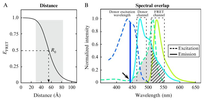
The distance dependence (A) and the spectral overlap (B) requirements for efficient FRET. (A) The efficiency of energy transfer, E_FRET, was determined using Eq. (19.1), and is plotted as a function of the separation distance in Å. The shaded region illustrates the range of 0.5 R₀ to 1.5 R₀ over which FRET can be accurately measured. (B) The excitation and emission spectra for the CFP (donor) and YFP (acceptor) FRET pair are shown, with the shaded region indicating the spectral overlap between the donor emission and acceptor excitation. The dashed boxes indicate the donor (480/40 nm) and FRET (530/43 nm) detection channels. The arrow indicates the direct acceptor excitation at the donor excitation wavelength, and the hatching shows donor SBT into the FRET channel.

The second requirement for efficient transfer of energy is the favorable alignment of the electromagnetic dipoles of the donor emission and acceptor absorption. The angular dependence of the donor and acceptor dipolar interaction is described by the orientation factor, κ². Depending on the relative orientation of the donor and acceptor, the value for κ² can range from 0 to 4 (Gryczynski et al., 2005). It is difficult, however, to determine κ² in most experimental systems. Fortunately, for many biological applications, where proteins labeled with the donor and acceptor fluorophores freely diffuse within cellular compartments and adopt a variety of conformations, the orientations of the FP tags randomize over the time scales of the measurements. Under these conditions, κ² is often assumed to be 2/3, which reflects the random orientations of the probes. However, if the donor and acceptor adopt unique orientations and are immobile on the time scale of FRET, then 2/3 will not accurately describe the dipolar orientation. Therefore, caution is necessary when assigning precise separation distances based on FRET measurements. The final requirement for FRET is that the fluorophores share a strong overlap between the donor emission spectrum and the absorption spectrum of the acceptor (see Fig. 19.1B). In this regard, it is desirable to select a donor fluorophore with a high quantum yield that shares significant (>30%) spectral overlap with the acceptor. The quantum yield of the acceptor is not important when the donor fluorescence lifetime is used to measure FRET, but it is critical that the acceptor has a high extinction coefficient. When these basic requirements for energy transfer are met, the quantification of FRET by microscopy can provide Angstrom-scale measurements of the spatial relationship between the fluorophore-labeling proteins inside living cells.

1.2. The FPs and FRET microscopy

The cloning of Aequorea green FP and the subsequent engineering to fine-tune its spectral characteristics yielded many different FPs with fluorescence emissions ranging from the blue to the yellow regions of the visible spectrum (Shaner et al. 2005; Tsien 1998). Currently, the cyan (CFP) and yellow (YFP) FPs are the most widely used for FRET-based imaging studies because of their significant spectral overlap (shaded area, Fig. 19.1B). The monomeric (m) mCerulean CFPs (Rizzo et al., 2004) used in combination with either the mVenus (Nagai et al., 2002) or mCitrine (Griesbeck et al., 2001) YFP are among the most popular FRET pairings. When energy is transferred from mCerulean to mVenus, the mCerulean emission signal detected in the donor channel is quenched, and there is increased (sensitized) emission from the acceptor, which is detected in the FRET channel (Fig. 19.1B). However, a consequence of the strong spectral overlap, which is required for FRET, is significant background fluorescence (called spectral bleed through, SBT) that is also detected in the FRET channel. The SBT results from the direct excitation of the acceptor by the donor excitation wavelengths (arrow, Fig. 19.1B) and the donor emission signal that bleeds into the FRET detection channel (hatching, Fig. 19.1B). Therefore, the accurate measurement of FRET by detecting sensitized emission signals requires correction methods that define and remove these different SBT components (Periasamy and Day, 2005). Significantly, the accuracy of these SBT correction methods is degraded as the spectral overlap between the FPs is increased to the point where the SBT components overwhelm the FRET signal (Berney and Danuser, 2003).

1.3. Overview of FLIM

The alternative to the SBT correction methods is to measure the effect of FRET on the donor fluorophore. Importantly, because the SBT background is detected in the acceptor emission (FRET) channel (see Fig. 19.1B), these artifacts can be avoided when making measurements in the donor channel. Since the transfer of energy quenches the emission from donors participating in FRET, the fluorescence lifetime of that donor population becomes shorter. Therefore, measuring the change in the donor fluorescence lifetime in the presence of the acceptor is the most direct method for monitoring FRET, and this is what FLIM does. FLIM is particularly useful for biological applications, since the donor fluorescence lifetime is a time measurement that is not affected by variations in the probe concentration, excitation intensity, and other factors that can limit intensity-based measurements.

The first measurements of the nanosecond decay of fluorescence using optical microscopy were made in 1959 (Venetta, 1959). The FLIM methodologies have evolved significantly in recent years and now encompass biological, biomedical, and clinical research applications (Periasamy and Clegg, 2010). The FLIM techniques are broadly subdivided into the time domain (TD) and the FD methods. The physics that underlies these two different methods is identical, only the analysis of the measurements differs (Clegg, 2010). The TD method uses a pulsed-laser source to excite the specimen. For probes with nanosecond lifetimes, femtosecond to picosecond pulse durations are used. The laser is synchronized to high-speed detectors that can record the arrival time of a single photon relative to the excitation pulse. The photons are accumulated at different time bins relative to the excitation pulse to build a histogram, which is analyzed to determine the fluorescence decay profile, providing an estimate of the fluorescence lifetime. In contrast, the FD method uses a light source modulated at high radio frequencies to excite a fluorophore and then measures the modulation and phase of the emission signals. The fundamental modulation frequency is chosen depending on the lifetime of the fluorophore and is usually between 10 and 100 MHz for the measurement of nanosecond decays. The emission signal is then analyzed for changes in phase and amplitude relative to the excitation source to extract the fluorescence lifetime of the fluorophore.

2. FD FLIM Measurements

The FD FLIM system described in this paper employs the technique called FastFLIM (Colyer et al., 2008), which measures the phase delays and modulation ratios at multiple frequencies simultaneously. Because of the finite lifetime of the excited state, there is a phase delay (Φ) and a change in the modulation (M) of the emission relative to the excitation waveform (Fig. 19.2). The lifetime of the fluorophores can be directly determined by measuring either the phase delays (the phase lifetime τ_Φ, Eq. 19.2) or the modulation ratio (the modulation lifetime τ_M, Eq. 19.3) at different modulation frequencies (ω).

Figure 19.2.

Frequency-domain (FD) FLIM setup. The excitation source for the FD FLIM system in this study is a 448-nm diode laser that is directly modulated by the ISS FastFLIM module at the fundamental frequency of 20 MHz. The modulated laser is coupled to the ISS scanning system that is attached to an Olympus IX71 microscope. The emission signals from the specimen travel through the scanning system (de-scanned detection) and are then routed by a beam splitter through the donor and acceptor emission channel filters to two identical APD detectors. The phase delays (Φ) and modulation ratios of the emission relative to the excitation are measured at up to seven modulation frequencies (ω = 20–140 MHz) for each XY raster scanning location. The basic principle of the FD FLIM method is illustrated, showing the phase delay (Φ) and modulation ratio (M = AC/DC) of the emission (Em) relative to the excitation (Ex) that are used to estimate the fluorescence lifetime.

$${\tau }_{\mathit{\Phi }}=\frac{tan\mathit{\Phi }}{\omega }$$ (19.2)

$${\tau }_{\mathrm{M}}=\sqrt{\frac{1-M^2}{(M\omega )}}$$ (19.3)

If the fluorescence decay from the fluorophores is best fit to a single exponential, then τ_Φ and τ_M will be the same at all ω. Conversely, if the decay is best fit by a multi-exponential, then τ_Φ < τ_M and their values will depend on the ω. Therefore, the FD FLIM method provides immediate information regarding lifetime heterogeneity within a system.

2.1. The analysis of FD FLIM measurements

The measurements from the FD FLIM method are commonly analyzed using the polar plot (also called a phasor plot) method. This method was originally developed as a way to analyze transient responses to repetitive perturbations, such as dielectric relaxation experiments, and can be applied to any system with frequency characteristics (Cole and Cole, 1941; Redford and Clegg, 2005). The polar plot directly displays the modulation fraction and the phase of the emission signal in every pixel in a FLIM image, allowing determination of the lifetime. The frequency characteristics at each image pixel are displayed with the coordinates x = M(ω) × cos Φ(ω) and y = M(ω) × sin Φ(ω). The relationship x² + y² = x defines a “universal” semicircle with a radius of 0.5 that is centered at {0.5, 0}. This semicircle describes the lifetime trajectory for any single lifetime component, with longer lifetimes to the left (0, 0 is infinite lifetime) and shorter lifetimes to right (Redford and Clegg, 2005). Most important, the polar plot does not require a fitting model to determine fluorescence lifetime distributions, but rather expresses the overall decay in each pixel in terms of the polar coordinates on the universal semicircle. A population of fluorophores that has only one lifetime component will result in a distribution of points that fall directly on the semicircle. In contrast, a population of fluorophores with multiple lifetime components will have a distribution of points that fall inside the semicircle.

2.2. The calibration of a FLIM system

Before imaging biological samples, it is necessary to calibrate the FLIM system using a fluorescence lifetime standard. The fluorescence lifetime for many fluorophores has been established under standard conditions (an online source is available at: http://www.iss.com/resources/reference/data_tables/LifetimeDataFluorophores.html), and any of these probes can be used for calibration of the FLIM system. Since the fluorescence lifetime of a fluorophore is sensitive to its environment, it is critical to prepare the standards according to the conditions specified in the literature, including the solvent and the pH. It is also important to choose a standard fluorophore with excitation, emission, and fluorescence lifetime properties that are similar to those of the fluorophore used in the biological samples. For example, the dye Coumarin 6 dissolved in ethanol (peak excitation and emission of 460 and 505 nm, respectively), with a reference lifetime of ~2.5 ns, is often used as the calibration standard for the CFPs. It is important to note that if the excitation wavelength is changed, it is necessary to recalibrate with an appropriate lifetime standard.

2.2.1. Required materials

2.2.1.1. Device and materials for FLIM measurements

Figure 19.2 shows the basic diagram of the digital FD FLIM system used here. The ISS ALBA FastFLIM system (ISS Inc., Champaign, IL) is coupled to an Olympus IX71 microscope equipped with a 60×/1.2 NA water-immersion objective lens. A Pathology Devices (Pathology Devices, Inc., Exton, PA) stage top environmental control system is used to maintain temperature at 36° C and CO₂ at 5%. A 5 mW, 448-nm diode laser is modulated by the FastFLIM module of the ALBA system at the fundamental frequency of 20 MHz with up to seven sinusoidal harmonics. The modulated laser is coupled to the ALBA scanning system, which is controlled by ISS VistaVision software (http://www.iss.com/microscopy/software/vistavision.html). The fluorescence signals emitted from the specimen are routed by a 495 nm long-pass beam splitter through the 530/43 nm (channel 1, acceptor emission) and the 480/40 nm (channel 2, donor emission) band-pass emission filters. The pinholes for each channel are set at 50 micrometer, and the signals are then detected using two identical avalanche photodiodes (APDs). The phase delays and modulation ratios of the emission relative to the excitation are measured at six modulation frequencies (20, 40, 60, 80, 100, 120 MHz) for each pixel of an image.

2.2.1.2. Additional materials

• Coumarin 6 (Sigma-Aldrich Inc., cat. # 546283)

• HPTS (8-Hydroxypyrene-1,3,6-trisulfonic acid, trisodium salt from AnaSpec Inc., cat. # 84610)

• Chambered cover glass (4 or 8 well; Thermo Scientific, cat. # 155382, 155409).

2.2.2. Calibration and validation

The calibration of the system with the Coumarin 6 dye provides the software with the reference standard that will be used to estimate the lifetime values from the experimental data. It is essential that the calibration is done before each experiment, and it is prudent to repeat the calibration several times during the experiment. Additionally, we use a second reference standard to check that the system is accurately reporting the fluorescence lifetime of a known sample. Here, we use HPTS dissolved in phosphate buffer (PB) pH 7.8 (peak excitation and emission at 454 and 511 nm, respectively), which has an expected lifetime of 5.3 ns.

The measurement of the fluorescence lifetimes for these two different probes is illustrated in Fig. 19.3. Following calibration of the system, we used the FD FLIM method to determine the fluorescence lifetime of Coumarin 6 in ethanol. A 256 × 256 pixel FLIM image was obtained from a chambered cover glass containing 50 μM Coumarin 6 in ethanol. Frame averaging is used to accumulate approximately 100 counts per pixel, and the distribution of the lifetimes for all the pixels in the image (a total of 65,536 pixels) is represented on the polar plot, allowing determination of an average lifetime of 2.5 ns (Fig. 19.3A). The distribution falls directly on the semicircle, indicating a single lifetime component for Coumarin 6. To verify that the system is accurately calibrated, measurements are then made of a second dye solution containing 10 mM HPTS dissolved in PB. The polar plot for the HPTS sample, shown in Fig. 19.3B, clearly demonstrates that the position of its lifetime distribution is shifted to the left along semicircle relative to Coumarin 6 (compare Fig. 19.3A and B). Again, the distribution falls directly on the semicircle and indicates a single lifetime component of 5.3 ns for HPTS.

Figure 19.3.

The polar plot analysis of the fluorescence lifetime of (A) Coumarin 6 in ethanol and (B) HPTS in PB, pH 7.8. The polar plot analysis was made using the first harmonic (20 MHz). (A) For Coumarin 6, the frequency characteristics for each pixel in the 256 × 256 image (65,536 points) are displayed on the polar plot with the coordinates x = M(ω) × cos Φ(ω), and y = M(ω) × sin Φ(ω). The vector length is determined from the modulation (M), and the phase delay (Φ) determines the angle. The centroid of the distribution falls on the universal semicircle, representing a single exponential lifetime of 2.5 ns. (B) For HPTS, each pixel in the 256 × 256 image is displayed on the polar plot, illustrating how the distribution for the longer lifetime probe is shifted to the left along the semicircle. The centroid of the distribution falls on the semicircle, indicating a single exponential lifetime of 5.3 ns.

2.3. Testing the FLIM system using “FRET-standard” proteins

Before making FLIM measurements from biological samples expressing FP-labeled proteins of interest that have not been characterized in FRET-based assays, it is advisable to test the system (both the cellular model and the microscope system) using “FRET-standard” proteins. The Vogel laboratory (Koushik et al., 2006; Thaler et al., 2005) created genetic constructs that encoded mCerulean directly coupled to mVenus through protein linkers of different lengths. For example, they generated a genetic construct that encoded mCerulean separated from mVenus by a five amino acid linker (Cerulean-5AA-Venus), producing a fusion protein with consistently high FRET efficiency. Since the fluorescence lifetime is very sensitive to the probe environment, an identical genetic construct that encodes Cerulean linked to a chromophore mutant of Venus, called Amber, was also generated (Koushik et al., 2006). Amber is a non-fluorescent form of Venus where the chromophore tyrosine was changed to cysteine, producing a protein that folds correctly, but does not act as a FRET acceptor. The Cerulean-5AA-Amber protein recapitulates the local environment of the Cerulean donor fluorophore without the quenching that results from energy transfer.

The Vogel laboratory also made genetic constructs with a larger linkers. For example, a linker that encoded the 229-amino acid tumor necrosis factor receptor-associated factor (TRAF) domain was inserted between the mCerulean and mVenus proteins (Cerulean-TRAF-Venus). This produced a fusion protein with low FRET efficiency. They then used three different techniques to measure FRET in cells that expressed the “FRET-standard” fusion proteins. For each of the fusion proteins tested, there was consensus in the results obtained by the different FRET methods, demonstrating that these genetic constructs could serve as FRET standards (Thaler et al., 2005). Most important, these genetic constructs have been freely distributed to many other laboratories, where they are routinely used to verify and evaluate FRET measurements obtained in different experimental systems.

2.3.1. Transfection of cells by electroporation

The mouse pituitary GHFT1 cells (Lew et al., 1993) used in our laboratory are efficiently transfected by electroporation. We established the following conditions by transfecting the cells with a plasmid containing the cytomegalovirus promoter driving the luciferase reporter gene (Promega, Madison, WI) using a range of different electroporation voltages. The highest level of luciferase protein expression in the GHFT1 cells was achieved at 200 V.

2.3.2. Required materials

2.3.2.1. Device and materials for electroporation

There are several commercially available systems for gene transfer by electroporation. We use the BTX ECM 830 device (Harvard Apparatus, Holliston, MA)

• Mouse pituitary GHFT1 cells (Lew et al., 1993) are maintained as monolayer cultures in Dulbecco’s modified Eagle’s medium (DMEM) containing 10% newborn calf serum (NBCS) at 37 °C in a 5% CO₂ incubator

• 0.05% Trypsin/0.53 mM ethylenediaminetetraacetic acid (EDTA) (Fisher Scientific Inc., cat. # MT25-051-Cl)

• 2-mm Gap electroporation cuvettes (BTX, cat. # 45-0125)

• Chambered cover glass (2 well; Thermo Scientific, cat. # 155379)

• Dulbecco’s phosphate-buffered saline (PBS)—calcium and magnesium free (Fisher, Cellgro, cat. # 21-031-CV)

• BioBrene (Applied Biosystems Inc., cat. #400385)

• Imaging media: Phenol red-free F12:DMEM (1:1) containing 10% NBCS (Sigma, cat. # D2906-10x1L). Since phenol red may cause background fluorescence signals, it is important to use a phenol red-free medium during imaging

• Cerulean-5AA-Amber plasmid construct (provided by Steven S. Vogel at NIH/NIAAA, and serves as the donor-alone control for the FRET)

• Cerulean-5AA-Venus plasmid construct (provided by Steven S. Vogel at NIH/NIAAA, and is used for verifying FLIM–FRET)

• Optional reagent: Cerulean-TRAF-Venus plasmid construct (provided by Steven S. Vogel at NIH/NIAAA, and is used as a low FRET efficiency standard for FLIM–FRET)

2.3.3. Electroporation of GHFT1 cells with the FRET-standard constructs

2.3.3.1. Performing the electroporation

The GHFT1 cells are maintained in 150-cm² culture flasks and are harvested at about 80% confluence (approximately 2 × 10⁷ cells). The cells are washed with PBS and briefly treated with trypsin (0.05% in 0.53 mM EDTA). The trypsin–EDTA solution is removed, and the flasks are returned to the incubator. When cells begin to release from the surface of the flask (usually in about 5 min), they are recovered in culture medium containing serum. The cells are washed two times by centrifugation in Dulbecco’s calcium–magnesium-free PBS. The cells are then resuspended in Dulbecco’s calcium–magnesium-free PBS with 0.1% glucose and 0.1 ng/ml BioBrene at a final concentration of approximately 1 × 10⁷ cells/ml. Exactly 400 μl of the cell suspension is transferred to each 0.2-cm gap electroporation cuvette containing the plasmid DNA. We typically use between 5 and 10 μg of purified plasmid DNA per cuvette. The contents of the cuvettes are gently mixed and then pulsed at 200 V in the BTX electroporator at a capacitance of 1200 μF, yielding pulse durations of 9–10 ms. The cells are immediately recovered from the cuvette and diluted in phenol red-free tissue culture medium containing serum. The suspension is used to inoculate a sterile 2-well-chambered cover glass (approximately 2 ml per chamber), which are then placed in an incubator (37 °C and 5% CO₂) overnight prior to imaging the following day.

2.4. FLIM measurements of the FRET-standard proteins

The FLIM imaging method is applied to the cells expressing the Cerulean-5AA-Amber (unquenched donor), Cerulean-TRAF-Venus (low FRET), or Cerulean-5AA-Venus (high FRET) “FRET-standard” proteins. The chambered coverglass with the transfected cells is placed into the stage top incubator to maintain temperature at 36° C and CO₂ at 5%. The cells expressing the fusion proteins are first identified under epi-fluorescence illumination. The power to the 448 nm-modulated laser is then adjusted to acquire a confocal image at the same count rate that was used to calibrate the system (section 2.2.2.). Representative results from individual cells expressing the indicated proteins are shown in Fig. 19.4. An intensity image (256 × 256 pixels) was acquired of each different cell expressing the indicated fusion protein (right panels, Fig. 19.4), and FD FLIM was used to determine the lifetime at every pixel of those images. The distribution of lifetimes for the three different cells is displayed on a common polar plot, allowing direct comparison of the donor lifetimes in each cell. The lifetime distribution for the cell expressing the Cerulean-5AA-Amber protein falls directly on the semicircle indicating it fits well to a single component lifetime of 3.09 ns (Fig. 19.4). In contrast, the average donor lifetime for the cell expression Cerulean-TRAF-Venus was 2.71 ns, while the average donor lifetime for Cerulean-5AA-Venus was 2.06 ns, indicating the quenching of Cerulean by Venus. Note that the lifetime distributions for the cells expressing the Cerulean-TRAF-Venus and Cerulean-5AA-Venus fusion proteins fall inside the semicircle (Fig. 19.4). This result indicates heterogeneity in the lifetimes for the Cerulean-Venus fusion proteins, which likely reflect the distribution of different donor–acceptor dipole orientations adopted by the expressed fusion proteins.

Figure 19.4.

The polar plot analysis of the donor (Cerulean) lifetime for cells expressing Cerulean-5AA-Amber (unquenched donor), Cerulean-TRAF-Venus, or Cerulean-5AA-Venus (see text for details). The intensity image for each cell is shown in the right panels; the calibration bar indicates 10 μm. The lifetime distribution for all pixels in each image is displayed on the polar plot. The distribution of lifetime for Cerulean-5AA-Amber falls directly on the semicircle, indicating a single exponential decay with an average lifetime of 3.09 ns. In contrast, the distributions for the cells expressing Cerulean-TRAF-Venus and Cerulean-5AA-Venus fall inside the polar plot, indicating lifetime heterogeneity within the cells, with average quenched lifetimes of 2.71 and 2.06 ns, respectively.

2.4.1. The interpretation of the FRET-standard FLIM data

As described above (Section 2.1), measuring the change in the donor fluorescence lifetime that occurs with energy transfer to an acceptor is the most direct method for quantifying FRET. The FRET efficiency (E_FRET) is determined from the ratio of the donor lifetime in the presence (τ_DA) and absence (τ_D) of acceptor (Equation 19.4).

$$E_{\text{FRET}}=1-\left(\frac{{\tau }_{\text{DA}}}{{\tau }_{\mathrm{D}}}\right)$$ (19.4)

The τ_D (unquenched donor lifetime) is determined from the cells that express only the donor-labeled protein, in this case the Cerulean-5AA-Amber. The τ_DA (donor lifetime quenched by the acceptor) is determined from the cells that express both the donor and acceptor; here, the fusion proteins with Cerulean directly linked to Venus. The donor fluorescence lifetime determined from populations of mouse GHFT1 cells expressing each of the FRET-standard fusion proteins (described above) is presented in Table 19.1. The average fluorescence lifetime of the unquenched donor (Cerulean-5AA-Amber) was 3.05 ns (n = 12 cells). On average, the donor lifetime for the Cerulean-TRAF-Venus fusion protein was shortened to 2.83 ns (n = 10 cells), corresponding to mean FRET efficiency of 7.2%. The average fluorescence lifetime for the Cerulean-5AA-Venus fusion protein was 2.18 ns (n = 20 cells), resulting in a mean FRET efficiency of 28.5%.

Table 19.1.

FLIM–FRET measurements of the Cerulean “FRET-standard” fusion proteins

Fusion protein	τm (ns)a	EFRET (%)b
Cer-5AA-Amber (n = 12)	3.05 ± 0.061	NA
Cer-TRAF-Venus (n = 10)	2.83 ± 0.061	7.2
Cer-5AA-Venus (n = 20)	2.18 ± 0.078	28.5
Cer-C/EBP B Zip (n = 10)	3.07 ± 0.073	NA
Cer-C/EBP B Zip + Ven-CEBP B Zip (n = 20)	2.78 ± 0.141 (range 2.5–3.0)	9.4 (range 2.2–18.6)

^a±SD.

^bDetermined by E = 1 − (τ_DA/τ_D); see text.

3. Measuring Protein–Protein Interactions in Living Cells Using FLIM–FRET

The biological model used here to demonstrate FLIM–FRET measurements is the basic region-leucine zipper (B Zip) domain of the C/EBPα transcription factor. C/EBPα acts to direct programs of cell differentiation and plays key roles in the regulation of genes involved in energy metabolism (Johnson, 2005). The B Zip family proteins form obligate dimers through their leucine-zipper domains, which positions the basic region residues for binding to specific DNA elements. Immunocytochemical staining of mouse cells showed that the endogenous C/EBPα protein was preferentially bound to satellite DNA-repeat sequences located in regions of centromeric heterochromatin (Schaufele et al., 2001; Tang and Lane, 1999). The B Zip domain alone is necessary and sufficient for targeting the DNA-binding dimer to centromeric heterochromatin (Day et al., 2001). The dimerized protein bound to well-defined structures in the mouse cell nucleus is an ideal tool to test detection of FLIM–FRET in a relevant biological model.

3.1. Construction of the C/EBPα B Zip domain plasmids and transfection for FLIM–FRET

The FP-labeled C/EBPα B Zip domain plasmid constructs were prepared using the cDNA sequence for the rat C/EBPα (Landschulz et al., 1988). This cDNA was used as template for polymerase chain reaction (PCR) amplification of the carboxyl-terminal sequence encoding the B Zip domain using primers that incorporated restriction enzyme sites. The PCR product was purified and digested with BspEI and BamHI, and this fragment was inserted into the mCerulean C1 vector or the mVenus C1 vector in the correct reading-frame starting with the methionine at position 237 and ending with the stop codon of C/EBPα. All vectors were confirmed by direct sequencing.

3.1.1. Required materials (in addition to those described in Section 2.3.2)

• Cerulean-B Zip plasmid construct (available from the Day laboratory, serves as the donor-alone control for the FRET)

• Venus-B Zip plasmid construct (available from the Day laboratory, when expressed with the Cerulean-B Zip, serves as a intermolecular FRET probe).

3.1.2. Transfection of GHFT1 cells with plasmids encoding the FP-labeled B Zip domain

3.1.2.1. Performing the electroporation

The GHFT1 cells were transfected as described above (Section 2.3.1). Since the Cerulean-B Zip and Venus-B Zip plasmids are co-transfected into the cells, the proteins will be produced in the cells independently of one another. Therefore, the acceptor-to-donor ratio in the transfected cells will vary from cell to cell. The acceptor-to-donor ratio influences the FRET efficiency, with cells expressing high levels of donor relative to acceptor (i.e., most dimers are donor–donor pairs) having low FRET efficiency. To improve the detection of the proteins involved in FRET (i.e., dimers composed of donor–acceptor pairs), the Cerulean-B Zip and Venus-B Zip plasmid DNAs are mixed in the 0.2-cm gap electroporation cuvette at a 1:4 ratio using a total of 10 μg of purified plasmid DNA per cuvette. The handling of the cells after transfection is the same as described above (Section 2.3.1).

3.2. FLIM measurements to detect dimerized B Zip proteins

The FLIM imaging approach was used to determine the fluorescence lifetime of the Cerulean-B Zip (unquenched donor) fusion protein localized in the nuclei of the mouse GHFT1 cells. The results for an individual cell are shown in Fig. 19.5A, demonstrating the localization of the B Zip protein to regions of centromeric heterochromatin. The FD FLIM was used to determine the lifetime distribution from every pixel of the image, indicating an average lifetime of 3.1 ns for this cell, with an average lifetime of 3.07 ns determined for 10 different cells (Table 19.1). When co-expressed with the Venus-B Zip fusion protein, the Cerulean-B Zip lifetime was shortened (single cell measurement in Fig. 19.5A). The average lifetime for Cerulean-B Zip in the presence of Venus-B Zip for the population of cells was 2.78 ns, yielding a mean FRET efficiency of 9.4% (Table 19.1). As noted above, the acceptor-to-donor ratio varies for each transfected cell, leading to a broad range of measured FRET efficiencies when measured in many different cells (2.2–18.6%, n = 20; see Table 19.1).

Figure 19.5.

Cells expressing different ratios of Cerulean-B Zip and Venus-B Zip were subjected to FLIM–FRET, and the data were analyzed as described in the -Section 3.2. (A) Single cell measurements for a cell expressing the Cerulean-B Zip protein alone (unquenched donor, top right panel; the calibration bar is 10 μm) or a cell co-expressing the Cerulean- and Venus-B Zip proteins (lower right panel). The lifetime distribution for all pixels in each image is displayed on the common polar plot. (B) The average FRET efficiency (left axis) and donor fluorescence lifetime (right axis) were determined for the cell nucleus for 20 cells separate cells, and the results are plotted as a function of the estimated acceptor-to-donor ratio (I_A/I_D) for each cell.

Since FLIM measurements are made in the donor channel (see Fig. 19.2), only the donor–donor and donor–acceptor pairs are detected (the acceptor–acceptor pairs are detected in the separate acceptor channel). Therefore, as the acceptor-to-donor ratio is increased, more of the B Zip dimers detected in the donor channel will be Cerulean-B Zip and Venus-B Zip pairs. The highest FRET efficiencies (lowest donor lifetimes) are achieved in cells with a highest level of acceptor protein relative to the donor protein. This relationship is illustrated in Fig. 19.5B, where the FRET efficiencies (■) and donor fluorescence lifetimes (●) are plotted as a function of the estimated acceptor-to-donor ratio (I_A/I_D) for 20 different cells. This result demonstrates the importance of determining the relative donor and acceptor levels in FRET experiments involving independently expressed fusion proteins.

4. The Strengths and Limitations of FLIM

Fluorescence lifetime measurements are insensitive to factors that commonly limit measurements by intensity-based imaging. For example, FLIM measurements are not affected by changes in fluorophore concentration, excitation intensity, or light scattering. Further, since the fluorescence lifetime of a fluorophore is sensitive to its environment, FLIM can be a good choice for visualizing signal changes from biosensor probes that report ion binding, pH, or protein phosphorylation. In this regard, the genetically encoded FRET-standard proteins (Section 2.3) are useful tools for optimizing cell culture conditions for FRET measurements and for evaluating imaging systems for the detection of FRET. The low FRET efficiency standards are especially useful for assessing the background noise in the system.

However, for FRET-based experiments, it is important to recognize that any amount of exogenous protein that is produced in a cell is by definition overexpressed relative to its endogenous counterpart. The transfection approach can yield very high levels of the fusion proteins in the target cells, especially when strong promoters are used. This can result in improper protein distribution and protein dysfunction that could lead to erroneous interpretations of protein activities. It is critical to verify that the fusion proteins retain the functions of the endogenous protein, and that they have the expected subcellular localization. However, even with careful assessment of FP–fusion protein function and biochemical demonstrations of protein interactions, false-negative results are common in FRET imaging studies, because it can be difficult to achieve the required spatial relationships for FRET. Further, positive FRET results from single cells are, by themselves, not sufficient to characterize the associations between proteins in living cells. Although the FRET measurements, when collected and quantified properly, are remarkably robust, there is still heterogeneity in the measurements. As was shown here (Section 3.2), the data must be collected and statistically analyzed from multiple cells to prevent the user from reaching false conclusions from a non-representative measurement.

Because the fluorescence lifetime is exquisitely sensitive to probe environment, the fluorescence lifetime will change unpredictably for probes in fixed specimens, so FLIM is limited to live specimens. It is critical to identify the sources of noise in FRET–FLIM measurements to determine the reliability of the data analysis. For instance, a donor fluorophore whose intrinsic lifetime has multiple components may not be suitable for FLIM–FRET, since it will complicate the data analysis. Here, the FRET-standard proteins are valuable tools, since they should report the same range of FRET signals each time they are used, and will effectively reveal problems in the imaging system. Although the analysis of FLIM data has become routine with the advanced software that is available, an understanding of the physics that underlies the changes in fluorescence lifetime is necessary for processing of the FLIM data and the interpretation of the results. Finally, the acquisition of FRET–FLIM data is typically slow, depending on the expression level of the labeled proteins. For example, acquiring sufficient photon counts to assign lifetimes using the FD method described above required about 30 s, which limits its application for monitoring dynamic events. As the technology improves, it is expected that the FLIM data acquisition time will decrease (Buranachai et al., 2008).

References

- Aye-Han NN, Ni Q, Zhang J. Fluorescent biosensors for real-time tracking of post-translational modification dynamics. Curr Opin Chem Biol. 2009;13:392–397. doi: 10.1016/j.cbpa.2009.07.009. [DOI] [PMC free article] [PubMed] [Google Scholar]
- Berney C, Danuser G. FRET or no FRET: A quantitative comparison. Biophys J. 2003;84:3992–4010. doi: 10.1016/S0006-3495(03)75126-1. [DOI] [PMC free article] [PubMed] [Google Scholar]
- Buranachai C, Kamiyama D, Chiba A, Williams BD, Clegg RM. Rapid frequency-domain FLIM spinning disk confocal microscope: Lifetime resolution, image improvement and wavelet analysis. J Fluoresc. 2008;18:929–942. doi: 10.1007/s10895-008-0332-3. [DOI] [PubMed] [Google Scholar]
- Clegg RM. Fluorescence lifetime-resolved imaging what, why, how—A prologue. In: Clegg RM, Periasamy A, editors. FLIM Microscopy in Biology and Medicine. CRC Press; London: 2010. pp. 3–34. [Google Scholar]
- Cole KS, Cole RH. Dispersion and absorption in dielectrics. I Alternating current characteristics. J Chem Phys. 1941;9:341–351. [Google Scholar]
- Colyer RA, Lee C, Gratton E. A novel fluorescence lifetime imaging system that optimizes photon efficiency. Microsc Res Tech. 2008;71:201–213. doi: 10.1002/jemt.20540. [DOI] [PubMed] [Google Scholar]
- Day RN, Davidson MW. The fluorescent protein palette: Tools for cellular imaging. Chem Soc Rev. 2009;38:2887–2921. doi: 10.1039/b901966a. [DOI] [PMC free article] [PubMed] [Google Scholar]
- Day RN, Periasamy A, Schaufele F. Fluorescence resonance energy transfer microscopy of localized protein interactions in the living cell nucleus. Methods. 2001;25:4–18. doi: 10.1006/meth.2001.1211. [DOI] [PubMed] [Google Scholar]
- Forster T. Delocalized excitation and excitation transfer. In: Sinanoglu O, editor. Modern Quantum Chemistry. Vol. 3. Academic Press; New York: 1965. pp. 93–137. [Google Scholar]
- Giepmans BN, Adams SR, Ellisman MH, Tsien RY. The fluorescent toolbox for assessing protein location and function. Science. 2006;312:217–224. doi: 10.1126/science.1124618. [DOI] [PubMed] [Google Scholar]
- Griesbeck O, Baird GS, Campbell RE, Zacharias DA, Tsien RY. Reducing the environmental sensitivity of yellow fluorescent protein. Mechanism and applications. J Biol Chem. 2001;276:29188–29194. doi: 10.1074/jbc.M102815200. [DOI] [PubMed] [Google Scholar]
- Gryczynski Z, Gryczynski I, Lakowicz JR. Basics of fluorescence and FRET. In: Periasamy A, Day RN, editors. Molecular Imaging: FRET Microscopy and Spectroscopy. Oxford University Press; New York: 2005. pp. 21–56. [Google Scholar]
- Jares-Erijman EA, Jovin TM. FRET imaging. Nat Biotechnol. 2003;21:1387–1395. doi: 10.1038/nbt896. [DOI] [PubMed] [Google Scholar]
- Johnson PF. Molecular stop signs: Regulation of cell-cycle arrest by C/EBP transcription factors. J Cell Sci. 2005;118:2545–2555. doi: 10.1242/jcs.02459. [DOI] [PubMed] [Google Scholar]
- Koushik SV, Chen H, Thaler C, Puhl HL, 3rd, Vogel SS. Cerulean, Venus, and VenusY67C FRET reference standards. Biophys J. 2006;91:L99–L101. doi: 10.1529/biophysj.106.096206. [DOI] [PMC free article] [PubMed] [Google Scholar]
- Lakowicz JR. Principles of Fluorescence Spectroscopy. 3. Springer; New York: 2006. [Google Scholar]
- Landschulz WH, Johnson PF, Adashi EY, Graves BJ, McKnight SL. Isolation of a recombinant copy of the gene encoding C/EBP. Genes Dev. 1988;2:786–800. doi: 10.1101/gad.2.7.786. [DOI] [PubMed] [Google Scholar]
- Lew D, Brady H, Klausing K, Yaginuma K, Theill LE, Stauber C, Karin M, Mellon PL. GHF-1-promoter-targeted immortalization of a somatotropic progenitor cell results in dwarfism in transgenic mice. Genes Dev. 1993;7:683–693. doi: 10.1101/gad.7.4.683. [DOI] [PubMed] [Google Scholar]
- Miyawaki A. Development of probes for cellular functions using fluorescent proteins and fluorescence resonance energy transfer. Annu Rev Biochem. 2011;80:357–373. doi: 10.1146/annurev-biochem-072909-094736. [DOI] [PubMed] [Google Scholar]
- Nagai T, Ibata K, Park ES, Kubota M, Mikoshiba K, Miyawaki A. A variant of yellow fluorescent protein with fast and efficient maturation for cell-biological applications. Nat Biotechnol. 2002;20:87–90. doi: 10.1038/nbt0102-87. [DOI] [PubMed] [Google Scholar]
- Periasamy A, Clegg RM. FLIM Microscopy in Biology and Medicine. Taylor & Francis; Boca Raton: 2010. [Google Scholar]
- Periasamy A, Day RN American Physiological Society (1887-) Molecular Imaging: FRET Microscopy and Spectroscopy. Published for the American Physiological Society by Oxford University Press; Oxford; New York: 2005. [Google Scholar]
- Piston DW, Kremers GJ. Fluorescent protein FRET: The good, the bad and the ugly. Trends Biochem Sci. 2007;32:407–414. doi: 10.1016/j.tibs.2007.08.003. [DOI] [PubMed] [Google Scholar]
- Redford GI, Clegg RM. Polar plot representation for frequency-domain analysis of fluorescence lifetimes. J Fluoresc. 2005;15:805–815. doi: 10.1007/s10895-005-2990-8. [DOI] [PubMed] [Google Scholar]
- Rizzo MA, Springer GH, Granada B, Piston DW. An improved cyan fluorescent protein variant useful for FRET. Nat Biotechnol. 2004;22:445–449. doi: 10.1038/nbt945. [DOI] [PubMed] [Google Scholar]
- Schaufele F, Enwright JF, 3rd, Wang X, Teoh C, Srihari R, Erickson R, MacDougald OA, Day RN. CCAAT/enhancer binding protein alpha assembles essential cooperating factors in common subnuclear domains. Mol Endocrinol. 2001;15:1665–1676. doi: 10.1210/mend.15.10.0716. [DOI] [PubMed] [Google Scholar]
- Shaner NC, Steinbach PA, Tsien RY. A guide to choosing fluorescent proteins. Nat Methods. 2005;2:905–909. doi: 10.1038/nmeth819. [DOI] [PubMed] [Google Scholar]
- Stryer L. Fluorescence energy transfer as a spectroscopic ruler. Annu Rev Biochem. 1978;47:819–846. doi: 10.1146/annurev.bi.47.070178.004131. [DOI] [PubMed] [Google Scholar]
- Sun Y, Wallrabe H, Booker CF, Day RN, Periasamy A. Three-color spectral FRET microscopy localizes three interacting proteins in living cells. Biophys J. 2010;99:1274–1283. doi: 10.1016/j.bpj.2010.06.004. [DOI] [PMC free article] [PubMed] [Google Scholar]
- Sun Y, Wallrabe H, Seo SA, Periasamy A. FRET microscopy in 2010: The legacy of Theodor Forster on the 100th anniversary of his birth. Chemphyschem. 2011;12:462–474. doi: 10.1002/cphc.201000664. [DOI] [PMC free article] [PubMed] [Google Scholar]
- Tang QQ, Lane MD. Activation and centromeric localization of CCAAT/enhancer-binding proteins during the mitotic clonal expansion of adipocyte differentiation. Genes Dev. 1999;13:2231–2241. doi: 10.1101/gad.13.17.2231. [DOI] [PMC free article] [PubMed] [Google Scholar]
- Thaler C, Koushik SV, Blank PS, Vogel SS. Quantitative multiphoton spectral imaging and its use for measuring resonance energy transfer. Biophys J. 2005;89:2736–2749. doi: 10.1529/biophysj.105.061853. [DOI] [PMC free article] [PubMed] [Google Scholar]
- Tsien RY. The green fluorescent protein. Annu Rev Biochem. 1998;67:509–544. doi: 10.1146/annurev.biochem.67.1.509. [DOI] [PubMed] [Google Scholar]
- Tsien RY. Indicators based on fluorescence resonance energy transfer. In: Yuste R, Konnerth A, editors. Imaging in Neuroscience and Development. Cold Spring Harbor Laboratory Press; Cold Spring Harbor, NY: 2005. pp. 549–556. [DOI] [PubMed] [Google Scholar]
- Venetta BD. Microscope phase fluorometer for determining the fluorescence lifetimes of fluorochromes. Rev Sci Instrum. 1959;30:450–457. [Google Scholar]
- Vogel SS, Thaler C, Koushik SV. Fanciful FRET. Sci STKE. 2006:re2. doi: 10.1126/stke.3312006re2. [DOI] [PubMed] [Google Scholar]
- Wouters FS, Bastiaens PI. Fluorescence lifetime imaging of receptor tyrosine kinase activity in cells. Curr Biol. 1999;9:1127–1130. doi: 10.1016/s0960-9822(99)80484-9. [DOI] [PubMed] [Google Scholar]
- Yasuda R. Imaging spatiotemporal dynamics of neuronal signaling using fluorescence resonance energy transfer and fluorescence lifetime imaging microscopy. Curr Opin Neurobiol. 2006;16:551–561. doi: 10.1016/j.conb.2006.08.012. [DOI] [PubMed] [Google Scholar]
- Zhang J, Campbell RE, Ting AY, Tsien RY. Creating new fluorescent probes for cell biology. Nat Rev Mol Cell Biol. 2002;3:906–918. doi: 10.1038/nrm976. [DOI] [PubMed] [Google Scholar]