Neuron Segmentation in Electron Microscopy Images Using Partial Differential Equations

Abstract

In connectomics, neuroscientists seek to identify the synaptic connections between neurons. Segmentation of cell membranes using supervised learning algorithms on electron microscopy images of brain tissue is often done to assist in this effort. Here we present a partial differential equation with a novel growth term to improve the results of a supervised learning algorithm. We also introduce a new method for representing the resulting image that allows for a more dynamic thresholding to further improve the result. Using these two processes we are able to close small to medium sized gaps in the cell membrane detection and improve the Rand error by as much as 9% over the initial supervised segmentation.

1. Introduction

Segmentation of electron microscopy (EM) images of brain tissue using automatic segmentation techniques is an area of intensive research. Researchers interested in mapping the connectivity of neurons are scanning increasingly more images for this purpose [1, 2]. The size of each image and volume of data collected make it impractical for humans to label every neuron membrane individually. Having the ability to automatically identify and trace neurons will free neuroscientists to spend time analyzing these connections instead of just trying to identify them.

Some of the difficulties in performing this automatic segmentation are the presence of membrane-like structures within the cells, variations in the physical topologies of cells, and the noise in the image. In order to be successful, a fully automatic segmentation must address and overcome each of these issues. In this paper, we develop an algorithm that uses a partial differential equation (PDE) as an additional processing step to exploit the general cell shape and improve the results of a supervised learning algorithm such as [3, 4, 5]. Our algorithm uses a similar approach to [6] in that active contours [7] are used as a constraint on the image. In our method we initialize with the output of a supervised learning process and apply a novel anisotropic growth term to not only refine the boundary but also to close gaps in the boundary as opposed to using user input to fine-tune and correct an initial guess as was done in [6]. Other algorithms such as [8] have also used similar boundary refinement techniques, but without the same growth term. In addition, we introduce a novel representation of the membrane confidence based on the number of iterations required for an intensity threshold to be crossed.

In Section 2 we describe the details of the PDE and the stability issues from using the selected growth term. We also explain the method used to portray the final result. We present the results of running our method on various probability images in Section 3 followed by discussion of future work and conclusion in Section 4.

2. Methods

Our PDE processing is an entirely unsupervised process that improves the probability map generated by a supervised learning stage by closing small to medium sized gaps in the membrane detection results. Our motivation is that supervised learning algorithms such as [5] will sometimes leave gaps within a cell membrane, but are more successful at removing intracellular structures. Figure 1 shows an example of a probability map where most of the interior structures have been removed but some small gaps remain. In addition, while previous research has shown the ability to fix over-segmentation errors with the watershed merge tree classifier [9], it is mostly unsuccessful at removing under-segmentation errors.

Fig. 1.

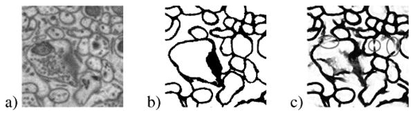
Example of (a) original image, (b) membrane ground truth, and (c) probability map from a supervised learning method showing gaps in the membrane.

Let f be an image initialized from a probability map where 1 represents locations with a low probability of being cell membrane and 0 represents locations with a high probability of being cell membrane. Such a map can come from a supervised classifier. We update f according to the rule f_k+1 = f_k + ∂t(∂f) where

$$\partial f=-\eta {\lambda }_1+\chi {\lambda }_2+\alpha \left|\nabla f\right|\nabla \cdot \frac{\nabla f}{\left|\nabla f\right|}+\beta \nabla f\cdot \nabla G$$ (1)

The ∂t term is a parameter that can be adjusted to improve the stability of the update rule and the η, χ, α, and β terms are parameters that can be used to control how much weight each different term in the PDE has relative to the other terms.

The growth terms in (1) are –ηλ₁ + χλ₂ where λ₁, λ₂ are the eigenvalues of the Hessian matrix of f, and λ₁ > λ₂. The larger eigenvalue of the Hessian of f represents the change across the direction of maximum gradient at each point in f. Figure 2(c) shows that narrow dark structures will have a larger positive value for λ₁ that when subtracted will sharpen membrane structures. As an inverse diffusion, this will effectively bring together areas of wide gray into a narrow dark region over a number of iterations.

Fig. 2.

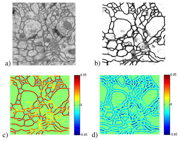
Example of (a) NL-means [10] denoised image, (b) probability map, (c) λ1 map, and (d) λ2 map. Subtracting λ1 darkens the strong membrane areas and adding λ2 pushes out along the edges of the membranes.

The smaller eigenvalue of the Hessian of f represents the change in the direction perpendicular to the direction of the maximum gradient at each point in f. As shown in Figure 2(d) λ₂ is smallest along the edges. When coupled with the image gradient constraint, this will result in directed membrane growth at membrane terminal points which will connect across membrane regions missed in the initial segmentation. In the discrete implementation of the Hessian, central differences are used to compute each of the 2^nd derivatives.

The $\nabla \cdot \frac{\nabla f}{\left|\nabla f\right|}$ term in (1) computes the mean curvature at each pixel location in f [7]. Using the curvature term forces some smoothness along the boundaries between the membrane and non-membrane. Because the cells are generally large rounded structures with few sharp corners, high curvature areas are uncommon resulting in the curvature term favoring objects shaped like the interior of a typical cell. In the discrete implementation of this curvature term, finite central differences are used to compute ∇f.

The final term in (1) has $\nabla G=exp\left(-\frac{|\nabla I{|}^2}{{\sigma }^2}\right)$ where I is a version of the original image filtered with the non-local means algorithm [10] to reduce the effects of noise and blurred with a Gaussian filter to widen the influence of the edges. We chose the non-local means algorithm for noise removal due to its success with textured images. The intent of this term is to push the edges of f to be along the edges of the original image. We assume that there is a strong edge between membrane and non-membrane. Without further constraints this produces a jagged edge because of the noisy nature of the image edges. Combined with the curvature term, the edges of f will produce a cleaner edge that closely follows the edges in the original image. In the discrete implementation of this gradient term, an upwind scheme is used to compute ∇f and finite central differences are used to compute ∇G and ∇I.

Together the curvature and gradient terms provide a means for controlling the inverse diffusion and directed growth terms, but they don't completely control the result to converge to a meaningful solution. To provide a meaningful solution a fixed number of iterations must be selected to achieve the optimal result. Observing the results of this algorithm for a variable number of maximum iterations on a set of different images shows a result where the optimal number of iterations is different for every image. To allow for greater flexibility on the result, we choose a threshold γ below which the locations in f are considered to be membrane and then for each location in f record at which iteration number it reached that threshold.

Once the maximum number of iterations is complete, we take as the result the membrane iteration number divided by the maximum number of iterations. Locations that never reach the threshold are then assigned a value of 1 and are considered to be non-membrane. The result is a confidence map similar to the initialization where 1 represents locations with a low confidence of being cell membrane and 0 represents locations with a high confidence of being cell membrane. The primary consideration in selecting the number of iterations to run is ensuring that it is sufficiently long for all of the small to medium sized membrane gaps to be closed.

One additional constraint that we place on each iteration to control the range is to clip f above and below a certain threshold since the growth term which can create f values that are either less than 0 or greater than 1. We account for these situations by setting all locations where f < 0 to 0 and all locations where f > 1 to 1 at every iteration. Clipping at these values ensures that f remains similar to a probability map throughout all iterations.

3. Results

To test the results of this algorithm we used two different datasets. The first dataset we used for these experiments is a stack of 60 images from a serial section Transmission Electron Microscopy (ssTEM) data set of the Drosophila first in-star larva ventral nerve cord (VNC) [11]. It has a resolution of 4 × 4 × 50 nm/pixel and each 2D section is 512 × 512 pixels. The corresponding binary labels were annotated by an expert neuroanatomist who marked membrane pixels with zero and the rest of pixels with one. During the ISBI Electron Microscopy Image Segmentation Challenge 30 images were used for training and the remaining images were used for testing. For this dataset we will use 2 different probability maps as the initialization point for the PDE to show how the quality of the initialization effects the result of the PDE.

The first probability map we used was generated using multi-scale series artificial neural networks (MSANN) [5]. This map suffers from under segmentation in general but has a fairly low false-positive rate. The second probability map we used was generated using deep neural networks (DNN) [4, 12]. This map was the leading result from the 2012 ISBI Electron Microscopy Image Segmentation Challenge and has very little under-segmentation. The parameters used were optimized empirically using the 30 training images and the remaining 30 images were used as test images. The PDE ran for 1200 iterations with η equal to .3, χ equal to .3, α equal to 0.2, and β equal to 1.2. This places the most weight on the gradient term to balance the growth induced by the inverse diffusion and directed growth terms and minimal weight on the curvature term.

Figure 3 shows the original image, ground truth, MSANN probability map, and resulting image after processing with the PDE. The results for the entire dataset are reported in Table 1 using the 1 minus pair f-score (1 – F) metric. This metric was used in the ISBI 2012 segmentation challenge [13] and is a measure of disagreement in the segmentation. The threshold was chosen to provide the lowest 1 – F.

Fig. 3.

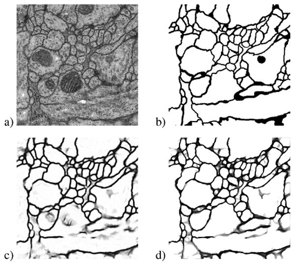
Example of (a) original raw image from the Drosophilia dataset [11], (b) true label, (c) MSANN result, and (d) MSANN+PDE result. Small to medium sized gaps throughout the image are closed and weak membranes are strengthened.

Table 1.

1 – F performance of the PDE on two different probability maps using the Drosophila dataset.

Method	MSANN	MSANN +PDE	DNN	DNN +PDE
Training	0.2084	0.1170	no data	no data
Testing	0.1509	0.1242	0.0504	0.0533

The second dataset used for these experiments is from the mouse neuropil. This set consists of 70 images size 700 × 700× manually annotated by an expert electron microscopist that have been separated into 5 bins with 14 images per bin. 1 bin of 14 images was used in training of the MSANN and the same set of images was used for empirical parameter optimization. The other 4 bins were used as different sets of testing images. There was not a DNN network probability map available for this dataset. For this experiment the same parameters were used as in the Drosophila dataset but for 1400 iterations. The results for this dataset are shown in Figure 4 and Table 2.

Fig. 4.

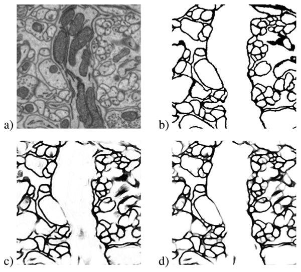
Example of (a) original raw image from the mouse neuropil dataset, (b) true label, (c) MSANN probability map, and (d) results of MSANN + PDE processing. Small to medium sized gaps still closed, but large gaps remain and some oversegmentation is introduced.

Table 2.

1 – F performance of the PDE on different bins of probability maps using the mouse neuropil dataset.

Method	Bin 1	Bin 2	Bin 3	Bin 4	Bin 5
MSANN	0.1626	0.2749	0.2419	0.2115	0.2716
MSANN +PDE	0.1274	0.2226	0.2247	0.1482	0.2196

4. Discussion

Using a PDE we were able demonstrate an ability to close small to medium sized gaps that remain after a supervised learning process has performed initial segmentation of the images. When these types of gaps are prevalent there is a significant improvement in the 1 – F of the result. If the gaps are too large such as in bin 3 of the mouse neuropil dataset or there are very few gaps to close such as with the DNN probability maps on the Drosophila dataset the improvement is not as pronounced. Even in the case of no gaps to close, the 1 – F is not significantly negatively affected by the PDE. This deep convolution example while quite good on it's own, takes one year to train without a GPU cluster [4] making a more efficient alternative desireable. In each of these cases, there is some amount of oversegmentation that results from the processing. This tendency to create oversegmentations prevents running the algorithm for sufficient iterations to close larger gaps. Further improvement of this PDE process could include an additional constraint that prevents oversegmentation or by applying an additional process designed to improve the result of an oversegmentation.

References

- 1.Hayworth KJ, Kasthuri N, Schalek R, Lichtman JW. Automating the collection of ultrathin serial sections for large volume tem reconstructions. Microscopy and Microanalysis. 2006;12(no. Supplement S02):86–87. [Google Scholar]
- 2.Denk W, Horstmann H. Serial block-face scanning electron microscopy to reconstruct three-dimensional tissue nanostructure. PLoS Biol. 2004;no. 2(11):e329. doi: 10.1371/journal.pbio.0020329. 10. [DOI] [PMC free article] [PubMed] [Google Scholar]
- 3.Jain V, Murray JF, Roth F, Turaga S, Zhigulin V, Briggman KL, Helmstaedter MN, Denk W, Seung HS. Supervised learning of image restoration with convolutional networks. ICCV 2007. 2007 Oct.:1–8. [Google Scholar]
- 4.Ciresan DC, Giusti A, Gambardella LM, Schmidhuber J. Deep neural networks segment neuronal membranes in electron microscopy images. NIPS. 2012 [Google Scholar]
- 5.Seyedhosseini M, Kumar R, Jurrus E, Guily R, Ellisman M, Pfister H, Tasdizen T. Detection of neuron membranes in electron microscopy images using multi-scale context and radon-like features. MICCAI 2011. 2011;6891:670–677. doi: 10.1007/978-3-642-23623-5_84. Lecture Notes in Computer Science (LNCS) [DOI] [PMC free article] [PubMed] [Google Scholar]
- 6.Macke J, Maack N, Gupta R, Denk W, Schölkopf B, Borst A. Contour-propagation algorithms for semi-automated reconstruction of neural processes. J of Neuroscience Methods. 2008;167(no. 2):349–357. doi: 10.1016/j.jneumeth.2007.07.021. [DOI] [PubMed] [Google Scholar]
- 7.Caselles V, Ron K, Sapiro G. Geodesic active contours. IJCV. 1997;22:61–79. [Google Scholar]
- 8.Jang DP, Lee DS, Kim SI. Contour detection of hippocampus using dynamic contour model and region growing. EMBS, 1997. 1997 Oct-Nov;2:763–766. [Google Scholar]
- 9.Liu T, Jurrus E, Seyedhosseini M, Ellisman M, Tasdizen T. Watershed merge tree classification for electron microscopy image segmentation. ICPR. 2012 [PMC free article] [PubMed] [Google Scholar]
- 10.Buades A, Coll B, Morel JM. A non-local algorithm for image denoising. CVPR. 2005 Jun;2:60–65. vol. 2. [Google Scholar]
- 11.Cardona A, Saalfeld S, Preibisch S, Schmid B, Cheng A, Pulokas J, Tomančák P, Hartenstein V. An integrated micro- and macroarchitectural analysis of the Drosophila brain by computer-assisted serial section electron microscopy. PLoS Biol. 2010;8(no. 10):e1000502. doi: 10.1371/journal.pbio.1000502. 10. [DOI] [PMC free article] [PubMed] [Google Scholar]
- 12.Ciresan DC, Meier U, Schmidhuber J. Multicolumn deep neural networks for image classification. CVPR. 2012:3642–3649. doi: 10.1016/j.neunet.2012.02.023. [DOI] [PubMed] [Google Scholar]
- 13.Segmentation of neuronal structures in EM stacks challenge - ISBI 2012. [accessed on November 6, 2012]; http://fiji.sc/Segmentation_of_neuronal_structures_in_EM_stacks_challenge_-_ISBI_2012.