Flow disturbances generated by feeding and swimming zooplankton

Significance

Plankton compromise their survival when they swim and feed because the fluid disturbances that they generate may be perceived by predators. Because the abundance and population dynamics of zooplankton in the ocean are governed by their access to food and exposure to predators, an important question is to what extent and how zooplankton may minimize the fluid disturbances that they generate. We show that when swimming and feeding are integrated processes, zooplankton generate fluid disturbances that extend much farther in the water than is the case for zooplankton that swim only to relocate. Quiet swimming is achieved through “breast swimming” or by swimming by jumping, whereas other propulsion modes are much noisier. This pattern applies independent of organism size and species.

Abstract

Interactions between planktonic organisms, such as detection of prey, predators, and mates, are often mediated by fluid signals. Consequently, many plankton predators perceive their prey from the fluid disturbances that it generates when it feeds and swims. Zooplankton should therefore seek to minimize the fluid disturbance that they produce. By means of particle image velocimetry, we describe the fluid disturbances produced by feeding and swimming in zooplankton with diverse propulsion mechanisms and ranging from 10-µm flagellates to greater than millimeter-sized copepods. We show that zooplankton, in which feeding and swimming are separate processes, produce flow disturbances during swimming with a much faster spatial attenuation (velocity u varies with distance r as u ∝ r⁻³ to r⁻⁴) than that produced by zooplankton for which feeding and propulsion are the same process (u ∝ r⁻¹ to r⁻²). As a result, the spatial extension of the fluid disturbance produced by swimmers is an order of magnitude smaller than that produced by feeders at similar Reynolds numbers. The “quiet” propulsion of swimmers is achieved either through swimming erratically by short-lasting power strokes, generating viscous vortex rings, or by “breast-stroke swimming.” Both produce rapidly attenuating flows. The more “noisy” swimming of those that are constrained by a need to simultaneously feed is due to constantly beating flagella or appendages that are positioned either anteriorly or posteriorly on the (cell) body. These patterns transcend differences in size and taxonomy and have thus evolved multiple times, suggesting a strong selective pressure to minimize predation risk.

Zooplankters move to feed, find food, and find mates, so moving is critical to the efficient execution of essential functions. However, moving comes at a predation risk: Swimming increases the predator encounter velocity (encounter rate increases with prey velocity to a power ≤1), and feeding and swimming generate fluid disturbances that may be perceived by rheotactic predators, thus increasing the predator’s detection distance (encounter rate increases with detection distance squared) (1–5). So, the advantages of moving and feeding must be traded off against the associated risks, and organisms should aim at moving and foraging in ways that reduce the predation risk and optimize the trade-off (6, 7). They may do so by moving in patterns that minimize encounter rates (8) and/or they may feed and propel themselves in ways that generate only small fluid disturbances (9). For example, theoretical models suggest that zooplankton that swim by a sequence of jumps may create a smaller fluid disturbance than similar-sized ones that swim smoothly (9), that a hovering zooplankter generates a larger fluid signal than one that cruises through the water (10, 11), and that a zooplankter moving at low Reynolds numbers will generate a relatively larger fluid signal than one moving at higher Reynolds numbers (11). Thus, motility patterns and propulsion modes may strongly influence predation risk and must be subject to strong selection pressure during evolution.

Zooplankton span a huge taxonomic diversity and a large size range (from microns to centimeters) and their propulsion mechanisms vary substantially (12). Unicellular plankton may use one or more flagella or cilia, and the flagella may be smooth or plumose, which has implications for whether the cell is pulled or pushed by the beating flagellum (13). Ciliates may have the cilia rather evenly distributed on the cell surface or concentrated on certain parts of the cell, typically either anteriorly or as an equatorial band. Small animals may have an anterior “corona” of cilia (e.g., rotifers and many pelagic invertebrate larvae) to generate feeding currents and propulsion, or they may have beating or vibrating appendages that can be positioned anteriorly, ventrally, or laterally. The implications and potential adaptive value of this diversity of propulsion modes for feeding and survival are largely unexplored.

Various idealized models, simplifying the swimming organisms to combinations of point forces acting on the water, have been used to describe the fluid disturbance generated by moving and feeding plankton. A self-propelled plankton is often described by a so-called stresslet (two oppositely directed point forces of equal magnitude), a hovering one by a stokeslet (a stationary point force), and a jumping animal by an impulsive stresslet (a stresslet working impulsively) (9, 11, 12). These highly idealized models yield very different predictions of the spatial attenuation of the fluid disturbance and, thus, of how far away the feeding and swimming animal can be detected. A few studies have compared observed flow patterns with those predicted from these simple models and in some cases found fair comparisons (4, 14–17). However, numerical simulations as well as observations of self-propelled microplankton have demonstrated that the distribution of propulsion forces, i.e., the position of flagella, cilia, or appendages on the (cell) body, may have a profound effect on the imposed fluid flow (18, 19). Also, most of the idealized models ignore the fact that swimming in most cases is unsteady, which leads to fluctuating flows at scales smaller than the Stokes length scale ($\sqrt{\nu /\omega }$, where ν is the kinematic viscosity and ω is the beat frequency) (e.g., ref. 19). The simple, idealized models hitherto applied may be insufficient to represent the diverse propulsion modes observed in real organisms and to understand the associated trade-offs.

Feeding and swimming are often part of the same process in zooplankton. Many zooplankton generate a feeding current that at the same time propels the animal through the water. In others, feeding and swimming are separate processes. For example, ambush feeding “sit-and-wait” zooplankters do not move as part of feeding but may swim to undertake vertical migration or to search for mates or patches of elevated food availability. Also, many of the plankton that generate a feeding current by vibrating appendages may in addition swim by using the same appendages in a different way (e.g., the nauplius larvae of most crustaceans) or by using other swimming appendages dedicated to propel themselves (most pelagic copepods and cladocerans).

Whereas feeding and swimming may both compromise the survival of the organism, the trade-offs may be different. To get sufficient food, zooplankters need to daily clear a volume of water for prey that corresponds to about 10⁶ times their own body volume (20, 21) and hence, implicit in the feeding process is the need to examine or process large volumes of water. In contrast, dedicated swimming should translate the organism through the water as quietly as possible. Thus, we hypothesize that in microplankton, dedicated swimming produces flow fields that attenuate more readily and/or have a smaller spatial extension than the cases in which feeding and propulsion are intimately related.

In this study we use particle image velocimetry (PIV) to describe the flow fields generated by micron- to millimeter-sized feeding and swimming zooplankton that use a variety of propulsion modes. We show that—across taxa and sizes—dedicated swimming produces flow fields with a much smaller spatial extension and a faster spatial attenuation than those produced by the plankton for which feeding and swimming are integrated, and we characterize the propulsion modes that minimize susceptibility to rheotactic predators.

Results

The propulsion modes vary substantially between the organisms studied here, in terms of the nature of the propulsion machinery (flagella, cilia, or appendages), the location of the propelling structure on the organism (anteriorly, posteriorly, ventrally, or laterally), the frequency and duration of the power strokes, and the resulting speed and variability in speed (Figs. 1 and 2, Table S1, and Movie S1). These different ways of propelling the organism result in a fascinating diversity of flow fields (Fig. 3 and Movies S2–S4).

Fig. 1.

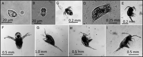
The study organisms with their diverse propulsion equipment. (A–I) The dinoflagellate Oxyrrhis marina (the other dinoflagellates look similar) (A), the ciliate Mesodinium rubrum (B), nauplius of the copepod Acartia tonsa (the nauplius of Temora longicornis looks very similar) (C), the rotifer Brachionus plicatilis (D), the copepod Oithona davisae (E), the cladoceran Podon intermedius (F), the copepod Metridia longa (G), the copepod T. longicornis (H), and the copepod A. tonsa (I).

Fig. 2.

(A–E) Temporal fluctuations in area of influence, S_{0.1 mm/s}, for the dinoflagellate O. marina (A); peak propulsion speed (B); speed variability index (C); area of influence, S_{0.5 mm/s} during the peak of the power stroke (D); and power of spatial flow attenuation (E), all as a function of Reynolds number for swimmers (red symbols and lines) and feeders (blue symbols and lines). The regression lines in D are as follows: swimmers, Log(S, mm²) = −1.54 + 1.36 Log(Re); feeders, Log(S, mm²) = −0.48 + 1.61 Log(Re). Speed variability index is estimated as the difference between peak and average speed divided by the length of the organism. All data are reported in Table S1.

Fig. 3.

Examples of snapshots of flow fields generated by swimming and feeding zooplankton. (A–F) Swimming Oxyrrhis marina (A), nauplius of Temora longicornis producing feeding current (B), swimming Podon intermedius (C), cruising Metridia longa (D), hovering T. longicornis (E), and repositioning jump of Acartia tonsa (F). The position of the organisms is indicated by red ellipses and the swimming direction by white arrows (gray arrow for the hovering T. longicornis). Flow field animations for all species examined are shown in Movies S2–S4.

The dinoflagellates (20–50 µm) all swim by beating two flagella, a longitudinal, trailing flagellum that propels the cell through the water and a transverse flagellum that accounts for rotation and steering of the cell (22). The beating of the trailing flagellum creates a succession of short-lasting, counterrotating vorticity structures in the wake of the cell (Fig. 3A) and a highly fluctuating extension of the flow field (Fig. 2A). The rotifer Brachionus plicatilis (25–50 µm) generates a feeding current and is pulled through the water by cilia organized in frontal coronas that propel constantly (Movie S1); the resulting propulsion speed is near constant (Table S1) and the flow field is almost stationary in time and consists of two vortex rings, one around the translating body and another one of opposite direction around the feeding current (Movie S2). The nauplius (larval stage) of the copepod Temora longicornis (200–300 µm) creates very different flow fields, depending on whether it vibrates its three pairs of appendages to generate a feeding current, or it swims by powerful backward strokes of the appendages (Movie S3). The latter flow field is similar to that produced by the swimming nauplii of the copepod Acartia tonsa (140–240 µm) as well as by the ciliate Mesodinium rubrum (25 µm) and the much larger cladoceran, Podon intermedius (0.7–1.0 mm): The flow both anterior and posterior to the organism is in the swimming direction, whereas the flow lateral to the organism is directed backward (Fig. 3 and Movies S2 and S3). These organisms all “breast-stroke swim” by beating the laterally positioned appendages or cirri backward. The copepodites of the three calanoid copepods all swim and feed by vibrating the anterior-ventrally positioned five pairs of feeding appendages in a rhythmic but convoluted pattern, but the flow fields differ, depending on whether the animal is “hovering,” i.e., generates a feeding current while itself remaining stationary and tethered by gravity (T. longicornis, 0.75 mm), or is cruising through the water (Metridia longa, 2.5 mm) (Fig. 3 C and E). The third calanoid copepod, A. tonsa (0.8 mm) is intermediate between the other two in that it simultaneously swims through the water and generates a feeding current (Movie S4), but it also differs in that it vibrates both its feeding appendages and its swimming legs when generating the current and propelling itself (Movie S1). Finally, all of the copepods can swim by sequentially kicking the four to five pairs of ventrally positioned swimming legs backward, either once or a few times (a repositioning jump: A. tonsa, Oithona davisae females), repeatedly at a high frequency (escape jump, none analyzed), or repeatedly at a lower frequency (swimming by jumping: O. davisae males). In all cases, and best illustrated by A. tonsa (Fig. 3B and Movie S4), two ephemeral vortex rings form, one in the wake of the animal and one around its forward-moving body. A simple categorization of the swimming and feeding behaviors described above is presented in Table 1.

Table 1.

Plankton swimming behaviors, their purposes, and bulk properties of the induced flows

Behavior	Purpose	Species/groups	Idealized model	Spatial attenuation*
Hover	Feeding	T. longicornis copepodite	Stokeslet	r−1
Cruise	Feeding and locomotion	M. longa, dinoflagellates	Stresslet	r−2
Hover/cruise	Feeding and locomotion	B. plicatilis, A. tonsa copepodite feeding, T. longicornis nauplii feeding	Stokeslet+stresslet	r−1 to r−2
Breast-stroke swim	Locomotion	M. rubrum, P. intermedius, nauplii swimming	Potential dipole	r−3
Jumping	Locomotion	Copepods swimming by jumping	Impulsive stresslet	r−4

^*Describes how flow velocity scales with the distance, r, from the swimming plankton. The exponent is that predicted from the idealized models (SI Text) and approximated by the observations (Table S1 and Fig. 4 of the main text).

Ignoring details in the flow structures and focusing on how bulk-induced flow velocity attenuates with distance to the organism, striking patterns emerge (Fig. 4, Table 1, and Table S1). For most species the imposed flow velocity is variable in time. The temporal variation in flow velocity is highest for small organisms and very near the body of the organisms, whereas at distances approaching or exceeding the Stokes length scale, the flow field is more constant in time. As a consequence, the spatial attenuation of the flow field is variable (Fig. 4). However, in the far field, and at the peak of the power stroke, the spatial attenuation tends toward a constant power relationship that is characteristic of each of the flow fields examined and robust to whether the organism is viewed from the dorsal, ventral, or lateral side (Fig. 4 and Table S1). For the zooplankton that swim independent of feeding, the spatial attenuation of the flow is fast and attenuates with distance to power near −4 for the ones that move by jumps (all of the copepods) and near −3 for those that have the swimming appendages organized laterally (the copepod nauplii, P. intermedius and M. rubrum). For those organisms and propulsion modes where swimming and feeding are intimately associated, the spatial attenuation is slower, with powers of between −2 and −1. The copepodite of A. tonsa deviates from this pattern in that its feeding current attenuates rapidly. The flow attenuation is related to, but not well predicted by, the Reynolds number of the moving organism (Fig. 2E) and organisms moving at the highest Reynolds numbers (Re > 10) show almost the full range of spatial attenuations. Thus, the propulsion mode is more relevant than the magnitude of Re for the imposed flow pattern.

Fig. 4.

Examples of the spatial attenuation of flow velocities. (A–H) A. tonsa copepodite repositioning jump (A), O. davisae female repositioning jump (B), P. intermedius swimming (C), A. tonsa nauplii swimming (D), M. longa cruise feeding (E), O. marina cruise feeding (F), T. longicornis nauplius feeding(G), and T. longicornis hovering (H). The solid circles show the attenuation at the peak of the power stroke and the open circles the attenuation during the time leading up to the peak at times given in milliseconds. The solid lines have slopes between −1 and −4 and were adjusted to line up with the far field flow attenuation at the peak of the power stroke. A characteristic far field flow attenuation was somewhat subjectively assigned to each experiment based on how well it compares with the observations; for observations that were between two integer values, we assigned an intermediate value.

As a consequence of the differences in spatial attenuation, the spatial extensions of the flow fields differ (Fig. 2D). Here, we define the spatial extension of the flow field, S, as the peak cross-sectional area within which the imposed fluid velocity exceeds a certain threshold velocity. We have chosen a critical velocity of 0.5 mm⋅s⁻¹: This overlaps with or is close to the highest velocities produced by the smallest organisms examined and the lowest velocities measurable for the largest organisms. In the case of no overlap, we extrapolated from observations, using the estimated power of the spatial attenuation. The resulting area of course depends on the chosen threshold, but the pattern is robust to the choice of threshold: The area of the flow field increases with the Reynolds number of the organism and is nearly an order of magnitude larger for plankton that feed and swim simultaneously compared with those where feeding and swimming are separate processes. In organisms for which we have recordings of both feeding and pure swimming modes, e.g., nauplii of T. longicornis and copepodites of A. tonsa, one can see that they can increase their peak propulsion speed by more than one order of magnitude without (A. tonsa) or by only slightly (factor of 2.3, T. longicornis) increasing the spatial extension of the flow field, as defined above (Fig. 4 and Table S1).

Discussion

Our observations suggest that for plankton that swim to relocate, propulsion has been optimized to minimize the fluid disturbance that they generate, whereas for plankton in which swimming is constrained by a simultaneous need to feed, the fluid disturbance generated is manyfold higher with a consequently higher risk of being detected by a rheotactic predator. Because rheotactic predators respond to imposed fluid velocity magnitude rather than shear (23), the area of influence can be thought of as the encounter cross section toward a rheotactic predator and thus scales directly with predator encounter rate. The threshold velocity of 0.5 mm⋅s⁻¹ was chosen for practical reasons (see above) and a threshold on the order of 0.1 mm⋅s⁻¹ would be more in line with typical threshold flow velocities for prey detection in planktonic predators (21), and such a threshold yields an even larger difference between swimmers and feeders. The higher risk associated with feeding than with pure swimming, of course, may be warranted by the benefits of feeding, and thus plankton are no different from many other organisms that have to compromise their survival to acquire food (6).

What are the characteristics of “quiet” propulsion in contrast to “noisy” feeding and swimming and how do the swimmers reduce the spatial extension of their fluid disturbance? The propulsion speed in almost all of the organisms examined is unsteady due to the beating of appendages or flagella but the size-dependent beat frequencies do not differ significantly between the swimmers and feeders (Table S1). However, the power strokes are shorter in pure swimmers, their peak speeds as well as variability in speed are much larger than in similar-sized feeders, and their propulsion is consequently much more erratic (Fig. 2C, Table S1, and Movie S1). The higher Reynolds numbers of the swimmers than those of equal-sized feeders can only partly account for the limited extension of their flow fields. We have previously shown for swimming plankton that if the power stroke is short relative to the Stokes timescale, the flow structure formed may be characterized by two viscous vortex rings with a fast spatial and temporal attenuation (9). All of the jumping and swimming copepods in fact produce two such vortex rings (Fig. 3 and Movies S2–S4) consistent with previous observations in different species (4, 17, 24), and the observed far field spatial attenuation of the flow (u ∼ r^-4) is consistent with that predicted from the idealized impulsive stresslet model (Table 1). Thus, the rapid power strokes may be considered an adaptation to minimize the production of fluid signals.

None of the other swimmers examined, the ciliate (M. rubrum), the copepod nauplii (A. tonsa and T. longicornis), and the cladoceran (P. intermedius), form similar vortex rings, but they are all “breast swimmers” with the propulsion apparatus positioned (bi)laterally symmetrically (Fig. 1 and Movie S1) and with quite similar flow fields (Movies S2–S4). The far field flow generated by them resembles that of a potential dipole (SI Text, Figs. S1–S4, and Tables S2–S5). A potential dipole can physically be thought of as a fluid point sink and a fluid point source, with strengths of equal magnitude m, to be placed at two points separated by a distance δ in such a way that m × δ remains constant when the separation δ vanishes (25). A potential dipole is mathematically equivalent to a magnetic dipole. The striking swimming appendages follow rather well the streamlines of a potential dipole (equivalent to the magnetic field lines) (SI Text and Movie S5), which explains the similarities of the flows. Bulk properties of the flows are also similar in that the observed far field flow attenuation for these swimmers is close to that predicted by the potential dipole (u ∼ r^-3) and the flow fields, streamlines, and velocity magnitudes are well predicted by the potential dipole model (SI Text). A previous computational fluid dynamics simulation study of the ciliate M. rubrum has similarly shown a dipole-like flow pattern and ∼r⁻³ flow attenuation (26). Breast swimming can thus be considered an adaptation to minimize the fluid disturbances of swimming plankton. Its existence over a large size range and in diverse taxa suggests that this body plan and this propulsion mode have evolved multiple times in the course of evolution. Note that the nauplius is the characteristic pelagic larva not only of copepods but of many crustaceans, an abundant and widespread animal group in the ocean, and the nauplius has been characterized as one of the most successful larval forms in the pelagic environment (27).

The zooplankton that feed and swim simultaneously cruise through the water (M. longa, the dinoflagellates), hover in an almost stationary position while producing a feeding current (T. longicornis copepodite), or do something in between, i.e., translating through the water and simultaneously drawing water toward themselves (all of the others). With the exception of A. tonsa copepodites, their observed far field spatial attenuation of the flow fields scales with the distance to powers between −1 and −2, comparable to that predicted by the idealized stokeslet (hovering, −1) and stresslet (cruising, −2) models (SI Text).

There is an additional consistent taxa-transcending difference between swimmers and feeders that allows the swimmers to further reduce their susceptibility to rheotactic predators: The swimmers swim intermittently, whereas the feeders feed and swim almost continuously—a difference that applies generally and not only to the study organisms. The frequency of reposition jumps in copepods and ciliates is between 1.0 s⁻¹ and 0.01 s⁻¹ (28, 29) (reviewed in ref. 4) with each jump lasting only a few milliseconds. The males of the copepod Oithona spp. swim for only about one-third of the time (30) and the actual swimming takes up only a fraction of that time. The cladocerans similarly have long breaks between swimming events. In contrast, flagellates, most ciliates, rotifers, nauplii, and copepods that generate a feeding current or cruise while feeding do so almost continuously (10, 28, 31). Because the swimmers propel faster than the feeders, the total distance they cover per unit time, and hence the average predator encounter velocity, may not be different between swimmers and feeders, but the swimmers produce only small ephemeral flow structures and are “invisible” to rheotactic predators for most of the time.

The copepod A. tonsa is different from the other feeding copepods, in that its flow field attenuates faster than predicted by the idealized models. It also differs in the way it produces the feeding current by vibrating both the feeding and the swimming appendages, as has been observed in other species of the genus (32), and it feeds only intermittently and for only 5–20% of the time (33). This suggests that its feeding current is very efficient and that its exposure to rheotactic predators is limited, which in turn may account for the evolutionary success of this particular family, as judged both from its numerical dominance in neritic plankton communities around the world and from its capacity to colonize new areas (34–37).

Propulsion strategy may be adapted to optimize a variety of functions. Hitherto propulsion and feeding in zooplankton have mainly been examined from the perspective of food acquisition and propulsion energetics (12), but optimization of feeding and propulsion should not only consider the energetics but also take inescapable predation risk into account (3). Our study suggests that predation is a strong selective agent in shaping the motility and propulsion strategy of zooplankton and that these organisms can substantially reduce their susceptibility to rheotactic predators as they swim when they are not constrained by a simultaneous need to gather food.

Methods

Most experimental organisms were taken from our laboratory cultures. Exceptions were the copepod Metridia longiremis that was collected in Disko Bay, Greenland, and the cladoceran P. intermedius that we collected in Gulmar Fjord, Sweden. We used PIV to visualize 2D transects of the fluid flow generated by swimming plankton. Briefly, swimming and/or feeding zooplankters were filmed with a high-resolution (1,280 × 800 pixels), high-speed (100–2,200 frames⋅s⁻¹) Phantom V210 video camera. The camera was equipped with lenses to produce appropriate fields of view (i.e., such that the entire extension of the flow field was covered), from 0.28 × 0.17 mm² for the smallest flagellates to 28 × 17 mm² for the largest copepods. Copepods (nauplii and copepodites) and cladocerans swam in small aquaria, varying in size from 1 × 1 × 4 cm³ (nauplii and small copepodites) and 5 × 5 × 5 cm³ (small copepods and cladocerans) to 8.5 × 10.2 × 3.2 cm³ (large copepods).

Protists swam in ∼0.5-mm high, 10-mm radius chambers mounted on a microscopic slide. In all cases the fluids were seeded with tracer particles to visualize the flow, 0.5-µm polymer microspheres for the protists and 5- to 10-µm hollow glass spheres or ∼1-µm titanium oxide particles for the larger organisms. Illumination was provided by a pulsed infrared laser (808 nm) that was synchronized with the camera and passed through optics to produce a thin sheet (150–300 µm). The camera was oriented perpendicular to the laser sheet. The dinoflagellates, the rotifer, and the copepod nauplii were filmed in an inverted microscope. In this case the depth of the narrow focal plane rather than a laser sheet defined the thickness of the flow structure recorded. We selected short movie sequences (40–500 frames) where the organisms moved in the focal plane or in the plane of the laser sheet. Because the imaging is in 2D and swimming is in 3D, this is a potential source of variation, but we minimized this variation by selecting sequences where the peak estimates of the spatial extension of the flow field (see below) were constant in time (i.e., not increasing or decreasing). These sequences were analyzed using DaVis PIV software to get quantitative descriptions of the temporal variation of the flow field generated by the swimming/feeding organism. We quantified the spatial extension of the flow by measuring the area, S(U*), within which the induced flow velocity exceeds a threshold value, U*, for different values of U*. Velocity estimates were made at a resolution of 16 pixels × 16 pixels, and S(U*) was estimated as the fraction of squares with velocity estimates exceeding U* multiplied by the area of the field of view. We describe the spatial attenuation of the flow by plotting U* as a function of the equivalent circular radius of that area. We did not mask the organisms before extracting the flow fields, and the motion of the organism itself thus appears as induced water motion. The reasons for not masking are twofold: (i) We focus on the far field flow and hence a correct description of the near field is of less importance, and (ii) by not masking we correctly estimate the area influenced by the organism. For presentation purposes, and to visualize the near field flow, we masked the animals (Fig. 3 and Movies S2–S5). We computed the body Reynolds number of the feeding and swimming organisms as $Vl/\nu$, where V is the peak velocity of the animal relative to the fluid (i.e., its swimming velocity plus the oppositely directed component of feeding current velocity, both measured relative to the camera), l is the body length of the organism, and ν is the kinematic viscosity. The swimming speeds of the organisms were obtained by digitizing their position in subsequent frames. We also computed an index of the relative variability in swimming speed, as the peak minus the average speed divided by the length of the organism. To describe the propulsion modes of the different organisms we filmed them in the absence of PIV particles, using optimal illumination (Movie S1). We either shone infrared light through the swimming aquarium toward the camera or used the light provided by the microscope.

References

- 1.Evans GT. The encounter speed of moving predator and prey. J Plankton Res. 1989;11:415–417. [Google Scholar]
- 2.Visser AW. Motility of zooplankton: Fitness, foraging and predation. J Plankton Res. 2007;29:447–461. [Google Scholar]
- 3.Gerritsen J, Strickler JR. Encounter probabilities and community structure in zooplankton. Mathematical model. J Fish Res Bd Can. 1977;34(1):73–82. [Google Scholar]
- 4.Kiørboe T, Jiang H, Colin SP. Danger of zooplankton feeding: The fluid signal generated by ambush-feeding copepods. Proc Biol Sci. 2010;277(1698):3229–3237. doi: 10.1098/rspb.2010.0629. [DOI] [PMC free article] [PubMed] [Google Scholar]
- 5.Tiselius P, Jonsson PR, Kaartvedt S, Olsen ME, Jarstad T. Effects of copepod foraging behavior on predation risk: An experimental study of the predatory copepod Pareuchaeta norvegica feeding on Acartia clausi and A. tonsa (Copepoda) Limnol Oceanogr. 1997;42(1):164–170. [Google Scholar]
- 6.Houston AI, McNamara JM, Hutchinson JMC. General results concerning the trade-off between gaining energy and avoiding predation. Philos Trans R Soc Lond B Biol Sci. 1993;341:375–397. [Google Scholar]
- 7.Lima S, Dill LM. Behavioral decisions made under the risk of predation: A review and prospectus. Can J Zool. 1990;68:619–640. [Google Scholar]
- 8.Visser AW, Kiørboe T. Plankton motility patterns and encounter rates. Oecologia. 2006;148(3):538–546. doi: 10.1007/s00442-006-0385-4. [DOI] [PubMed] [Google Scholar]
- 9.Jiang H, Kiørboe T. The fluid dynamics of swimming by jumping in copepods. J R Soc Interface. 2011;8(61):1090–1103. doi: 10.1098/rsif.2010.0481. [DOI] [PMC free article] [PubMed] [Google Scholar]
- 10.Tiselius P, Jonsson P. Foraging behavior of 6 calanoid copepods – observations and hydrodynamic analysis. Mar Ecol Prog Ser. 1990;66:23–33. [Google Scholar]
- 11.Visser AW. Hydromechanical signals in the plankton. Mar Ecol Prog Ser. 2001;222:1–24. [Google Scholar]
- 12.Guasto JS, Rusconi R, Stocker R. Fluid mechanics of plankton microorganisms. Annu Rev Fluid Mech. 2012;44:373–400. [Google Scholar]
- 13.Christensen-Dalsgaard KK, Fenchel T. Complex flagellar motions and swimming patterns of the flagellates Paraphysomonas vestita and Pteridomonas danica. Protist. 2004;155(1):79–87. doi: 10.1078/1434461000166. [DOI] [PubMed] [Google Scholar]
- 14.Catton KB, Webster DR, Brown J, Yen J. Quantitative analysis of tethered and free-swimming copepodid flow fields. J Exp Biol. 2007;210(Pt 2):299–310. doi: 10.1242/jeb.02633. [DOI] [PubMed] [Google Scholar]
- 15.Drescher K, Goldstein RE, Michel N, Polin M, Tuval I. Direct measurement of the flow field around swimming microorganisms. Phys Rev Lett. 2010;105(16):168101. doi: 10.1103/PhysRevLett.105.168101. [DOI] [PubMed] [Google Scholar]
- 16.Kiørboe T, Jiang H. To eat and not be eaten: Optimal foraging behavior in suspension feeding copepods. J R Soc Interface. 2013;10(78):20120693. doi: 10.1098/rsif.2012.0693. [DOI] [PMC free article] [PubMed] [Google Scholar]
- 17.Murphy DW, Webster DR, Yen J. A high-speed tomographic PIV system for measuring zooplanktonic flow. Limnol Oceanogr Methods. 2012;10:1096–1112. [Google Scholar]
- 18.Jiang H, Paffenhöfer G-A. Hydrodynamic signal perception by the copepod Oithona plumifera. Mar Ecol Prog Ser. 2008;373:37–52. [Google Scholar]
- 19.Guasto JS, Johnson KA, Gollub JP. Oscillatory flows induced by microorganisms swimming in two dimensions. Phys Rev Lett. 2010;105(16):168102. doi: 10.1103/PhysRevLett.105.168102. [DOI] [PubMed] [Google Scholar]
- 20.Hansen PJ, Bjørnsen PK, Hansen BW. Zooplankton grazing and growth: Scaling within the 2-2,000-mu m body size range. Limnol Oceanogr. 1997;42:35687–35704. [Google Scholar]
- 21.Kiørboe T. How zooplankton feed: Mechanisms, traits and trade-offs. Biol Rev Camb Philos Soc. 2011;86(2):311–339. doi: 10.1111/j.1469-185X.2010.00148.x. [DOI] [PubMed] [Google Scholar]
- 22.Fenchel T. How dinoflagellates swim. Protist. 2001;152(4):329–338. doi: 10.1078/1434-4610-00071. [DOI] [PubMed] [Google Scholar]
- 23.Kiørboe T, Visser AW. Predator and prey perception in copepods due to hydromechanical signals. Mar Ecol Prog Ser. 1999;179:81–95. [Google Scholar]
- 24.Yen J, Strickler JR. Advertisement and concealment in the plankton: What makes a copepod hydrodynamically conspicuous? Inv Biol. 1996;115(3):191–205. [Google Scholar]
- 25.Batchelor GK. An Introduction to Fluid Dynamics. Cambridge, UK: Cambridge Univ Press; 1967. [Google Scholar]
- 26.Jiang H. Why does the jumping ciliate Mesodinium rubrum possess an equatorially located propulsive ciliary belt? J Plankton Res. 2011;33:998–1011. [Google Scholar]
- 27.Martin JW, Olesen J, Høeg JT. The nauplius. In: Martin JW, Olesen J, Høeg JT, editors. Atlas of Crustacean Larvae. Baltimore: Johns Hopkins Univ Press; 2014. pp. 8–16. [Google Scholar]
- 28.Buskey EJ, Coulter C, Strom S. Locomotory patterns of microzooplankton: Potential effects on food selectivity of larval fish. Bull Mar Sci. 1993;53(1):29–43. [Google Scholar]
- 29.Fenchel T, Hansen PJ. Motile behaviour of the bloom-forming ciliate Mesodinium rubrum. Mar Biol Res. 2006;2:33–40. [Google Scholar]
- 30.Kiørboe T. Optimal swimming strategies in mate-searching pelagic copepods. Oecologia. 2008;155(1):179–192. doi: 10.1007/s00442-007-0893-x. [DOI] [PubMed] [Google Scholar]
- 31.Titelman J, Kiørboe T. Motility of copepod nauplii and implications for food encounter. Mar Ecol Prog Ser. 2003;247:123–135. [Google Scholar]
- 32.Rosenberg G. Filmed observations of filter-feeding in the marine planktonic copepod Acartia clausi. Limnol Oceanogr. 1980;25:738–742. [Google Scholar]
- 33.Jonsson P, Tiselius P. Feeding behaviour, prey detection and capture efficiency of the copepod Acartia tonsa feeding on planktonic ciliates. Mar Ecol Prog Ser. 1990;60:35–44. [Google Scholar]
- 34.Durbin EG, Durbin AG, Smayda TJ, Verity PG. Food limitation of production by adult Acartia tonsa in Narragansett Bay, Rhode Island. Limnol Oceanogr. 1983;28:1199–1213. [Google Scholar]
- 35.Hoffmeyer M. Decadal change in zooplankton seasonal succession in the Bahía Blanca estuary, Argentina, following introduction of two zooplankton species. J Plankton Res. 2004;26(2):181–189. [Google Scholar]
- 36.David V, Sautour B, Chardy P. Successful colonization of the calanoid copepod Acartia tonsa in the oligo-mesohaline area of the Gironde estuary (SW France) – Natural or anthropogenic forcing? Estuar Coast Shelf Sci. 2007;71:429–442. [Google Scholar]
- 37.Aravena G, Villate F, Uriarte I, Iriarte A, Ibáñez B. Response of Acartia populations to environmental variability and effects of invasive congenerics in the estuary of Bilbao, Bay of Biscay. Estuar Coast Shelf Sci. 2009;83:621–628. [Google Scholar]
Associated Data
This section collects any data citations, data availability statements, or supplementary materials included in this article.