In situ determination of alveolar septal strain, stress and effective Young's modulus: an experimental/computational approach

Abstract

Alveolar septa, which have often been modeled as linear elements, may distend due to inflation-induced reduction in slack or increase in tissue stretch. The distended septum supports tissue elastic and interfacial forces. An effective Young's modulus, describing the inflation-induced relative displacement of septal end points, has not been determined in situ for lack of a means of determining the forces supported by septa in situ. Here we determine such forces indirectly according to Mead, Takishima, and Leith's classic lung mechanics analysis (J Appl Physiol 28: 596–608, 1970), which demonstrates that septal connections transmit the transpulmonary pressure, P_TP, from the pleural surface to interior regions. We combine experimental septal strain determination and computational stress determination, according to Mead et al., to calculate effective Young's modulus. In the isolated, perfused rat lung, we label the perfusate with fluorescence to visualize the alveolar septa. At eight P_TP values around a ventilation loop between 4 and 25 cmH₂O, and upon total deflation, we image the same region by confocal microscopy. Within an analysis region, we measure septal lengths. Normalizing by unstressed lengths at total deflation, we calculate septal strains for all P_TP > 0 cmH₂O. For the static imaging conditions, we computationally model application of P_TP to the boundary of the analysis region and solve for septal stresses by least squares fit of an overdetermined system. From group septal strain and stress values, we find effective septal Young's modulus to range from 1.2 × 10⁵ dyn/cm² at low P_TP to 1.4 × 10⁶ dyn/cm² at high P_TP.

inflation-induced alveolar septal elongation is a major determinant of alveolar expansion (15), and thus lung ventilation. Alveolar septa are nearly planar tissue structures lined on each side by a thin liquid layer (6, 16). Septal cross sections have often been modeled as linear elements (e.g., Refs. 2, 11, 25). In such modeling, it would be valuable to know the effective Young's modulus, E_Eff, for the in situ septum as a function of transpulmonary pressure, P_TP. An effective modulus would capture inflation-induced septal distension, whether due to reduced slack or increased tissue stretch. An effective modulus would incorporate tissue elastic and interfacial forces, both of which are supported by the in situ septum (Fig. 1). The effective modulus would not represent a material property but, rather, describe net septal elongation in response to lung inflation. Without a means of determining septal force inside the intact lung, however, E_Eff values have not been determined.

Fig. 1.

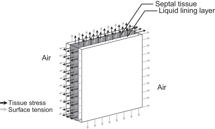
Forces acting on a section of in situ alveolar septum. Alveolar septal tissue (gray) is lined on each side by a thin liquid layer (white). The combined tissue/liquid structure is surrounded by air. At sections through the septum (all 4 edges), tissue stress acts throughout the tissue and surface tension at the air-liquid interface.

Given the difficulty of accessing the interior of the intact lung, the mechanics of isolated lung tissue structures have been tested in vitro. Stress-strain relations have been determined for lung tissue samples 200 μm in length (4). In larger tissue strips, tissue and extracellular matrix moduli have been determined at zero strain by atomic force microscopy (8, 9) and tissue Young's modulus has been estimated from the uniaxial stress-strain relation (2). Atomic force microscopy data, in particular, are valuable for their high spatial resolution. As informative as in vitro studies are, however, surface tension is absent in vitro. Surface tension contributes to the effective in situ septal modulus and may also, by modulating extracellular matrix distension, alter septal tissue modulus (6). Furthermore, measurements in isolated lung structures do not enable determination of the relation between modulus and P_TP. In characterizing lung mechanics, it is important to determine modulus within the physiological range of P_TP values and know the P_TP at which a given modulus value applies.

Here, we determine in situ septal forces indirectly by application of Mead, Takishima, and Leith's classic demonstration (12) that the P_TP is transmitted without distortion to and maintains inflation of interior lung regions. That is, P_TP acts directly only across the pleural surface; inside the lung, the same pressure, alveolar pressure, acts on both sides of a given septum. Yet for any interior lung region there are paths of connected septa that radiate away from the region and tether it to the pleura. These septal paths transmit the P_TP from the pleura into the lung. An increase in P_TP expands interior lung regions as though the P_TP were acting directly upon them.

We employ Mead et al.'s model to determine effective alveolar Young's modulus as follows. Imaging a lung region by confocal microscopy at a sequence of P_TP values that constitute a full ventilation loop, and upon total deflation, we determine septal strains within an analysis region. At each point on the ventilation loop, we simulate direct application of P_TP to the boundary of the analysis region. Within the analysis region, alveolar geometries are known. By force balance, we determine stresses in all septa within the region. From experimentally determined strain and computationally determined stress, we derive an effective Young's modulus that describes the typical alveolar septal response to lung inflation.

METHODS

To determine alveolar septal strain and stress in situ, we combine experimental and computational methods.

Experimental determination of septal strain.

In the isolated, perfused rat lung, we label the perfusate with fluorescence for alveolar septal visualization and length determination by confocal microscopy (15, 27). Briefly, in accord with a protocol approved by the Stevens Institute of Technology Institutional Animal Care and Use Committee, we anesthetize male Sprague-Dawley rats (n = 3, 340–360 g) with 1.5–4% isoflurane (Penn Veterinary Supply, Lancaster, PA) in oxygen. We puncture the heart through the chest wall, inject 1,500 U/kg heparin (Penn Veterinary Supply) and withdraw >10 ml of blood. We perform a tracheotomy and cannulate the trachea. We perform a sternotomy, cannulate the pulmonary artery via the right ventricle, cannulate the left atrium via the left ventricle and excise the heart and lungs en bloc. We inflate the lungs to a P_TP of 30 cmH₂O/total lung capacity (TLC) and then deflate to a P_TP of 4 cmH₂O/functional residual capacity (FRC) (19). We connect the cardiac cannulas to a perfusion circuit and pump 10 ml of autologous blood plus 18 ml of 5% albumin (Sigma Aldrich, St. Louis, MO) in normal saline through the lungs, at 9 ml/min and 37°C. We maintain left atrial pressure at 3 cmH₂O. At P_TP of 5 cmH₂O, pulmonary arterial pressure is 10 cmH₂O. For visualization of the alveolar septa, we fluorescently label the vasculature within the septa by addition of 23 μM fluorescein (Cole Parmer, Vernon Hills, IL) to the perfusate. Following fluorescent labeling of the vasculature, we stop perfusion and disconnect the perfusion circuit from the cardiac cannulas, which are left open ended. It is to avoid the possibility of generating alveolar edema that we perfuse at a low flow rate and then arrest perfusion. Despite the lack of vascular pressure, perfusion arrest does not detectably alter septal thickness or alveolar mechanics (27).

We image fluorescently labeled septa on the costal surface of the lower left lobe by confocal microscopy (SP5, Leica Microsystems, Buffalo Grove, IL). We use an ×20 (0.5 N.A.) water immersion objective, and an O-ring-mounted coverslip to support a water drop for objective immersion (27). With the coverslip positioned just in contact with a thin film of saline solution atop the lung surface, the coverslip does not alter alveolar geometry or mechanics (27). At a given P_TP, we collect a z-stack of optical sections (0.28/0.36 μm pixel length for P_TP = 0 cmH₂O/P_TP > 0 cmH₂O; 3.5 μm optical section thickness; 2.5 μm center-to-center distance between sequential sections) from the pleural surface to a depth of 30 μm. The optical sections are aligned with the x–y plane, parallel to the pleural surface; the depth of their thickness is measured along the z-axis, perpendicular to the pleural surface. We excite and collect fluorescence at 488 and 500 (high pass) nm, respectively.

We image the same alveolar field at a sequence of eight P_TP values around a ventilation cycle, according to the following protocol. We remove the coverslip and ventilate the unrestrained lung twice at 0.33 Hz between P_TP of 4 and 25 cmH₂O. We then arrest ventilation, hold the lung at constant P_TP of 4 cmH₂O, replace the coverslip, and acquire a z-stack of confocal images. The time between ventilation arrest and commencement of imaging, the total imaging time, and the total time of ventilation arrest are ∼2, 1.7, and 5.5 min, respectively. We repeat the procedure (two dynamic ventilation loops, then stop and hold the lung at constant pressure for imaging) for each of the following P_TP: 6 inflation, 9 inflation, 15 inflation, 25, 15 deflation, 9 deflation, and 6 deflation cmH₂O. Finally, we deflate the lung to P_TP of 0 cmH₂O for imaging in the unstressed state.

We determine alveolar strain in one optical section from the z-stack obtained at each P_TP, performing our analysis in ImageJ (NIH, Bethesda, MD). At P_TP of 4 cmH₂O, we perform our analysis in an optical section located 22 ± 2 μm below the pleural surface. For all other P_TP, we use morphological landmarking to identify the corresponding optical section, as described previously (15). From P_TP of 4 to 25 cmH₂O, subpleural depth of the analyzed plane increases by 6 μm, indicating alveolar expansion in the z-direction. Across all P_TP, we place a node at the center of each three-way (and the occasional four-way) septal junction. We connect the nodes with straight-line elements and use the lengths of the elements, L_Sept, to approximate septal lengths. Figure 2 shows images of and model elements for one alveolar region over a range of P_TP.

Fig. 2.

Septal element model. Top: confocal microscopy images of fluorescently labeled vasculature in subpleural alveoli of isolated, perfused rat lung, at 4 transpulmonary pressure, P_TP, values, on deflation. At P_TP of 4 cmH₂O, subpleural depth is 24 μm. Bottom: same images with overlay of alveolar element model. Alveolar septa are represented by linear elements: red on periphery of region to be analyzed, white in interior. Dashed elements indicate cross-bridge structures that arch over the tops of alveoli.

The orientation of subpleural septa tends to be uniform. These septa typically meet the pleural surface at a right angle, as shown in Fig. 3A. Some subpleural alveoli, however, have arch structures over their top surface (Fig. 3B). Forces supported by these arch structures have components within the plane of our analysis. When such an arch structure is evident as a “cross bridge” in the x–y plane of analysis at P_TP of 4 cmH₂O, we include the cross bridge as a septal element (Fig. 2, dashed lines) in our model. Unless otherwise noted, however, we omit cross-bridge elements when reporting the results of our analysis.

Fig. 3.

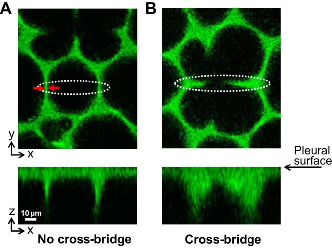
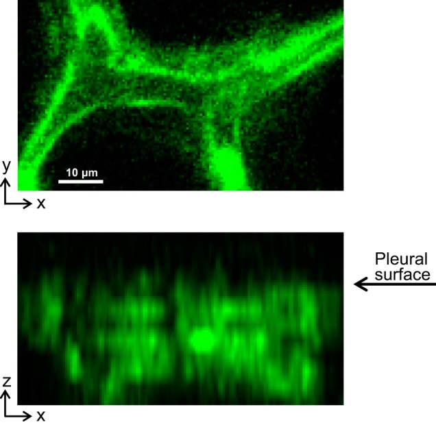
Subpleural septal morphology. Alveoli imaged at P_TP of 4 cmH₂O. Top images show x–y plane of analysis that is parallel to and 22 μm below the pleural surface. Bottom images show x–z sections, with the pleural surface at their tops, constructed from z-stacks of x–y optical sections. The x–z sections intersect the x–y sections along the long axes of the white dotted ovals in the x–y sections. A: subpleural septa are typically oriented perpendicular to the pleural surface. Red arrows show capillary thickness, t_C, of 4.2 μm. B: what look like cross bridges across some alveoli, as viewed in the x–y plane, are arch structures across the tops of the alveoli, as viewed in the x–z plane.

For each septal element at each inflation pressure, we determine strain, e, as:

$$e=\left(L_{\text{Sept}}-L_0\right)/L_0,$$ (1)

where L₀ is the value of L_Sept at P_TP of 0 cmH₂O. With a pixel length of ≤0.36 μm, we can detect a 2-μm change in length (15). We limit our analysis to elements for which L₀ exceeds 20 μm, such that we can detect a strain of 10%.

Experimental/computational determination of septal stress.

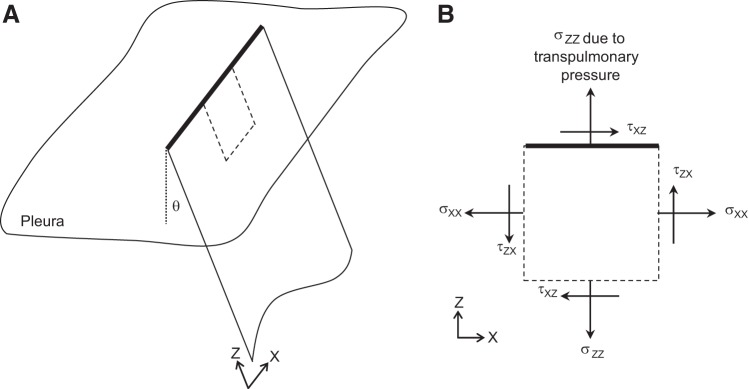
According to Mead et al. (12), P_TP is transmitted to an interior lung region by the septa attached to the periphery of the region and radiating away from the region (Fig. 4A). To determine septal stresses, we thus model application of P_TP to the periphery (Fig. 2, red border; Fig. 4, heavy line) of the analyzed region (Fig. 4B). Given that we determine strains in an x–y optical section that has a z-thickness, h, of 3.5 μm, we determine stresses from forces supported by vertical sections of height h of the imaged septa. Because septal stress is equal to septal force normalized by septal height and thickness, however, the height parameter h cancels from our analysis below. The h value that we use is arbitrary.

Fig. 4.

Modeling P_TP application to the periphery of the analyzed interior lung region. Heavy line indicates periphery of analyzed lung region. A: according to Mead et al. (12), alveolar septa connecting to the outside of an internal lung region and supporting forces F_O transmit P_TP to the interior lung region. Septa within the interior region apply forces F_I to the periphery of the region. B: as forces F_O transmit P_TP to the interior region, we replace them, in our analysis, with application of P_TP directly to the periphery of the interior region. C: for each peripheral element in our linear element model, we calculate the force F_PTP due to pressure acting on the element and apply half of the force at each end point of the element. D: forces acting on peripheral element enclosed by dotted oval in A. Upper left end point is loaded by F_O and also F_P1 from the connecting peripheral element to left. Lower right end point is loaded by F_I and also F_P2 from the connecting peripheral element to right. E: forces acting on peripheral element enclosed by dotted oval in C. Force F_O at upper left end point of the element in D has been replaced by 4 forces due to P_TP, split between both end points (Ei). The 2 forces due to P_TP at each end point may be summed (Eii). Replacement of F_O at 1 end point of the analyzed peripheral element by F_PTP split between its 2 end points reduces loading of the analyzed peripheral element in E compared with that in D.

We calculate the magnitude of the force due to pressure, F_PTP, acting on vertical height h of a given peripheral septal element as

$$F_{\text{PTP}}=P_{\text{TP}}\cdot L_{\text{Sept}}\cdot h.$$ (2)

We specify that F_PTP act perpendicular to and outward from the peripheral septal element within the x–y plane of analysis. Considering each septum as a linear truss element, able to support only axial tension, we apply half of F_PTP at each end point of the element (Fig. 4C).

In applying half of F_PTP at each end point of a peripheral septum, the modeled loading of peripheral septa is less than the actual loading. Actual loading of the peripheral septum in Fig. 4D, due to application of force F_O to its upper left end point by the connecting septum outside of the analyzed region, is greater than the loading of the septum in Fig. 4E, in which case force F_PTP has been split between septal end points. Consequently, we omit peripheral elements when reporting results of our analysis.

At constant P_TP, such as is the case during our image acquisition, the known forces due to pressure acting on the periphery of the analyzed region are at equilibrium with the unknown forces of the strained septal elements of the region. At each node, net forces in the x- and y-directions must equal zero. Thus we generate a system of 2N equations, where N is the number of nodes. With an unknown force in each septal element, we have S unknowns, where S is the number of septal elements. As 2N > S, the system is overdetermined. To solve the system of equations, we generate a vector F_PTP of length 2N containing the x- and y-components of the forces due to pressure that act at the nodes. This vector contains nonzero values for nodes on the periphery of the region and values of zero for internal nodes. To relate F_PTP to the forces within the septal elements, we generate a 2N × S matrix A containing sine and cosine values for the angular orientations of the elements. For example, consider node n that joins septal elements i, j, and k. In F_PTP, element 2n-1 contains the x-component of the force due to pressure that is applied to node n. In matrix A, row 2n−1 contains nonzero terms in columns i, j, and k: cosθ_i, cosθ_j, and cosθ_k, respectively, where θ_i, θ_j, and θ_k are the angles of septal elements i, j, and k with respect to the x-axis. We then solve the equation

$$-{\mathit{F}}_{\mathbf{P}\mathbf{T}\mathbf{P}}=\mathbf{A}{\mathit{F}}_{\mathbf{S}\mathbf{e}\mathbf{p}\mathbf{t}}$$ (3)

by least squares fit in MATLAB (MathWorks, Natick, MA) to determine F_Sept, a vector of length S specifying the internal forces, F_Sept, carried by vertical sections of height h of all septal elements.

To determine the stress, σ, of a given septum from the force F_Sept supported by the septum, we require the septal thickness, t. From measurements of randomly selected septa, we determine the average thickness, t_C, of the fluorescently labeled capillaries within the septa at each P_TP (Fig. 3, Table 1). We then approximate t as t_C + 3 μm, where 3 μm is twice the typical thickness of the blood-gas barrier to each side of the alveolar septal capillary (10). For P_TP > 5 cmH₂O following perfusion arrest, we obtain an average t of ∼6 μm (Table 1) that does not differ from direct septal thickness measurements that we have made, also for P_TP > 5 cmH₂O, in the presence of perfusion (12 ml/min) and fluorescent epithelial labeling (27). In an approximation, we use the same mean t value at a given P_TP as the thickness for all septa at that P_TP. We calculate septal stress as

$$\sigma =F_{\text{Sept}}/\left(th\right).$$ (4)

Table 1.

Septal thickness determined from measurement of capillary thickness

			Inflation				Deflation
PTP, cmH2O:	0	4	6	9	15	25	15	9	6
tC, μm	6.4 ± 1.5*	4.5 ± 0.75†	3.3 ± 0.84‡	3.4 ± 0.84	3.0 ± 0.65	3.0 ± 0.81	2.9 ± 0.61	3.4 ± 0.69	3.6 ± 0.90‡
t, μm	9.4	7.5	6.3	6.4	6.0	6.0	5.9	6.4	6.6

Representative capillary thickness, t_C, determined by measurement of width of fluorescently labeled capillaries in 4 randomly selected septa in each of the 3 imaged areas (n = 12) at each transpulmonary pressure P_TP. Total septal thickness, t, approximated as t_C +3 μm (see text). Statistics, t_C marked by symbol (

^*,

^†, or

^‡) differs from all other t_C lacking same symbol (P < 0.05).

Because F_Sept are the forces supported by vertical sections of height h of the septa, the division of F_Sept by h yields a value of σ that is independent of h. From our x–y plane analysis, we obtain a general relation between septal stress along the x-axis of the x–z plane of the subpleural septum and P_TP. Furthermore, since our x–y plane of analysis is parallel to the pleura, the septal stresses that we determine are principal stresses in the planes of the subpleural septa (appendix).

Estimation of effective Young's modulus.

Using the median septal stress and strain values at each P_TP, we estimate for each of the eight segments into which we divide the ventilation loop the effective incremental Young's modulus of a typical septum. We calculate E_Eff as

$$E_{\text{Eff}}=\left({\overline{\sigma }}_{\text{PH}}-{\overline{\sigma }}_{\text{PL}}\right)/\left({\overline{e}}_{\text{PH}}-{\overline{e}}_{\text{PL}}\right),$$ (5)

where σ̄ and ē are median stress and strain at inflation pressures indicated by subscripts PH and PL, representing the high and low pressure end points for the ventilation segment. For example, E_Eff between P_TP of 9 and 6 cmH₂O on deflation is calculated as E_Eff = (σ̄_9,deflation − σ̄_6,deflation)/(ē_9,deflation − ē_6,deflation). We determine a separate value of E_Eff between the same pressures on inflation. These E_Eff values describe the effective elastic behavior due to tissue elasticity, surface tension, and any alteration in geometry of the typical alveolar septum in situ.

Statistics.

We assess statistical difference between all P_TP groups by ANOVA and post hoc Tukey-Kramer analysis. We make comparisons between data at the same P_TP by Student's t-test. We accept significance at P < 0.05. Unless otherwise specified, results are presented as means ± SD.

RESULTS

We present an analysis of 322 septa from three imaged/analyzed regions, each in a separate lung. Since the system of equations that we solve is overdetermined, residual forces exist at the nodes. Residual node force and, as an indicator of solution accuracy, residual node force normalized by the maximal septal force among the septa attached to a given node, are presented in Table 2.

Table 2.

Group data for residual forces at nodes following least squares solution of Eq. 3 for F_Sept

		Inflation				Deflation
PTP, cmH2O:	4	6	9	15	25	15	9	6
FRes/h, × 10−4 dyn/μm	2.1 ± 1.4	3.2 ± 2.2	4.8 ± 3.4	8.2 ± 5.7	14 ± 10	8.5 ± 6.6	4.8 ± 3.3	3.2 ± 2.2
FRes/FSept,Max	0.21 ± 0.31	0.16 ± 0.17	0.15 ± 0.18	0.15 ± 0.18	0.14 ± 0.19	0.16 ± 0.29	0.14 ± 0.16	0.17 ± 0.22

F_Res, residual force at node; h, vertical (z-axis) height of septal section for which supported forces are determined; F_Sept,Max, maximum of the strained element forces, F_Sept, among the septal elements connected to a given node. Data are for n = 629 nodes from the 3 modeled areas.

Group data for strain and stress at four of the five P_TP along the deflation curve are shown in Fig. 5. Limited septal extension at progressively higher P_TP causes a proportionately greater increase in stress than strain. Data for strain, especially, and stress exhibit marked dispersion (Table 3). Figure 6 shows the spatial variation of strain and stress in one of the analyzed regions. Strain values appear randomly distributed. Stress values appear concentrated around large alveoli (Fig. 6B, *marked) that lack cross bridges (Fig. 2 shows all elements of same region). Quantitatively, stress does not correlate with radial distance from the center of the analyzed region in any analyzed region at any P_TP (R² = 0.04 ± 0.03, n = 24). With increasing P_TP, there is decreased dispersion of the data for the angles between septa meeting at three-way junctions (Table 3). These angles, given the uniform vertical orientation of the subpleural septa through which we image (Fig. 3A), are dihedral angles. The dispersion in dihedral angles is thought to be associated with that in septal stress (14).

Fig. 5.

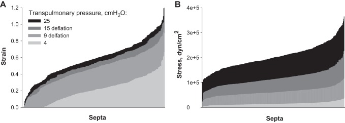
Septal strain and stress. Sorted strain (A) and stress (B) data at 4 P_TP values on deflation. Data presented for n = 322 septa. Peripheral septa, cross bridges, and septa with an unstressed length L₀ < 20 μm are omitted.

Table 3.

Associations of dispersions in data for stress, strain, and dihedral angle with transpulmonary pressure

		Inflation				Deflation
PTP, cmH2O:	4	6	9	15	25	15	9	6
SD of strain/median strain	0.87	0.58	0.47	0.52	0.40	0.56	0.44	0.55
SD of stress/median stress	0.44	0.32	0.29	0.29	0.25	0.28	0.27	0.32
SD of dihedral angles, °	16.2	13.9	12.4	12.2	11.4	11.8	12.1	13.6

P_TP, transpulmonary pressure. Strain and stress data are for n = 322 septa; peripheral septa, cross bridges, and septa with an unstressed length L₀ < 20 μm are omitted. Angle data are for n = 162 3-way septal junctions; junctions connected to peripheral septa, cross bridges, or septa with length L₀ < 20 μm are omitted.

Fig. 6.

Septal strain and stress values in an imaged/modeled lung region at P_TP of 9 cmH₂O on deflation. Peripheral septa, cross bridges, and septa with an unstressed length L₀ < 20 μm are omitted. *Large alveoli lacking cross bridges.

From strain and stress values at each P_TP, we construct a stress-strain curve (Fig. 7). Given the nonlinear nature of the strain and stress distributions, we plot median strain and stress values. Hysteresis is significant at P_TP of 9 and 15 cmH₂O, in agreement with previous reports of hysteresis in whole lung pressure-volume and alveolar surface area-lung volume relations during quasi-static ventilation between FRC and TLC (17, 21). The slope of each segment of the stress-strain curve indicates the effective incremental Young's modulus of an average septum at that degree of lung inflation (Table 4). Along both the inflation and deflation limbs of the ventilation loop, values for E_Eff increase with increasing P_TP. Whereas we determine E_Eff over nearly the full range of physiological lung volumes, E_Eff during tidal breathing would be at the low end of the reported range.

Fig. 7.

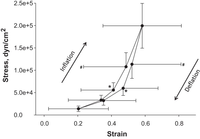
Septal stress-strain relation. Median stress vs. median strain at 8 P_TP around the ventilation loop, for n = 322 septa. Peripheral septa, cross bridges, and septa with an unstressed length L₀ < 20 μm are omitted. Strain and stress both differ significantly (P < 0.05) between the end points of each segment of the stress-strain loop, excepting that there is no difference in strain between P_TP of 25 cmH₂O and 15 cmH₂O on deflation. At P_TP of 9 cmH₂O (*), strain (P < 0.01) and stress (P < 0.01) are greater on deflation than on inflation. At P_TP of 15 cmH₂O (#), strain (P < 0.01) is greater on deflation than on inflation.

Table 4.

Young's modulus values for 8 linearized segments of the ventilation cycle

	Inflation				Deflation
PTP Range, cmH2O:	4–6	6–9	9–15	15–25	15–25	9–15	6–9	4–6
EEff, dyn/cm2	1.4e5	3.1e5	6.9e5	9.5e5	1.4e6	1.0e6	2.4e5	1.2e5
TPL & TPH, dyn/cm	7.2 & 8.6	8.6 & 13.4	13.4 & 20	20 & 30	20 & 30	15 & 20	10.4 & 15	7.2 & 10.4
ETissue, dyn/cm2	1.1e5	1.0e5	4.1e5	6.1e5	8.6e5	7.1e5	1.2e5	6.3e4
ETissue/EEff	0.79	0.33	0.59	0.64	0.61	0.70	0.49	0.51
EBM, dyn/cm2	7.9e6	6.4e6	2.5e7	3.6e7	5.1e7	4.4e7	7.5e6	4.4e6

E_Eff, effective septal Young's modulus, equal to the slope of the relevant segment of the stress-strain curve in Fig. 7 and determined according to Eq. 5; T_PL & T_PH, approximate surface tension values, from Bachofen et al. (1), at the low (PL) and high (PH) pressure end points of the ventilation segment; E_Tissue, Young's modulus of septal tissue, calculated according to Eq. 8; E_BM, Young's modulus of basement membrane, calculated according to Eq. 9.

Cross-bridge elements, which we omit from all analyses above, carry lower stresses than real septal elements at all P_TP. Table 5 displays real septal and cross-bridge stress values.

Table 5.

Stresses in real septal elements and arched cross-bridge structures

	Inflation				Deflation
PTP, cmH2O:	4	6	9	15	25	15	9	6
σReal, dyn/cm2	1.5e4 ± 6.9e3	3.5e4 ± 1.1e4	5.8e4 ± 1.6e4	1.1e5 ± 3.1e4	2.1e5 ± 5.0e4	1.2e5 ± 3.2e4	6.2e4 ± 1.6e4	3.4e4 ± 1.0e4
σCross Bridge, dyn/cm2	1.1e4 ± 5.6e3*	2.3e4 ± 1.2e4*	3.5e4 ± 1.9e4*	5.1e4 ± 3.2e4*	1.1e5 ± 6.3e4*	6.0e4 ± 3.6e4*	3.6e4 ± 1.9e4*	2.2e4 ± 1.1e4*
Mean σCross Bridge/mean σReal	0.70	0.65	0.59	0.45	0.53	0.51	0.57	0.64

σ_Real, Stress supported by real septal elements (n = 322); peripheral septa, cross bridges, and septa with an unstressed length L₀ < 20 μm are omitted. σ_{Cross Bridge}, Stress supported by cross-bridge elements (n = 100); cross bridges with an unstressed length L₀ < 20 μm are omitted.

^*P < 0.01 vs. σ_Real at same P_TP.

DISCUSSION

Inputting in situ data to a model of networked linear elements representing alveolar septa, we determine strain and stress of the elements. From median strain and stress values, we calculate average, effective septal Young's moduli between FRC and near-TLC. To our knowledge, these effective Young's modulus values are the first reported characterization of the mechanical response of in situ septa to lung inflation.

In our investigation of septal mechanics, we perform a linear analysis under static conditions within the physiological range of lung volumes. By ventilating dynamically before pausing for imaging and by partitioning the ventilation cycle into eight segments, we nonetheless detect hysteresis and nonlinear behavior (Fig. 7). Both increasing surface tension and increasing tissue modulus with increasing P_TP no doubt contribute to the nonlinearity, the increase in E_Eff with P_TP. Inflation-induced straightening of any septa that are slack at low P_TP likely contributes to the nonlinearity of the observed stress-strain relation and may result in determined strains that are, especially at low P_TP, greater than true tissue strain. The determined strain, however, underlies alveolar ventilation. Beyond any nonlinear septal geometry evident by light microscopy, pleating of the epithelial basement membrane that is evident by electron microscopy may contribute to septal slackness. As the inflation-induced increase in alveolar septal surface area is essentially the same whether assessed by light or electron microscopy (1), the contribution of unpleating to effective septal mechanics may be limited. Nonetheless, any unpleating that occurs and that contributes to the relative displacement of septal end points is captured in the effective Young's modulus values that we report.

The standard deviation in strain values is essentially independent of median strain value (Fig. 7). The standard deviation in stress, in contrast, increases with median stress value. We interpret the constant strain error to be, principally, a measurement error. In determining strain, we limit our analysis to septal elements with an unstrained length of at least 20 μm to improve our ability to detect small strains. At P_TP of 4 cmH₂O, nonetheless, measured strain is negative for 15% of septa (Fig. 5A, 4 cmH₂O data group does not extend to y-axis). We attribute the finding of negative strain values at low P_TP to the large error in our strain determination method. To determine definitively whether septal strain is ever negative at low P_TP would require a more precise means of length assessment that could be applied in situ in the lung. In the present study with the limited resolution of light microscopy, however, we note that any errors in the placement of nodes at septal junctions should be random such that mean strain values are not affected.

In determining stress, we assume a uniform thickness for all septa. At a given P_TP, we normalize the forces in all septa by the same cross-sectional area. Thus the dispersion in the stress values that we report is directly proportional to the dispersion in forces carried by the elements of our model. Given that t in fact varies between septa and along the length of the individual septum, it is possible that stresses are more uniform than reported. Another contribution to error in stress is the effect of out-of-plane forces applied by arch structures over the tops of subpleural alveoli. We include in our model cross bridges that are evident in the x–y plane of analysis at low inflation pressure. With inflation-induced alveolar expansion in the z-direction, such cross bridges sometimes disappear at high pressure from the morphologically landmarked analysis plane. Yet we retain the cross bridges in our model at all inflation pressures and, in doing so, may underestimate septal stress and effective modulus at high pressure. Despite the variability in reported stress, there is no preferential spatial distribution of stress with respect to radial position in the analyzed area. We interpret the lack of spatial correlation to validate Mead et al.'s model (12), from which we derive our boundary condition.

With our microscopy technique, we are limited to analysis of subpleural alveoli, as has been discussed previously (15). The x–y cross sections that we image through subpleural alveoli (Fig. 2) look typical of randomly oriented sections through the interior of the lung. According to Gil et al. (6) the lung inflation-surface area relation, which is the two-dimensional analog of the one-dimensional lung inflation-septal distension relation characterized in the present study, does not differ between near-surface and internal alveoli. Yet the near-surface alveoli studied by Gil et al. were not subpleural alveoli, as in our own study, and subpleural alveoli do have some distinguishing characteristics. Most strikingly, the alveolar walls that connect to the pleural surface and that we capture in our optical sections tend to be oriented perpendicular to the pleural surface (Fig. 3A) (13). Because of this uniformity of orientation, the stresses that we determine are oriented along principal axes of the alveolar septa. By an alternative measure, subpleural alveoli are less uniform than internal alveoli. The standard deviation in dihedral angles between alveolar septa meeting at three-way junctions in the interior of the lung has been shown to decrease from 6 to 2° with inflation from FRC to TLC; this decrease has been postulated to suggest increased uniformity in septal stress with lung inflation (14). With our ability to determine septal stress, we confirm the association between dispersion in dihedral angles and septal stress. With inflation from P_TP of 4 (FRC) to 25 (nearly TLC) cmH₂O, standard deviation in dihedral angles at three-way intersections of subpleural septa decreases from 16 to 11° and the ratio of standard deviation in subpleural septal stress to median stress decreases from 0.44 to 0.25 (Table 3). The magnitude of the standard deviation in dihedral angles, however, is greater for subpleural than internal septa (14), suggesting that the mechanics of subpleural and internal alveoli may not be identical. One possible reason for the difference in dihedral angle dispersion between subpleural and internal septa is the attachment of subpleural septa to the pleural membrane, which has a modulus about three times that of the septa (9). The extent of the difference between subpleural and internal alveolar mechanics requires further investigation.

Mead et al.'s model (12) describes transmission of the P_TP to an interior lung region by chains of connected septa tethering the interior region to the pleural surface. We apply this model to a group of subpleural alveoli. We note, however, that the imaged alveoli are adjacent to the pleura in only the z-direction that is perpendicular to the pleura. In the x–y plane in which we perform our analysis, the imaged alveoli are internal alveoli, located far from the edge of the lung. In the plane of analysis, as shown in Fig. 2 by the layers of alveoli surrounding the analyzed region, the analyzed region receives the P_TP indirectly, as described by Mead et al., from a pleural surface located beyond the margins of the imaging field (12).

To assess whether the values of E_Eff that we determine are reasonable, we estimate from our results the Young's moduli of the septal tissue, E_Tissue, and of the basement membrane, E_BM. We compare our estimates to previously published values. We note that the total septa stress is

$$\sigma ={\sigma }_{\text{Tissue}}+2\text{T}/t,$$ (6)

where σ_Tissue is septal stress due to tissue stretch, T is surface tension, and the factor 2 in the surface tension term accounts for surface tension acting on both sides of the septum. Given that surface tension is a force per unit length, T is the ratio of the force carried by the interface over a vertical section of height h of the septum to the height h. Dividing T by septal thickness t yields a force per unit area that is the portion of σ that is attributable to surface tension. Combining Eqs. 5 and 6,

$$\begin{gathered} E_{\text{Eff}}=\left({\overline{\sigma }}_{\text{Tissue,PH}}-{\overline{\sigma }}_{\text{Tissue,PL}}\right)/\left({\overline{e}}_{\text{PH}}-{\overline{e}}_{\text{PL}}\right) \\ +2\left({\text{T}}_{\text{PH}}-{\text{T}}_{\text{PL}}\right)/\left[\overline{t}\left({\overline{e}}_{\text{PH}}-{\overline{e}}_{\text{PL}}\right)\right], \end{gathered}$$ (7)

where σ̄_Tissue is median tissue stress and t̄ is the average of the septal thicknesses at the low and high P_TP end points. Solving Eq. 7 for E_Tissue = (σ̄_Tissue,PH − σ̄_Tissue,PL)/(ē_PH − ē_PL), we find

$$E_{\text{Tissue}}=E_{\text{Eff}}-2\left({\text{T}}_{\text{PH}}-{\text{T}}_{\text{PL}}\right)/\left[\overline{t}\left({\overline{e}}_{\text{PH}}-{\overline{e}}_{\text{PL}}\right)\right].$$ (8)

Using surface tension values published by Bachofen et al. (1) and noting that surface tension of the isolated lung is the same in the absence or presence of perfusion (18, 19), we determine E_Tissue and the ratio of E_Tissue to E_Eff (Table 4). Just above FRC, we find E_Tissue to be 1 × 10⁵ dyn/cm² on inflation and 6 × 10⁴ dyn/cm² on deflation, reasonably a little greater than the E_Tissue value of 5 × 10⁴ dyn/cm² found by Cavalcante et al. (2) just above the unstressed state and also greater than an E_Tissue value (converted, by use of a Poisson's ratio of 0.4, from reported shear modulus) of 1.4 × 10⁴ dyn/cm² determined by atomic force microscopy of an unstressed lung slice (8).

We find tissue elastance generally to dominate surface tension (Table 4). Prior studies of the relative contributions of tissue elastance and surface tension have been contradictory. Comparison of air- and saline-inflated lungs on deflation suggests that tissue elastance dominates at low P_TP, surface tension at high P_TP (6). Experimental assessment of basement membrane surface area and theoretical considerations, in contrast, suggest that surface tension dominates at low P_TP on deflation (23, 26). In the present study, after removal of the contribution of surface tension, E_Tissue incorporates the effect of any inflation-induced alteration in septal geometric contour. If, owing to slack septa at low inflation, our reported strain values are greater than true strain, then our reported E_Tissue values are likely lower than true tissue modulus. The degree to which we may underestimate E_Tissue is unknown. Further investigation is required to elucidate the relative contributions of tissue elastance and surface tension.

Given that E_Tissue is a thickness-weighted average of the moduli of tissue components arranged in parallel yet the thin basement membrane has been shown to support essentially all tissue force (24), we can further estimate the Young's modulus of the basement membrane, E_BM, by renormalizing E_Tissue:

$$E_{\text{BM}}=E_{\text{Tissue}}\overline{t}/t_{\text{BM}},$$ (9)

where t_BM is a typical basement membrane thickness of 100 nm (10). Estimated E_BM values range from 4.4 × 10⁶ to 5.1 × 10⁷ dyn/cm² (Table 4), at the high end of or just above the Young's modulus range reported for elastin, 2 × 10⁶ to 1 × 10⁷ dyn/cm² (5, 7, 20), well below that for collagen, 1 × 10⁹ to 3 × 10¹⁰ dyn/cm² (5, 7, 22), and coincident with that for directly tested basement membranes, 2 × 10⁶ to 3 × 10⁷ dyn/cm² (24). As the basement membrane is a heterogeneous, porous structure, both our estimated E_BM values and directly determined E_BM values (24) are effective values, lower than the modulus of the stiffest basement membrane component, collagen.

Our elastic element model shares similarities with other models of lung tissue (2, 11, 25) and of the cellular cytoskeleton (3). However, in previous models moduli were known/assumed and node locations, initially distributed uniformly, were unknown. The situation is reversed in our model. Here, node locations are known, such that actual alveolar geometry in the plane of analysis is an input to our model, but moduli are not. In this scenario, the system is overdetermined and solved by least squares regression. That residual node forces are not zero may be attributed to factors that include the approximation of septa with nonuniform geometries and material properties as simple linear elements, the imperfect incorporation into our modeling of out-of-plane forces applied by cross bridges, and the limited resolution of the light microscopy that we use to determine septal lengths.

A more accurate determination of effective Young's modulus awaits a means of direct in situ septal force determination. Here, with a novel approach, we present estimates of the effective Young's moduli governing in situ alveolar septal mechanics.

GRANTS

This research was supported by American Heart Association grant 09SDG2010097.

DISCLOSURES

No conflicts of interest, financial or otherwise, are declared by the author(s).

AUTHOR CONTRIBUTIONS

C.E.P. conception and design of research; C.E.P. and Y.W. analyzed data; C.E.P. and Y.W. interpreted results of experiments; C.E.P. and Y.W. prepared figures; C.E.P. drafted manuscript; C.E.P. and Y.W. edited and revised manuscript; C.E.P. and Y.W. approved final version of manuscript; Y.W. performed experiments.

Appendix

Determined stresses are principal stresses.

Stress orientation within the subpleural septa that we image is governed by the geometry of the intersection of subpleural septa with the pleural surface. Whether imaging with (Fig. 3) or without (Fig. A1) a coverslip (27), we find the intersection between subpleural septa and the pleural surface to be a straight line. This line (Fig. A2, heavy line) at the intersection of two elastic membranes has the properties of a linear elastic element. Under static conditions, such as those during which we image the lung, tension must be spatially uniform along the line of septal/pleural intersection. Thus, considering a small section at the top of the septum (Fig. A2, right) and regardless of subpleural septal angle θ with respect to the pleural surface, there can be no shear stress along the top of the section/septum. In particular, shear stress τ_xz must be zero along the top and bottom of the section. In order for there not to be a net moment applied to the section, the reaction shear couple τ_zx must also be zero. Without any shear stresses acting on the element, the normal stresses σ_xx and σ_zz, the latter generated by P_TP application across the pleural surface, must be the principal stresses acting on the planar subpleural septum. Imaging parallel to the pleural surface, the stresses that we determine are the principal stresses σ_xx.

Fig. A1.

A subpleural septum imaged in a perfused (12 ml/min) lung without use of a coverslip at P_TP of 15 cmH₂O. Top: x–y section through septum. Bottom: x–z section shows linear border at top of septum where septum intersects with pleural surface. Fluorescence is dye calcein AM loaded into alveolar epithelium.

Fig. A2.

Stresses determined in x–y analysis plane are principal stresses. Left: schematic of planar subpleural septum and its linear junction with the pleural surface. Although subpleural septa typically meet the pleural surface at an angle, θ, of 90°, analysis (see appendix text) is not restricted to any particular θ value. Right: detail of portion of subpleural septum enclosed by dotted line on left. Normal (σ) and shear (τ) stresses act on each edge of the section, with normal stress σ_zz on the top edge attributable to application of the P_TP to the pleural surface. Because the top edge cannot support a shear stress (see text), all shear stresses are zero and normal stresses σ_xx and σ_zz are principal stresses. The x–y plane of our stress-strain analysis is aligned the axis of the principal stress σ_xx.

REFERENCES

- 1.Bachofen H, Schürch S, Urbinelli M, Weibel ER. Relations among alveolar surface tension, surface area, volume, and recoil pressure. J Appl Physiol 62: 1878–1887, 1987 [DOI] [PubMed] [Google Scholar]
- 2.Cavalcante FSA, Ito S, Brewer K, Sakai H, Alencar AM, Almeida MP, Andrade JS, Jr, Majumdar A, Ingenito EP, Suki B. Mechanical interactions between collagen and proteoglycans: implications for the stability of lung tissue. J Appl Physiol 98: 672–679, 2005 [DOI] [PubMed] [Google Scholar]
- 3.Coughlin MF, Stamenović D. A prestressed cable network model of the adherent cell cytoskeleton. Biophys J 84: 1328–1336, 2003 [DOI] [PMC free article] [PubMed] [Google Scholar]
- 4.Fukaya H, Martin CJ, Young AC, Katsura S. Mechanical properties of alveolar walls. J Appl Physiol 25: 689–695, 1968 [DOI] [PubMed] [Google Scholar]
- 5.Fung YC. Biomechanics: Mechanical Properties of Living Tissues (2nd ed.) New York: Springer-Verlag, 1993 [Google Scholar]
- 6.Gil J, Bachofen H, Gehr P, Weibel ER. Alveolar volume-surface area relation in air- and saline-filled lungs fixed by vascular perfusion. J Appl Physiol 47: 990–1001, 1979 [DOI] [PubMed] [Google Scholar]
- 7.Gosline J, Lillie M, Carrington E, Guerette P, Ortlepp C, Savage K. Elastic proteins: biological roles and mechanical properties. Philos Trans R Soc Lond B Biol Sci 357: 121–132, 2002 [DOI] [PMC free article] [PubMed] [Google Scholar]
- 8.Liu F, Tschumperlin DJ. Micro-mechanical characterization of lung tissue using atomic force microscopy. J Vis Exp 54: e2911, 2011 [DOI] [PMC free article] [PubMed] [Google Scholar]
- 9.Luque T, Melo E, Garreta E, Cortiella J, Nichols J, Farré R, Navajas D. Local micromechanical properties of decellularized lung scaffolds measured with atomic force microscopy. Acta Biomater 9: 6852–6859, 2013 [DOI] [PubMed] [Google Scholar]
- 10.Maina JN, West JB. Thin and strong! The bioengineering dilemma in the structural and functional design of the blood-gas barrier. Physiol Rev 85: 811–844, 2005 [DOI] [PubMed] [Google Scholar]
- 11.Maksym GN, Fredberg JJ, Bates JH. Force heterogeneity in a two-dimensional network model of lung tissue elasticity. J Appl Physiol 85: 1223–1229, 1998 [DOI] [PubMed] [Google Scholar]
- 12.Mead J, Takishima T, Leith D. Stress distribution in lungs: a model of pulmonary elasticity. J Appl Physiol 28: 596–608, 1970 [DOI] [PubMed] [Google Scholar]
- 13.Nieman GF, Bredenberg CE, Clark WR, West NR. Alveolar function following surfactant deactivation. J Appl Physiol 51: 895–904, 1981 [DOI] [PubMed] [Google Scholar]
- 14.Oldmixon EH, Butler JP, Hoppin FG., Jr Dihedral angles between alveolar septa. J Appl Physiol 64: 299–307, 1988 [DOI] [PubMed] [Google Scholar]
- 15.Perlman CE, Bhattacharya J. Alveolar expansion imaged by optical sectioning microscopy. J Appl Physiol 103: 1037–1044, 2007 [DOI] [PubMed] [Google Scholar]
- 16.Reifenrath R. The significance of alveolar geometry and surface tension in the respiratory mechanics of the lung. Respir Physiol 24: 115–137, 1975 [DOI] [PubMed] [Google Scholar]
- 17.Robatto FM, Romero PV, Fredberg JJ, Ludwig MS. Contribution of quasi-static tissue hysteresis to the dynamic alveolar pressure-volume loop. J Appl Physiol 70: 708–714, 1991 [DOI] [PubMed] [Google Scholar]
- 18.Schurch S, Bachofen H, Weibel ER. Alveolar surface tension in excised rabbit lungs: effect of temperature. Respir Physiol 62: 31–45, 1985 [DOI] [PubMed] [Google Scholar]
- 19.Schürch S, Goerke J, Clements JA. Direct determination of surface tension in the lung. Proc Natl Acad Sci USA 73: 4698–4702, 1976 [DOI] [PMC free article] [PubMed] [Google Scholar]
- 20.Sherebrin MH, Song SH, Roach MR. Mechanical anisotropy of purified elastin from the thoracic aorta of dog and sheep. Can J Physiol Pharmacol 61: 539–545, 1983 [DOI] [PubMed] [Google Scholar]
- 21.Suzuki S, Akahori T, Miyazawa N, Numata M, Okubo T, Butler JP. Alveolar surface area-to-lung volume ratio in oleic acid-induced pulmonary edema. J Appl Physiol 80: 742–746, 1996 [DOI] [PubMed] [Google Scholar]
- 22.Svensson RB, Hansen P, Hassenkam T, Haraldsson BT, Aagaard P, Kovanen V, Krogsgaard M, Kjaer M, Magnusson SP. Mechanical properties of human patellar tendon at the hierarchical levels of tendon and fibril. J Appl Physiol 112: 419–426, 2012 [DOI] [PubMed] [Google Scholar]
- 23.Tschumperlin DJ, Margulies SS. Alveolar epithelial surface area-volume relationship in isolated rat lungs. J Appl Physiol 86: 2026–2033, 1999 [DOI] [PubMed] [Google Scholar]
- 24.Welling LW, Zupka MT, Welling DJ. Mechanical properties of basement membrane. Physiology 10: 30–35, 1995 [Google Scholar]
- 25.Wilson TA. A continuum analysis of a two-dimensional mechanical model of the lung parenchyma. J Appl Physiol 33: 472–478, 1972 [DOI] [PubMed] [Google Scholar]
- 26.Wilson TA, Bachofen H. A model for mechanical structure of the alveolar duct. J Appl Physiol 52: 1064–1070, 1982 [DOI] [PubMed] [Google Scholar]
- 27.Wu Y, Perlman CE. In situ methods for assessing alveolar mechanics. J Appl Physiol 112: 519–526, 2012 [DOI] [PubMed] [Google Scholar]