

Abstract
The use of alternating electric fields has been recently proposed for the treatment of recurrent glioblastoma. In order to predict the electric field distribution in the brain during the application of such tumor treating fields (TTF), we constructed a realistic head model from MRI data and placed transducer arrays on the scalp to mimic an FDA-approved medical device. Values for the tissue dielectric properties were taken from the literature; values for the device parameters were obtained from the manufacturer. The finite element method was used to calculate the electric field distribution in the brain. We also included a “virtual lesion” in the model to simulate the presence of an idealized tumor. The calculated electric field in the brain varied mostly between 0.5 and 2.0 V/cm and exceeded 1.0 V/cm in 60% of the total brain volume. Regions of local field enhancement occurred near interfaces between tissues with different conductivities wherever the electric field was perpendicular to those interfaces. These increases were strongest near the ventricles but were also present outside the tumor’s necrotic core and in some parts of the gray matter-white matter interface. The electric field values predicted in this model brain are in reasonably good agreement with those that have been shown to reduce cancer cell proliferation in vitro. The electric field distribution is highly non-uniform and depends on tissue geometry and dielectric properties. This could explain some of the variability in treatment outcomes. The proposed modeling framework could be used to better understand the physical basis of TTF efficacy through retrospective analysis and to improve TTF treatment planning.
Keywords: electric field, tumor treating fields, glioblastoma, finite element method
INTRODUCTION
Glioblastoma Multiforme (GBM) is the most common and devastating form of malignant primary brain tumor. Despite recent improvements in the standard of care, which currently consists of surgery followed by radiotherapy plus concomitant and adjuvant chemotherapy with temozolomide (Becker and Yu, 2012), GBM is currently incurable, with a median survival period of 14.6 months (Stupp et al., 2005).
A new therapeutic technology was proposed within the last decade to treat gliomas, particularly GBM. This method is based on the finding that impressed alternating electric fields selectively arrest the growth of cancerous cells, primarily by interfering with mitosis and cytokinesis. The use of these “Tumor Treating Fields” (TTF) is described in several articles (Kirson et al., 2004, Kirson et al., 2007, Kirson et al., 2009a, Kirson et al., 2009b). Specifically, it was reported that by applying electric fields with an optimal frequency of 200 kHz and amplitudes in the range of 1–3 V/cm, the growth of GBM cells in culture could be disrupted (Kirson et al., 2007). The mechanisms of action of TTF are thought to result from the interaction between the applied electric field and polar molecules within the dividing cell that would lead to: 1) disruption of the microtubule spindle formation during the mitotic phase, and 2) motion of polar macromolecules and organelles towards the cleavage furrow during cytokinesis due to dielectrophoresis (Stupp et al., 2012). In vitro experiments also showed that quiescent cells remained morphologically and functionally intact after TTF treatment (Kirson et al., 2004). Because GBM cells divide rapidly while other brain cells divide infrequently, the rationale of using TTFs is that they could potentially target GBM cells selectively while leaving normal brain cells relatively unaffected. This selectivity is a promising advantage of TTFs over other forms of tumor treatment such as radiotherapy or RF ablation.
A medical device using this mechanism of action was approved by the US Food and Drug Administration (FDA) for use in patients with recurrent GBM, following the completion of a Phase III trial (Stupp et al., 2012). This trial concluded that “No improvement in overall survival was demonstrated, however efficacy and activity with this chemotherapy-free treatment device appears comparable to chemotherapy regimens that are commonly used for recurrent glioblastoma. Toxicity and quality of life clearly favoured TTF”. More recently, the FDA authorized a much larger and comprehensive Phase III trial to test the safety and efficacy of this TTF-producing device as an adjuvant to the best standard of care in the treatment of newly diagnosed GBM patients (NCT00916409). The estimated study completion date is April 2015.
To date, however, there have been no physics-based models to predict the electric field and current distributions in the scalp, skull, cerebrospinal fluid, and brain parenchyma produced by a TTF-generating medical device. Such a modeling framework is clearly needed. By predicting the distribution of current and electric fields produced in the brain, we might develop a better understanding of when and why the TTF delivery method may have been effective in the past, and when and why it may not have been. It might also give us the understanding to personalize the treatment, i.e., to predict better how the device would function in individual subjects. This framework might also provide better exclusion criteria and a new methodology for optimizing the delivery of TTFs. The field distribution at the tissue level can also be used to inform subsequent models of the effect of the TTFs on cell division (Kirson et al., 2004).
In this work, we build on our previous experience modeling static and low frequency electric fields used for transcranial brain stimulation (Miranda et al., 2006, Salvador et al., 2011, Miranda et al., 2013b, Merlet et al., 2013) to investigate the intermediate frequency regime used in TTF-based therapy (100–300 kHz). We report the salient features of the electric field distribution in a realistic head model computed using a Finite Element Method (FEM) model and discuss the significance of our findings for improving the application of TTFs. Some data in this study were presented at the 21st Annual ISMRM Meeting, Salt Lake City, USA, April 2013 (Miranda et al., 2013a).
MATERIALS AND METHODS
The spatial distribution of the electric field in the brain was computed using a realistic head model that was created from MRI data. Images were segmented into five different tissue types: scalp, skull, cerebrospinal fluid (CSF), gray matter (GM), and white matter (WM), as described elsewhere (Miranda et al., 2013b). Two pairs of multi-transducer arrays were placed on the scalp. One pair was placed over the left and right temporal and parietal areas (Left-Right or LR arrays), and the other pair was placed over the supraorbital region and at the back of the head (Anterior-Posterior or AP arrays), as shown in Figure 1. Each array consisted of 3×3 interconnected transducers, capacitively coupled to the scalp. Transducers were ceramic disks with 1 mm height and 9 mm radius, and a metal-coated upper surface (the one not in contact with the scalp). The separation between transducer centers was 22 mm in one direction and 33 mm in the other. This accurately represents the geometry of the arrays supplied with the NovoTTF system (http://www.novocure.com) (private communication, E. Kirson, Novocure, July 2012). A thin layer of conductive gel, 0.5 to 2 mm thick and 10 mm in radius, filled the gap between the transducers and the scalp. A volume mesh was then generated and used to calculate the electric field. This FEM modeling framework was based on the following programs: Brainsuite for image segmentation, Mimics for mesh generation and COMSOL for FEM analysis (http://neuroimage.usc.edu/neuro/BrainSuite, http://biomedical.materialise.com/mimics, http://www.comsol.com).
Figure 1.
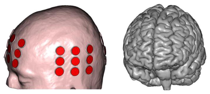
Realistically shaped head model with the left and anterior transducer arrays clearly visible. The representation of the cortical surface illustrates the level of anatomical detail in the model.
The electric field calculations were performed for two different transducer array configurations: LR arrays active and AP arrays inactive (LR configuration), and AP arrays active and LR arrays inactive (AP configuration). In both cases, the frequency of the impressed current was set to 200 kHz, and its amplitude was set to 100 mA at each active transducer (200 mA peak-to-peak).
The tissues were assumed to be isotropic and the values for the electrical conductivity (σ) and relative permittivity (εr) at 200 kHz were estimated from the literature: scalp (Gabriel et al., 1996, Hemingway and McClendon, 1932, Yamamoto and Yamamoto, 1976, Burger and van Milaan, 1943), skull (de Mercato and Garcia Sanchez, 1992, Kosterich et al., 1983, Reddy and Saha, 1984, Law, 1993), CSF (Gabriel et al., 1996, Baumann et al., 1997, Crile et al., 1922), GM and WM (Logothetis et al., 2007, Ranck, 1963, Gabriel et al., 2009, Latikka et al., 2001, Stoy et al., 1982, Surowiec et al., 1986, Van Harreveld et al., 1963, Freygang and Landau, 1955), and tumor (Peloso et al., 1984, Surowiec et al., 1988, Lu et al., 1992, Latikka et al., 2001). These studies report a variety of values for each tissue type. Typical values were chosen for this study and are listed in Table 1. The values for the gel and transducer materials were obtained from the Novocure company.
Table 1.
Values of the electric properties of tissues and other materials at 200 kHz used in this study.
| Dielectric properties | Scalp | Skull | CSF | GM | WM | Virtual lesion | Gel | Transducers | |
|---|---|---|---|---|---|---|---|---|---|
| Tumor | Core | ||||||||
| σ (S/m) | 0.25 | 0.013 | 1.79 | 0.25 | 0.12 | 0.24 | 1.0 | 0.10 | 0 |
| εr | 10000 | 200 | 110 | 3000 | 2000 | 2000 | 110 | 100 | 10000 |
To study the effect of a tumor on the resulting electric field a “virtual lesion” was incorporated in the normal head model. The lesion consisted of two concentric spheres placed in the WM near a lateral ventricle, representing a necrotic core surrounded by a 3mm-thick shell of active tumor. The diameters of the inner and outer spheres were 1.4 cm and 2.0 cm, respectively.
The electromagnetic wavelength in the different tissue types is much larger than the size of the head (15–150 m vs 0.2 m) and so the electro-quasistatic approximation of Maxwell’s equations applies (Haus and Melcher, 1989). COMSOL was used to compute a time-harmonic solution to Laplace’s equation for the electric potential under this approximation and subject to the following boundary conditions: continuity of the normal component of the current density at internal boundaries, zero normal component of the current density at the outer boundary (scalp) and uniform potential on the upper surface of each active transducer subject to the constraint that the integral of the normal component of the current density be equal to a preset value (100 mA).
The current density calculated using this model includes resistive and capacitive components, and the magnitude of the electric field reported here reflects this. However, for the parameters used in this model the current in the head is mainly resistive, i.e., σ ≫ ωεrε0, where ω is the angular frequency, and ε0 is the permittivity of vacuum (Plonsey and Heppner, 1967). Thus, the effect of differences in dielectric properties will be discussed mainly in terms of differences in tissue electrical conductivity.
RESULTS
The spatial distribution of the electric field produced in the normal head model by the TTF arrays is illustrated in Figure 2. The plots on the left and the right columns correspond to the LR and the AP configurations, respectively. On the top row, the magnitude of the field in the GM and WM is shown in an axial slice at the level of the lateral ventricles. The arrows indicate the direction of the alternating field. In both configurations, the magnitude of the electric field exceeded 1 V/cm over large areas of the brain. The field is slightly higher in the LR than in the AP configuration, in the regions close to the ventricles. On the other hand, the field is slightly more uniform in the AP configuration, partly because the effect of the ventricles is less marked and partly because the arrays cover a larger part of the cross-section of the brain seen along the AP direction.
Figure 2.

The electric field magnitude, in V/cm, in the same axial, sagittal and coronal slices for the LR array configuration (left column) and for the AP array configuration (right column). The arrows in the axial plots show the direction of the alternating electric field. Values greater than 3.0 V/cm are shown in dark red.
The plots in the second and third rows of figure 2 show the electric field distribution in sagittal and coronal slices. The electric field also exceeded 1 V/cm over a large part of the brain in the inferior-superior direction, due to the large dimensions of the arrays (about 6.2 cm by 8.4 cm). Nonetheless, the field intensity is lower in slices below and above the arrays. The percentages of the total volumes of WM, GM, and brain (i.e., GM+WM) in which the electric field exceeded 0.5, 1.0, 1.5, 2.0 and 2.5 V/cm are shown in Figure 3, for the two configurations. The graph in the bottom right shows the percentage of the volume of the brain where the electric field exceeded a certain value in both configurations (LR*AP) or in either configuration (LR+LP).
Figure 3.

Percentage of the total volume of a given tissue where the electric field magnitude exceeded the value in the horizontal axis, in V/cm.
The electric field shown in figure 2 is highly non-uniform. This is due to differences in the dielectric properties of the various tissues and to the complex shape of the interfaces separating them, as noted in previous works (Miranda et al., 2007, Miranda et al., 2013b). For example, the magnitude of the electric field is lower in GM than in WM because its conductivity is higher than that of WM. Also, near interfaces that are perpendicular to the applied electric field, the field is increased in the low conductivity tissue and decreased in the high conductivity region. This directional effect is clearly visible in the vicinity of the lateral ventricles, where the high conductivity of the CSF leads to an increase in the electric field in the surrounding brain tissue. It is also present at WM-GM interfaces with the appropriate orientation relative to the applied electric field. In this case, the effect is smaller because the ratio of the conductivities of the two tissues is closer to 1. The increase in the electric field in the WM is more evident closer to the arrays. We will refer to the regions of local field enhancement in the brain as “hotspots”. The term is related to the color scale and not to temperature. No significant temperature increase is expected in the brain due to heat dissipation in the tissue.
The effect of a virtual tumor on the local electric field distribution is illustrated in Figure 4. The field is very low in the necrotic core due to its high conductivity. In the tumor shell, where the conductivity is twice that of WM, the average electric field is lower than in the corresponding region of the contralateral hemisphere. However, directional effects come into play here, too, and the field in the shell is far from uniform: in both configurations, it is increased in the vicinity of the two “poles” where the applied electric field is perpendicular to the spherical surface, and it is reduced around the “equator”. The effect is more pronounced in the LR configuration due to the higher electric field it produces at the location of the tumor.
Figure 4.
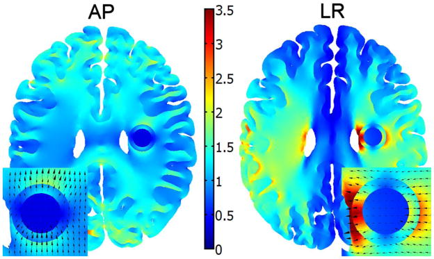
The effect of a tumor with a necrotic core on the magnitude of the electric field, for the AP arrays (left) and LR arrays (right). The direction of the electric field in and around the tumor is shown in the insets. Values greater than 3.5 V/cm are shown in dark red.
We also calculated average electric field values and specific absorption rates (SAR) in the scalp and skull under the transducer arrays. The average electric field values under all transducer arrays were 5.1 V/cm in the scalp and 31 V/cm in the skull, respectively. The corresponding SAR values were 81 W/kg and 77 W/kg. The average SAR in the part of the brain contained in the two cuboid regions defined by the AP and by the LR transducer array pairs was 1.6 W/kg.
DISCUSSION
We have developed a framework to predict the magnitude of the electric field generated in a normal brain by the only device approved for the treatment of recurrent GBM, based on a realistic head model derived from MRI data. For typical impressed current amplitudes we found that the electric field in most of the brain varied between 0.5 and 2.0 V/cm and that it exceeded 1 V/cm in 60% of the brain volume, in either of the two array configurations (Figures 2, 3). Since the efficacy of TTF increases with the number of field directions to which the tumor is exposed (Kirson et al., 2007), we also calculated that 40% of the brain is exposed to an electric field greater than 1 V/cm in both array configurations (AP*LR, Figure 3). It should be noted that there is some uncertainty in the electric properties used in this study, which could affect the calculated electric field values. Nonetheless, there is a reasonable agreement between the values reported here and those that have been shown to slow down cancer cell proliferation in vitro (1–3 V/cm) (Kirson et al., 2007). On the other hand, it is possible that the electric field value required to achieve complete proliferation arrest in glioma cells following a 24 h exposure to TTFields, 2.25 V/cm (Kirson et al., 2004), may only be achieved in limited and specific regions of the brain.
As a result of tissue heterogeneity, the electric field in the brain does not decrease smoothly with distance from the transducers, as it would in a homogeneous tissue. Also, electric field hotspots can occur far from the arrays, giving rise to a complex spatial distribution (Figure 2). This non-uniformity of the electric field could lead to different treatment outcomes depending on the position of the tumor relative to different tissue interfaces, and to the transducers. For example, tumors close to the ventricles may be exposed to higher electric fields, as will superficial tumors close to a transducer.
The existence of electric field hotspots is due to a secondary electric field generated by charge accumulation at tissue interfaces. For purely resistive tissues, the secondary field depends only on the ratio of the conductivities of the two adjacent tissues, and is proportional to the strength of the normal component of the applied electric field (Miranda et al., 2007). Thus, for a given tissue geometry, the intensity of the secondary electric field relative to that of the applied electric field, i.e., the pattern of hotspots, depends only on the relative values of the conductivity, not the absolute values. Published data consistently shows that the conductivity of CSF is at least 4 to 6 time higher than that of GM and WM. Thus the prediction of the existence of hotspots at WM-CSF and GM-CSF interfaces is a robust one. It is also generally accepted that the mean conductivity of WM is lower than that of GM, by a factor of about 2. However, WM is anisotropic as its conductivity depends on fiber orientation. This is expected to affect the distribution of hotspots near the GM-WM interface, as well as the field distribution throughout the WM. In the future we plan to include the anisotropic conductivity of WM in our model. The anisotropic conductivity tensor of WM may be inferred from diffusion tensor MRI (DTI) data, mapped onto the corresponding realistic head model and used in the FEM calculation (Basser et al., 1994, Tuch et al., 2001, Wolters et al., 2006, Hallez et al., 2008, Gullmar et al., 2010). We will also perform a sensitivity analysis using an anisotropic realistic head model, both in terms of the electric conductivity and the thickness of the different tissues.
Tissue heterogeneity is also expected to affect the electric field distribution in the tumor region. Glioblastomas often possess a necrotic core within a high cellularity thick margin that is surrounded by a vasogenic edematous extracellular matrix region (not represented in this model). The core and the edematous regions are likely to have higher conductivities than normal tissue whereas the high cellularity region may have a lower conductivity. The electric field hotspots in the latter region, shown as a thick spherical shell in Figure 4, are due to the higher conductivity attributed to the necrotic core. As at other interfaces, the magnitude of the changes in the electric field depends on the relative values of the conductivities, and directional effects are always present. As a result, the electric field in the tumor is not uniform even when the tumor is subject to a uniform applied electric field. There is little information available regarding the conductivity of tumors at around 200 kHz. In this case, too, the inclusion of DTI-derived conductivity estimates in the model could improve the predictions of the electric field in the tumor region.
In the completed clinical trial, the largest dimension of the tumor treated with TTFs had a median of 6.1 cm and a range of 0–15.2 cm (Stupp et al., 2012). Because the electric field in the brain is not uniform, tumor size will influence the effective electric field over the whole tumor and therefore represents another potential source of variability of the treatment outcome, in addition to tumor location and to heterogeneity effects.
Interestingly, the electric field values reported in this study are similar to or greater than those calculated in transcranial magnetic stimulation (TMS) modeling studies, which are typically around 1 V/cm at threshold (Roth et al., 1991, Salvador et al., 2011). This raises the question why TTFs do not stimulate neurons in the same way as TMS does? The answer lies mainly in the different frequencies employed in the two techniques: 3 kHz for biphasic TMS pulses and 200 kHz for TTFs. Given that the electrical behavior of a passive neural membrane can be described in terms of a parallel RC circuit, the membrane’s response to an applied external electric field varies with frequency. Since the neural membrane time constant is about 100 μs (Barker et al., 1991) or greater, the effect of an alternating electric field on membrane polarization is expected to diminish for frequencies greater than 10 kHz. It is therefore likely that an electric field oscillating at 200 kHz with an amplitude of 1 V/cm is unable to depolarize a neuron to the point of generating an action potential.
The SAR values in the scalp and skull under the transducer arrays are high compared with the 3.2 W/kg limit set by International Standard IEC 60601-2-33 2010 for MR imaging of the head. Despite these high values, effects on the scalp seem to be limited to the mild to moderate contact dermatitis that was observed beneath the transducer arrays in 16% of TTF patients in the clinical trial (Stupp et al., 2012). This limited effect may be due to the power delivered by the TTF device being lowered automatically when the temperature of any transducer exceeded 41°C (Kirson et al., 2007). The high electric field values in the skull could affect hematopoiesis in the cranial marrow. Nonetheless, haematological adverse effects greater than grade 2 only affected 3% of TTF patients in the clinical trial (Stupp et al., 2012), probably because the marrow in other bones was unaffected.
The figures presented in this study and the considerations outlined in this section give a reasonable characterization of the electric field distribution in the brain during a TTF treatment. However, the presence of a tumor, peritumoral edema, and, in some cases, deformed ventricles, is expected to alter this distribution substantially. Patient-specific head models could provide more accurate electric field maps. They could also be used to perform a retrospective analysis of TTF treatments and help explain observed outcomes, both positive and negative. These electric field and other maps could also be used in treatment planning, i.e., to determine a priori the best position of the arrays and the current through individual transducers to optimize electric field delivery to the tumor. For example, one could maximize the electric field strength and uniformity in the tumor and infiltrative edematous territory, and minimize the electric field strength in other areas (Dmochowski et al., 2011, Ruffini et al., 2014). This optimized electric field delivery could also help reduce heat dissipation at the transducer-skin interfaces and the overall power dissipation and/or drainage from the batteries, improving patient comfort and the portability of TTF devices.
CONCLUSION
We predicted for the first time the electric field distribution in the brain during the application of tumor treating fields using a computational modeling framework. The distribution is highly nonuniform and depends on tissue geometry and dielectric properties, which could explain some of the variability in treatment outcomes. The proposed modeling framework can be extended to generate subject-specific models with real brain tumors from structural MRI and DTI data. It could then be used to improve TTF delivery through retrospective analysis and prospective treatment planning.
Acknowledgments
This work was supported by the Foundation for Science and Technology (FCT), Portugal; the Intramural Research Program of the Eunice Kennedy Shriver National Institute of Child Health and Human Development, National Institutes of Health, USA; the Seventh Framework Programme for Research of the European Commission (project HIVE, FET-Open grant 222079).
References
- Barker AT, Garnham CW, Freeston IL. Magnetic nerve stimulation: the effect of waveform on efficiency, determination of neural membrane time constants and the measurement of stimulator output. Electroencephalogr Clin Neurophysiol Suppl. 1991;43:227–37. [PubMed] [Google Scholar]
- Basser PJ, Mattiello J, LeBihan D. MR diffusion tensor spectroscopy and imaging. Biophys J. 1994;66:259–67. doi: 10.1016/S0006-3495(94)80775-1. [DOI] [PMC free article] [PubMed] [Google Scholar]
- Baumann SB, Wozny DR, Kelly SK, Meno FM. The electrical conductivity of human cerebrospinal fluid at body temperature. IEEE Trans Biomed Eng. 1997;44:220–3. doi: 10.1109/10.554770. [DOI] [PubMed] [Google Scholar]
- Becker KP, Yu J. Status quo--standard-of-care medical and radiation therapy for glioblastoma. Cancer J. 2012;18:12–9. doi: 10.1097/PPO.0b013e318244d7eb. [DOI] [PubMed] [Google Scholar]
- Burger HC, van Milaan JB. Measurements of the specific resistance of the human body to direct current. Acta Med Scand. 1943;114:584–607. [Google Scholar]
- Crile GW, Hosmer HR, Rowland AF. The electrical conductivity of animal tissues under normal and pathological conditions. Am J Physiol. 1922;60:59–106. [Google Scholar]
- de Mercato G, Garcia Sanchez FJ. Correlation between low-frequency electric conductivity and permittivity in the diaphysis of bovine femoral bone. IEEE Trans Biomed Eng. 1992;39:523–6. doi: 10.1109/10.135546. [DOI] [PubMed] [Google Scholar]
- Dmochowski JP, Datta A, Bikson M, Su Y, Parra LC. Optimized multi-electrode stimulation increases focality and intensity at target. J Neural Eng. 2011;8:046011. doi: 10.1088/1741-2560/8/4/046011. [DOI] [PubMed] [Google Scholar]
- Freygang WH, Jr, Landau WM. Some relations between resistivity and electrical activity in the cerebral cortex of the cat. J Cell Comp Physiol. 1955;45:377–92. doi: 10.1002/jcp.1030450305. [DOI] [PubMed] [Google Scholar]
- Gabriel C, Peyman A, Grant EH. Electrical conductivity of tissue at frequencies below 1 MHz. Phys Med Biol. 2009;54:4863–78. doi: 10.1088/0031-9155/54/16/002. [DOI] [PubMed] [Google Scholar]
- Gabriel S, Lau RW, Gabriel C. The dielectric properties of biological tissues: III. Parametric models for the dielectric spectrum of tissues. Phys Med Biol. 1996;41:2271–93. doi: 10.1088/0031-9155/41/11/003. [DOI] [PubMed] [Google Scholar]
- Gullmar D, Haueisen J, Reichenbach JR. Influence of anisotropic electrical conductivity in white matter tissue on the EEG/MEG forward and inverse solution. A high-resolution whole head simulation study. Neuroimage. 2010;51:145–63. doi: 10.1016/j.neuroimage.2010.02.014. [DOI] [PubMed] [Google Scholar]
- Hallez H, Vanrumste B, Van Hese P, Delputte S, Lemahieu I. Dipole estimation errors due to differences in modeling anisotropic conductivities in realistic head models for EEG source analysis. Phys Med Biol. 2008;53:1877–94. doi: 10.1088/0031-9155/53/7/005. [DOI] [PubMed] [Google Scholar]
- Haus HA, Melcher JR. Electromagnetic fields and energy. Englewood Cliffs, N.J: Prentice Hall; 1989. [Google Scholar]
- Hemingway A, McClendon JF. The high frequency resistance of human tissue. Am J Physiol. 1932;102:56–9. [Google Scholar]
- Kirson ED, Dbaly V, Tovarys F, Vymazal J, Soustiel JF, Itzhaki A, Mordechovich D, Steinberg-Shapira S, Gurvich Z, Schneiderman R, Wasserman Y, Salzberg M, Ryffel B, Goldsher D, Dekel E, Palti Y. Alternating electric fields arrest cell proliferation in animal tumor models and human brain tumors. Proc Natl Acad Sci U S A. 2007;104:10152–7. doi: 10.1073/pnas.0702916104. [DOI] [PMC free article] [PubMed] [Google Scholar]
- Kirson ED, Giladi M, Gurvich Z, Itzhaki A, Mordechovich D, Schneiderman RS, Wasserman Y, Ryffel B, Goldsher D, Palti Y. Alternating electric fields (TTFields) inhibit metastatic spread of solid tumors to the lungs. Clin Exp Metastasis. 2009a;26:633–40. doi: 10.1007/s10585-009-9262-y. [DOI] [PMC free article] [PubMed] [Google Scholar]
- Kirson ED, Gurvich Z, Schneiderman R, Dekel E, Itzhaki A, Wasserman Y, Schatzberger R, Palti Y. Disruption of cancer cell replication by alternating electric fields. Cancer Res. 2004;64:3288–95. doi: 10.1158/0008-5472.can-04-0083. [DOI] [PubMed] [Google Scholar]
- Kirson ED, Schneiderman RS, Dbaly V, Tovarys F, Vymazal J, Itzhaki A, Mordechovich D, Gurvich Z, Shmueli E, Goldsher D, Wasserman Y, Palti Y. Chemotherapeutic treatment efficacy and sensitivity are increased by adjuvant alternating electric fields (TTFields) BMC Med Phys. 2009b;9:1. doi: 10.1186/1756-6649-9-1. [DOI] [PMC free article] [PubMed] [Google Scholar]
- Kosterich JD, Foster KR, Pollack SR. Dielectric permittivity and electrical conductivity of fluid saturated bone. IEEE Trans Biomed Eng. 1983;30:81–6. doi: 10.1109/tbme.1983.325201. [DOI] [PubMed] [Google Scholar]
- Latikka J, Kuurne T, Eskola H. Conductivity of living intracranial tissues. Phys Med Biol. 2001;46:1611–6. doi: 10.1088/0031-9155/46/6/302. [DOI] [PubMed] [Google Scholar]
- Law SK. Thickness and resistivity variations over the upper surface of the human skull. Brain Topogr. 1993;6:99–109. doi: 10.1007/BF01191074. [DOI] [PubMed] [Google Scholar]
- Logothetis NK, Kayser C, Oeltermann A. In vivo measurement of cortical impedance spectrum in monkeys: implications for signal propagation. Neuron. 2007;55:809–23. doi: 10.1016/j.neuron.2007.07.027. [DOI] [PubMed] [Google Scholar]
- Lu Y, Li B, Xu J, Yu J. Dielectric properties of human glioma and surrounding tissue. Int J Hyperthermia. 1992;8:755–60. doi: 10.3109/02656739209005023. [DOI] [PubMed] [Google Scholar]
- Merlet I, Birot G, Salvador R, Molaee-Ardekani B, Mekonnen A, Soria-Frish A, Ruffini G, Miranda PC, Wendling F. From Oscillatory Transcranial Current Stimulation to Scalp EEG Changes: A Biophysical and Physiological Modeling Study. PLoS ONE. 2013;8:e57330. doi: 10.1371/journal.pone.0057330. [DOI] [PMC free article] [PubMed] [Google Scholar]
- Miranda PC, Correia L, Salvador R, Basser PJ. Tissue heterogeneity as a mechanism for localized neural stimulation by applied electric fields. Phys Med Biol. 2007;52:5603–17. doi: 10.1088/0031-9155/52/18/009. [DOI] [PubMed] [Google Scholar]
- Miranda PC, Lomarev M, Hallett M. Modeling the current distribution during transcranial direct current stimulation. Clin Neurophysiol. 2006;117:1623–9. doi: 10.1016/j.clinph.2006.04.009. [DOI] [PubMed] [Google Scholar]
- Miranda PC, Mekonnen A, Salvador R, Basser PJ. Modeling the electric field distribution within the brain for the treatment of glioblastomas. ISMRM; Salt Lake City, Utah, USA. 2013a. [Google Scholar]
- Miranda PC, Mekonnen A, Salvador R, Ruffini G. The electric field in the cortex during transcranial current stimulation. Neuroimage. 2013b;70:48–58. doi: 10.1016/j.neuroimage.2012.12.034. [DOI] [PubMed] [Google Scholar]
- Peloso R, Tuma DT, Jain RK. Dielectric properties of solid tumors during normothermia and hyperthermia. IEEE Trans Biomed Eng. 1984;31:725–8. doi: 10.1109/TBME.1984.325399. [DOI] [PubMed] [Google Scholar]
- Plonsey R, Heppner DB. Considerations of quasi-stationarity in electrophysiological systems. Bull Math Biophys. 1967;29:657–64. doi: 10.1007/BF02476917. [DOI] [PubMed] [Google Scholar]
- Ranck JB., Jr Specific impedance of rabbit cerebral cortex. Exp Neurol. 1963;7:144–52. doi: 10.1016/s0014-4886(63)80005-9. [DOI] [PubMed] [Google Scholar]
- Reddy GN, Saha S. Electrical and dielectric properties of wet bone as a function of frequency. IEEE Trans Biomed Eng. 1984;31:296–303. doi: 10.1109/TBME.1984.325268. [DOI] [PubMed] [Google Scholar]
- Roth BJ, Saypol JM, Hallett M, Cohen LG. A theoretical calculation of the electric field induced in the cortex during magnetic stimulation. Electroencephalogr Clin Neurophysiol. 1991;81:47–56. doi: 10.1016/0168-5597(91)90103-5. [DOI] [PubMed] [Google Scholar]
- Ruffini G, Fox MD, Ripolles O, Miranda PC, Pascual-Leone A. Optimization of multifocal transcranial current stimulation for weighted cortical pattern targeting from realistic modeling of electric fields. NeuroImage. 2014;89:216–225. doi: 10.1016/j.neuroimage.2013.12.002. [DOI] [PMC free article] [PubMed] [Google Scholar]
- Salvador R, Silva S, Basser PJ, Miranda PC. Determining which mechanisms lead to activation in the motor cortex: A modeling study of transcranial magnetic stimulation using realistic stimulus waveforms and sulcal geometry. Clin Neurophysiol. 2011;122:748–58. doi: 10.1016/j.clinph.2010.09.022. [DOI] [PMC free article] [PubMed] [Google Scholar]
- Stoy RD, Foster KR, Schwan HP. Dielectric properties of mammalian tissues from 0.1 to 100 MHz: a summary of recent data. Phys Med Biol. 1982;27:501–13. doi: 10.1088/0031-9155/27/4/002. [DOI] [PubMed] [Google Scholar]
- Stupp R, Mason WP, van den Bent MJ, Weller M, Fisher B, Taphoorn MJ, Belanger K, Brandes AA, Marosi C, Bogdahn U, Curschmann J, Janzer RC, Ludwin SK, Gorlia T, Allgeier A, Lacombe D, Cairncross JG, Eisenhauer E, Mirimanoff RO. Radiotherapy plus concomitant and adjuvant temozolomide for glioblastoma. N Engl J Med. 2005;352:987–96. doi: 10.1056/NEJMoa043330. [DOI] [PubMed] [Google Scholar]
- Stupp R, Wong ET, Kanner AA, Steinberg D, Engelhard H, Heidecke V, Kirson ED, Taillibert S, Liebermann F, Dbaly V, Ram Z, Villano JL, Rainov N, Weinberg U, Schiff D, Kunschner L, Raizer J, Honnorat J, Sloan A, Malkin M, Landolfi JC, Payer F, Mehdorn M, Weil RJ, Pannullo SC, Westphal M, Smrcka M, Chin L, Kostron H, Hofer S, Bruce J, Cosgrove R, Paleologous N, Palti Y, Gutin PH. NovoTTF-100A versus physician’s choice chemotherapy in recurrent glioblastoma: a randomised phase III trial of a novel treatment modality. Eur J Cancer. 2012;48:2192–202. doi: 10.1016/j.ejca.2012.04.011. [DOI] [PubMed] [Google Scholar]
- Surowiec A, Stuchly SS, Swarup A. Postmortem changes of the dielectric properties of bovine brain tissues at low radiofrequencies. Bioelectromagnetics. 1986;7:31–43. doi: 10.1002/bem.2250070105. [DOI] [PubMed] [Google Scholar]
- Surowiec AJ, Stuchly SS, Barr JB, Swarup A. Dielectric properties of breast carcinoma and the surrounding tissues. IEEE Trans Biomed Eng. 1988;35:257–63. doi: 10.1109/10.1374. [DOI] [PubMed] [Google Scholar]
- Tuch DS, Wedeen VJ, Dale AM, George JS, Belliveau JW. Conductivity tensor mapping of the human brain using diffusion tensor MRI. Proc Natl Acad Sci U S A. 2001;98:11697–11701. doi: 10.1073/pnas.171473898. [DOI] [PMC free article] [PubMed] [Google Scholar]
- Van Harreveld A, Murphy T, Nobel KW. Specific impedance of rabbit’s cortical tissue. Am J Physiol. 1963;205:203–7. doi: 10.1152/ajplegacy.1963.205.1.203. [DOI] [PubMed] [Google Scholar]
- Wolters CH, Anwander A, Tricoche X, Weinstein D, Koch MA, Macleod RS. Influence of tissue conductivity anisotropy on EEG/MEG field and return current computation in a realistic head model: A simulation and visualization study using high-resolution finite element modeling. Neuroimage. 2006;30:813–826. doi: 10.1016/j.neuroimage.2005.10.014. [DOI] [PubMed] [Google Scholar]
- Yamamoto T, Yamamoto Y. Electrical properties of the epidermal stratum corneum. Med Biol Eng. 1976;14:151–8. doi: 10.1007/BF02478741. [DOI] [PubMed] [Google Scholar]