Investigating Population History Using Temporal Genetic Differentiation

Abstract

The rapid advance of sequencing technology, coupled with improvements in molecular methods for obtaining genetic data from ancient sources, holds the promise of producing a wealth of genomic data from time-separated individuals. However, the population-genetic properties of time-structured samples have not been extensively explored. Here, we consider the implications of temporal sampling for analyses of genetic differentiation and use a temporal coalescent framework to show that complex historical events such as size reductions, population replacements, and transient genetic barriers between populations leave a footprint of genetic differentiation that can be traced through history using temporal samples. Our results emphasize explicit consideration of the temporal structure when making inferences and indicate that genomic data from ancient individuals will greatly increase our ability to reconstruct population history.

Introduction

Recent advances in molecular genetics have opened up the possibility of using temporal genetic samples to answer biological questions, including studies focusing on viruses (Rodrigo and Felsenstein 1999) and studies of animal and human remains (Shapiro and Hofreiter 2014). DNA extraction from fossils or ancient material was pioneered some 3 decades ago (Higuchi et al. 1984; Pääbo 1985), but the field of ancient DNA has been plagued by problems such as contamination from modern-day DNA, postmortem DNA damage, and low levels of endogenous DNA. However, many problems have been resolved in the last few years. For example, the high frequency of postmortem damage in ancient DNA sequences (Briggs et al. 2007) can be difficult to distinguish from biological polymorphisms, but experimental solutions have been developed, such as using enzymes to repair damaged nucleotides (Briggs et al. 2010). Likewise, problems arising from contamination from present-day individuals can be circumvented using these same postmortem damage patterns (Krause et al. 2010; Meyer et al. 2014; Skoglund et al. 2014), coupled with an assessment of whether the DNA originates from a single individual (Green et al. 2010; Krause et al. 2010). These advances have resulted in a remarkable development, exemplified by the explosion in genomic studies of ancient hominid remains such as the sequencing of the Neandertal genome (Green et al. 2010; Prufer et al. 2014), the Denisova genome (Reich et al. 2010; Meyer et al. 2012), and genomic investigations of several prehistoric humans (Rasmussen et al. 2010; Keller et al. 2012; Sánchez-Quinto et al. 2012; Skoglund et al. 2012; Raghavan et al. 2014). There are even isolated examples of DNA preservation in fossils that are hundreds of thousands years old (Orlando et al. 2013; Meyer et al. 2014). The new sequencing technologies have been instrumental for this development simply because they work with massive amounts of short-fragmented DNA, which is the state in which we find postmortem DNA.

Theoretical aspects of temporal genetic differentiation have not been extensively investigated even though many of the classical population-genetic parameters, such as Wright’s F-statistics (Wright 1949), stem from temporal models. For example, temporal differences between ancient samples, as well as between ancient samples and modern-day ones, complicate interpretations of population-genetic structure. Even in the absence of population structure, genetic drift is expected to produce genetic differences between genetic data from different points in time (Krimbas and Tsakas 1971; Waples 1989; Nordborg 1998; Anderson et al. 2000; Wang 2001; Berthier et al. 2002; Beaumont 2003; Depaulis et al. 2009; Nyström et al. 2012), which in practice makes separating historical scenarios of replacement and genetic drift difficult (Nordborg 1998; Serre et al. 2004; Haak et al. 2005; Castroviejo-Fisher et al. 2011; Sjödin et al. 2014). However, it may be desirable to use the temporal structure within a sample to make inferences, because time-structured data offer a new dimension of information for learning about the demographic history. That important information can be extracted from temporal samples is illustrated by the long tradition of using variance in allele frequencies between multi-individual samples from discrete time points to infer effective population size (Krimbas and Tsakas 1971; Waples 1989; Anderson et al. 2000; Wang 2001; Berthier et al. 2002; Beaumont 2003) and methods for using single-locus nonrecombining markers, such as mitochondrial DNA, to infer population size changes (Drummond et al. 2005; Ramakrishnan et al. 2005; Chan et al. 2006; Drummond and Rambaut 2007; Ramakrishnan and Hadly 2009; Navascues et al. 2010; Ho and Shapiro 2011). Furthermore, the coalescent model (Kingman 1982) is readily adapted to accommodate time-serial samples (Rodrigo and Felsenstein 1999) and several simulation tools that handle temporal samples have been developed (Anderson et al. 2005; Jakobsson 2009; Excoffier and Foll 2011). However, the use of genomic data from temporal samples for inferring more complex population histories remains largely unexplored. As the quality and quantity of ancient genomic data is increasing, we need a better understanding of how temporal structure affects genetic differentiation and diversity. In this article, we first illustrate how temporal structure relates to classical models of population structure by calculating Wright’s fixation index, F_ST, in simple demographic models, which provides an intuitive understanding of the problem at hand. Second, we demonstrate that genetic data from temporal samples can greatly aid inferences of population history by highlighting several instances where wide temporal sampling can provide insights that would be hard to obtain otherwise.

Fundamental Properties of Temporal Genetic Structure

Genetic drift results in differentiation between structured populations (Wright 1940, 1951). In a coalescent framework (Kingman 1982; Hudson 1990; Slatkin 1991), genetic differentiation between populations can be viewed as the effect of a shorter expected time of coalescence for lineages from the same population E[T_W] compared with the expected time of coalescence for lineages from different populations E[T_B]. A fundamental metric of genetic differentiation in structured populations is Wright’s fixation index F_ST which, in coalescent terms, corresponds to 1−[E[T_W]/((E[T_W] + E[T_B])/2)], where E[T_W] and E[T_B] are averaged across populations and comparisons (Slatkin 1991). Taking mutations into account, this can be expressed in terms of probabilities of identity by descent (IBD) such as F_ST = (f_w − f_b)/(1 − f_b). Here, f_b is the probability of IBD for lineages picked from different populations and f_w is the probability of IBD for lineages picked from the same population (averaged over the different populations). For instance, if f₁ and f₂ are the probabilities of IBD in two different groups 1 and 2

$$F_{\text{ST}}=\frac{0.5\left(f_1+f_2\right)-f_{\text{b}}}{1-f_{\text{b}}}.$$ (1)

In this article, we consider F_ST for models where samples are drawn from two time points and compare this situation to a model where the two samples are drawn from different populations that diverged at some point in the past (fig. 1).

Fig. 1.

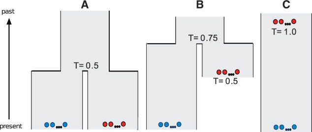
Additivity of genetic drift can result in equivalent genetic differentiation (F_ST) under temporal structure and population divergence. (A and B) Thirty individuals are sampled from two populations (15 individuals from each population) that diverged at a given time in the past. In (A), both samples are taken at the present, and in (B), one of the samples is taken at 0.5 × 2N_e generations before present and the other sample is taken at present. (C) Thirty individuals are sampled from two discrete time points (15 individuals from each time point) in the history of a continuous population. In all three scenarios, the total time that passes between each sample is T = 2N_e generations. The 15 individuals in each sample are illustrated as a series of red circles or a series of blue circles.

If the population size N is constant, the probability of IBD in both the temporal model and the divergence model for lineages picked from the same population is

$$f_1=f_2=\frac{{\left(2N\right)}^{-1}}{{\left(2N\right)}^{-1}+2\mu }=\frac{1}{1+\theta },$$ (2)

where µ is the mutation rate per site per generation and θ = 4Nµ. This is simply the probability that two lineages coalesce before a mutation occurs (2µ is the mutation rate in the two lineages [ignoring µ² terms] and (2N)⁻¹ is the coalescence rate). As for the probability of IBD between populations, in the divergence model (fig. 1A) it is

$$f_{\text{b}}={(1-\mu )}^{t_1}{(1-\mu )}^{t_2}\frac{{\left(2N\right)}^{-1}}{{\left(2N\right)}^{-1}+2\mu }\approx \frac{\text{exp}(-\theta (T_1+T_2)/2)}{1+\theta },$$ (3)

where T₁ = t₁/2N and T₂ = t₂/2N and t₁ and t₂ are the times (in generations) to the split of the two populations. This expression is derived from considering that neither lineage can have a mutation before they reach the ancestral population, and once in the ancestral population, they must coalesce before a mutation occurs (as above). Applying the same argument for the temporal model (fig. 1C), two lineages sampled t generations apart will be IBD if there is no mutation in the younger lineage during t generations and, once in the ancestral population, the two lineages coalesce before any of them mutate. Hence,

$$f_{\text{b}}={(1-\mu )}^t\frac{{\left(2N\right)}^{-1}}{{\left(2N\right)}^{-1}+2\mu }\approx \frac{\text{exp}(-\theta T/2)}{1+\theta },$$ (4)

where T = t/2N. If T = T₁ + T₂ then F_ST in the temporal and divergence model is the same and

$$F_{\text{ST}}=1-\frac{\theta }{\theta +1-\text{exp}\left(-\theta T/2\right)}.$$ (5)

Note that this extends naturally also for models with both divergence and temporal samples, such as the model in figure 1B. However, this simple relationship between temporal structure and divergence models only holds when the population size is constant. When the population size is not constant, F_ST in the temporal and divergence models is expected to be equal only under very specific conditions (see supplementary fig. S1, Supplementary Material online).

Nei’s Estimator of Divergence Time between Populations

Based on a result from Nei (1973), it is commonly stated that expected F_ST in a divergence model with constant size equals 1−e^−T/2 (letting T denote the total time in coalescent units that separates two populations as above). This result was derived under a very specific model assumption—namely that all polymorphisms were present in the ancestral population. Furthermore, this only applies when sampling times are equal, because for a temporal model where polymorphisms were present in the ancestral population, we find instead that F_ST = (1−e^−T)/2 (supplementary material, Supplementary Material online). Curiously, simulations highlight the generality with which F_ST responds to genetic drift under constant-size scenarios, because Nei’s case with ascertainment of polymorphic loci in the ancestral population of the divergence model (F_ST = 1−e^−T/2) corresponds to the temporal case if ascertainment of polymorphisms is performed at the midpoint between the two temporal samples (fig. 2). Likewise, the expectation when polymorphisms are ascertained in the ancestral population of the temporal model (F_ST = (1−e^−T)/2) corresponds to ascertaining in one of the two populations of the divergence model (fig. 2).

Fig. 2.

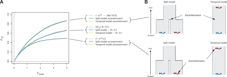
Dependence of F_ST in temporal and divergence models conditioning on the allele being polymorphic. (A) F_ST as a function of T, the total time that separates two populations (two times the population divergence time) or the time that separates two samples in model of samples taken at two different time points. The gray line shows the function F_ST = 1−e^−T/2 (Nei 1973). (B) The models used for simulating population-genetic data and computing F_ST. The split model illustrates a population split T/2 time units in the past and the temporal model that illustrates a single population (of constant size) from which samples have been taken at two time points. Arrows point to where, in time, sites have been ascertained for variation (see main text for a full description of the procedure).

F_ST and the Combined Effect of Migration and Temporal Structure

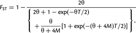
We study the effect of migration by considering a simple island/stepping-stone model with two populations/demes of equal size N and a symmetric migration rate, m, between them and with the two populations being sampled t generations apart. In this case, F_ST can be shown to be

(6)

where θ = 4Nµ, M = 2Nm, and T = t/2N (see supplementary material, Supplementary Material online). As M increases, this expression converges to the formula for F_ST in a pure temporal model with a population of constant but twice as large effective population size (so that the scaled mutation rate is larger by a factor 2, whereas the scaled time is half as large, compare to eq. 5 above). Intuitively, increasing the migration rate lowers F_ST, whereas an increase in time between the sampled time points increases F_ST (fig. 3). Importantly, for a fixed value of F_ST (and θ), there is no definite solution in terms of M because this will depend on T, so that F_ST is not a direct measure of migration rate under this model unless T is known (which requires that N and t are known). This is similar to the difficulty associated with differentiating between population split time and migration in spatial divergence models (Nielsen and Wakeley 2001).

Fig. 3.

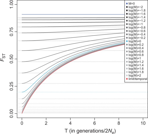
Dependence of F_ST in a simple temporal island model. The model consists of two equally sized populations with symmetric migration rate. The X axis shows the separation in (scaled) time between the samples. θ (the scaled mutation rate) is set to 0.1. The continuous lines show how F_ST for models with different (scaled) migration rates depends on time separation. The dotted lines show F_ST if the samples are not separated in time or, equivalently, if the effective population size is infinitely large. The red line is the limit when migration is infinitely fast. In this case, the model is identical to a purely temporal model with a doubled (and constant) population size (the larger population size implies that θ is twice as large). The dark blue line is the limit when there is no migration while the light blue line at log(M)=0 is included for reference.

Results

The simple theoretical models considered above indicate that both temporal structure and spatial structure affect F_ST in a rather similar manner but that their effects are sufficiently different to prompt caution in interpretations of F_ST, in particular for cases where temporal samples are involved. To investigate more complex scenarios of continuous sampling over time, we now turn to a simulation-based approach.

Stepping-Stone Migration Model with Temporal Samples

In contrast to isolation models, stepping-stone migration models—where populations (demes) are connected in one- or two-dimensional landscapes—typically result in continuous differentiation between individuals rather than discrete genetic clusters of individuals (Novembre and Stephens 2008; Engelhardt and Stephens 2010). Given that temporal genetic structure also affects expected coalescence times between lineages, it can be expected that temporal differentiation would display similar behavior. To demonstrate this phenomenon, we designed a temporal simulation algorithm (see Materials and Methods) based on Hudson’s “ms” coalescence simulation software (Hudson 2002) and simulated a model with 100 demes in a two-dimensional habitat (10 × 10 lattice) with stepping-stone migration. We used 4N_em = 2, where m is the fraction of each subpopulation made up of new migrants each generation (note that scaling in ms is slightly different to the theory above) and sampled one haploid individual from each deme at ten time points separated by t = 4N_e generations, creating a three-dimensional model comprising the two spatial dimensions and the temporal dimension (fig. 4A). Because of the increased complexity of the data, pairwise comparisons such as F_ST are poorly suited to analyze the results. Instead, we used principal component analysis (PCA) to summarize and visualize the resulting population-genetic data (see Materials and Methods). PCA and F_ST have strong conceptual connections, with principal components (PCs) being closely related to the average coalescent times between pairs of haploid genomes (McVean 2009). We find that the first three PCs mirror the three dimensions of the model (three-dimensional Procrustes correlation: 0.984, P < 10⁻⁵) (fig. 4B). Specifically, PC1 and PC2 represented isolation-by-distance in the two-dimensional habitat, whereas PC3 represented temporal differentiation (supplementary fig. S2, Supplementary Material online), but this order of PCs will depend on the relative magnitudes of the scaled migration rate and genetic drift between time points (McVean 2009).

Fig. 4.

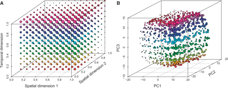
Genetic differentiation mirrors the sampling scheme in a model with both temporal and spatial structure. (A) Two-dimensional stepping-stone migration model from which ten haploid individuals were sampled at different historical time points. (B) PCA of data generated under the model. Large symbols correspond to high PC1 and PC3 values but low PC2 values.

Temporal Genetic Differentiation Can Be Informative about Complex Population Histories

As illustrated in figure 1C, genetic differentiation can also occur in the absence of any spatial structure, that is, in samples taken at different time points from a single continuous (unstructured) population. To investigate temporal differentiation more closely, we simulated a single continuous population with an effective population size of 5,000 diploid individuals and a generation time of 25 years, sampling 20 diploid individuals from the present, and an additional 20 diploid individuals evenly distributed over the period 500–10,000 years ago with a 500-year interval between each sampled individual (fig. 5A). In a PCA, we see that PC1 captures the temporal genetic differentiation, separating the samples from the most recent to the most ancient as a monotonic (but not linear) cline, where individuals close in time are also more genetically similar (fig. 5D and supplementary fig. S3, Supplementary Material online). To investigate the effect of population size fluctuations (i.e., fluctuations in the magnitude of genetic drift), we reduced the population to a tenth of its original size between 5,000 and 5,500 years before present. Under this sampling scheme, the bottleneck is easily detected as a discontinuation in the monotonic cline (fig. 5B and E and supplementary fig. S3, Supplementary Material online).

Fig. 5.

Temporal sampling distinguishes genetic drift from population structure. (A) Constant population size model. (B) Bottleneck model. (C) Replacement model. (D) PC1 stratified by sample time under the constant population size model. (E) PC1 stratified by sample time under the bottleneck model. (F) PC1 stratified by sample time under the replacement model. Each colored circle corresponds to a single-sampled individual except for the large circles at time zero which corresponds to 20 sampled individuals in A, B, and C (in D, E, and F, the 20 individuals sampled at time zero end up on top of each other). F_ST between samples from before and after the bottleneck/replacement events at 5,500 years ago fails to distinguish between the models (F_ST = 0.0154 ± 0.0003 and 0.0153 ± 0.0003, respectively, see fig. 6).

We also simulated population-genetic data under a divergence model of two populations that diverged 10,000 years ago (fig. 5C). Ten ancient individuals were sampled at different time points between 10,000 and 5,500 years from one population, and 30 individuals were sampled from the other population, between 5,000 years ago and the present (ten ancient individuals spread out in time and 20 present-day individuals). This simulation could correspond to a scenario where the older population was replaced with new colonizers from another population. In the simulated data, individuals sampled before the replacement event show a trajectory along PC1 through time that is angled away from the individuals in the population that replaced the previous population (fig. 5F and supplementary fig. S3, Supplementary Material online). In contrast, in the bottleneck scenario, the sampled individuals from before the bottleneck event show a trajectory along PC1 as a function of time that is angled toward the individuals in the descendant population (fig. 5E and supplementary fig. S3, Supplementary Material online). However, F_ST between the ancient individuals from before and after the event was indistinguishable under the bottleneck model and the replacement model (0.0154 ± 0.0003 and 0.0153 ± 0.0003, respectively; fig. 6). To complement the PCA approach, we reconstructed maximum-likelihood trees (supplementary fig. S4, Supplementary Material online) using the covariance in allele frequencies between individuals (Pickrell and Pritchard 2012) and other pairwise F_ST comparisons (fig. 6). This analysis gave different results depending on the way the samples were obtained. The two scenarios were (again) indistinguishable if the samples were grouped into three separate temporal samples. In contrast, if the full temporal structure was accounted for so that each sample was treated independently, the maximum-likelihood trees revealed a difference between the bottleneck model and the replacement model. These observations illustrates that many inference tools can lead to incorrect conclusions for temporally sampled data, and they emphasize the importance of considering detailed temporal sampling structure for distinguishing between bottleneck and replacement models. It also illustrates that the considerable power to distinguish different models that we report is not directly linked to the use of PCA methods but is mainly due to the temporal sampling schemes.

Fig. 6.

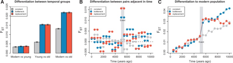
Genetic differentiation between temporal sample groups. (A) F_ST computed on aggregated sample groups is unable to differentiate the bottleneck and replacement models. “Moderns”: 20 samples from time 0. “Young”: 10 samples from time 0–5,000 years ago. “Old”: 10 samples from 5,500 to 10,000 years ago. (B) F_ST between individuals adjacent in time is able to detect a sudden increase in F_ST between the pair of individuals that flank the demographic event (both bottleneck and replacement), but we are unable to separate the replacement and bottleneck scenarios. Standard errors are not shown but ranged between 0.002 and 0.003. (C) F_ST between 20 modern individuals and each ancient individual. Standard errors are not shown but ranged between 0.0010 and 0.0014.

Transient Genetic Barriers

To study more complex population models, we simulated a population split model which involved two populations (A and B) that diverged 8,000 years ago. We kept the same simulation parameters and temporal sampling scheme as above but assigned the 4 ancient individuals from 3,500, 4,500, 5,500, and 6,500 years ago to population B and the remaining 16 ancient individuals to population A (fig. 7A). Strikingly, the population split event is readily identifiable when PC1 is stratified by sampling time (fig. 7C and supplementary fig. S3, Supplementary Material online). In a further modification of the model, we simulated secondary admixture between the two populations 3,000 years before present and where 75% of the genetic material of the recent population was contributed by population A and 25% was contributed by population B (fig. 7B). A plot of PC1 versus sampling time shows the two series of individuals represented by samples from the two populations becoming more similar as time approaches the time of admixture (fig. 7D and supplementary fig. S3, Supplementary Material online), suggesting that transient genetic barriers can be investigated using continuous temporal genetic data.

Fig. 7.

Temporal sampling can be used to detect transient genetic barriers. (A) Split model. (B) Split-admixture model. (C) PC1 stratified by time for data simulated under the split model. (D) PC1 stratified by time for data simulated under the split-admixture model. Each colored circle corresponds to a single sampled individual except for the large circles at time zero, which corresponds to 20 sampled individuals in A and B (in C and D, the 20 individuals sampled at time zero overlap). The 4 ancient individuals from 3,500, 4,500, 5,500, and 6,500 years ago (marked circles) were sampled from population B (bottom population in the model illustrations) and the remaining ancient 16 individuals were sampled from population A (top population in the model illustrations).

Approximate Bayesian Computation Using Temporal Genetic Differentiation

The observation that some statistics of temporal genetic differentiation can recapitulate population history suggests that those statistics can be used to infer population history in more formal settings. We used approximate Bayesian computation (Tavare et al. 1997; Pritchard et al. 1999; Beaumont et al. 2002) to exemplify that temporal genetic data can be used to infer parameters of a demographic model based solely on PC1 loadings of sampled individuals as summary statistics. We applied this approach to a data set consisting of 44 Siberian Woolly Mammoth samples spanning 50,000 years and genotyped at four microsatellites (Nyström et al. 2012). The original study used conventional summary statistics and aggregated temporal groups to show that a population size reduction during the Holocene transition could explain the fact that two temporal groups were genetically differentiated. Here, we expand the inference to a three-parameter model (fig. 8): The time of change, the effective population size before the change, and the effective population size after the change, allowing for either a reduction or expansion in population size (see Materials and Methods). The estimated posterior distribution indicates a size reduction at around 11,200 years ago with the effective population size in the more recent time period being approximately ten times smaller than before the change (table 1 and fig. 8). The inferred timing of this population size reduction coincides with the isolation of Wrangel Island from the Siberian mainland (Vartanyan et al. 1993) and thus corroborates the hypothesis that this restriction of the habitat triggered a founder event in the resident mammoth population (Nyström et al. 2010, 2012).

Fig. 8.

Approximate Bayesian Computation of Woolly Mammoth demographic history using PC1 loadings as summary statistics. (A) Plot of PC1 versus the age of the mammoth individuals. (B) Illustration of the three-parameter model of instantaneous size change. (C) Estimated posterior distribution for the time of size change. (D) Estimated posterior distributions of effective population size before and after the size change. Prior distributions in (C) and (D) are shown by the gray lines.

Table 1.

ABC Inference of Northeast Siberian Woolly Mammoth Demographic History Using PC Loadings as Summary Statistic.

Parameter	Prior (Uniform)	Posterior Mode	Posterior 95% CI
Ne before change	200–50,000	23,500	16,900–29,400
Ne after change	200–50,000	1,800	1,000–8,300
Time of change (years ago)	3,000–40,000	11,200	5,100–23,100

Note.—ABC, approximate Bayesian computation. N_e is the effective population size.

Pitfalls When Comparing Ancient Genomes to Modern Populations

A common situation is that a single ancient genome is available from a certain time point, and the goal is to investigate the historical relationship between the ancient individual and present-day populations. To investigate the differentiation between a single ancient genome and more recent populations, we simulated ten individuals from each of two populations (A and B) which diverged 20,000 years ago (N_e = 10,000) and a single 18,000-year-old individual from the lineage leading to population B (fig. 9). Using PCA, we found that PC1 captures the spatial differentiation between populations A and B, whereas PC2 captures the temporal differentiation between the ancient sample and the modern sample (fig. 9C). The ancient sample appears closer to population B, recapitulating the population history. However, when we modified the model to include a 10-fold population size reduction in population B after the time of sampling of the ancient genome (15,000 years ago; fig. 9B), the ancient sample instead clustered closer to population A (fig. 9D), despite the fact that the ancient individual was sampled from the population that is ancestral to the extant sample from population B. This pattern is due to the fact that less time (on the coalescent scale) has passed between the ancient sample and the extant sample from population A, and the genetic differentiation between the ancient individual and the extant sample from population A (F_ST = 0.030 ± 0.001) was also smaller than the genetic differentiation between the ancient sample and the extant sample from population B (F_ST = 0.055 ± 0.001). Thus, if the demographic history was unknown, one could possibly mistakenly conclude that the ancient sample shares a more recent genetic history with population A, solely due to the different magnitudes of genetic drift. Indeed, the parameter of historical interest is often the degree of shared history, that is, the amount of shared genetic drift and not the relative degrees of differentiation. Accordingly, we were able to identify the correct topology (fig. 9E and F) using concordance tests (Schlebusch et al. 2012; Skoglund et al. 2012) and D statistics (Reich et al. 2009; Durand et al. 2011; Patterson et al. 2012) that are less sensitive to lineage-specific genetic drift.

Fig. 9.

Comparing a single ancient genome to modern populations. (A) Population divergence model with constant effective population size. (B) Population divergence with a 10-fold population size reduction postdating the ancient individual. (C) PCA of 100,000 SNPs simulated under the model in (A). (D) PCA of 100,000 SNPs simulated under the model in (B). (E) Population topology inferred using C tests and D tests based on 100,000 independent SNPs simulated under the model in (A), and (F) population topology inferred using C tests and D tests based on 100,000 independent SNPs simulated under the model in (B). Values for the C-statistic are only positive for the correct topology, and absolute values of the D-statistic are lowest for the correct topology. The tree topologies displayed in (E) and (F) represent the three possible topologies tested and the larger trees represent the true topology (and also the one supported by the statistics). The gray circles in (E) and (F) represent an outgroup individual constructed from the ancestral alleles of each simulated locus. For details on these tests, see Materials and Methods.

Discussion

The main insight that arises from our analyses is that wide temporal sampling provides information that can be hard to attain using modern-day data alone or more clustered temporal groups. The importance of wide temporal sampling could also explain previous results suggesting that not much statistical power is gained solely by adding one or a few temporal sample groups (Mourier et al. 2012). Spatial sampling structure can also have a substantial impact on inferences of population history using modern-day data (Serre and Pääbo 2004; Rosenberg et al. 2005; Chikhi et al. 2010; DeGiorgio and Rosenberg 2013) in which case differentiating between the relative contributions of migration and genetic drift because population divergence is a serious challenge (Nielsen and Wakeley 2001). In contrast to the many similarities between spatial and temporal structure that we have highlighted, the possibility of migration in the different dimensions represents a fundamental difference, because migration of lineages is not possible in the temporal dimension (except in the case of overlapping generations or seed bank models, see Kaj et al. [2001]), resulting in a more constrained set of models that may be consistent with a particular pattern of genetic variation.

One of the enduring challenges in population-genetic analysis of ancient DNA is whether some observed level of genetic differentiation between temporal sample groups is the result of genetic drift (possibly enhanced by a bottleneck) or the result of a replacement of the older population with new colonizers from another population (Nordborg 1998). We show that this question can be addressed by considering the trajectory of genetic relatedness within a temporal sample that spans the time of the putative event. Additional hypotheses about population history that are difficult to address with genetic data from one or a few time points but that can be addressed with wide temporal samples include the timing of bottlenecks and transient genetic barriers. Conventional inference of the timing of population size reductions usually requires assumptions about mutation rate and/or recombination rate (Ramakrishnan et al. 2005; Voight et al. 2005; Li and Durbin 2011; Mourier et al. 2012; Sheehan et al. 2013). As illustrated, for example, in figure 5E, the use of continuously distributed temporal data allows accurate identification of the time of population size reduction that is robust to assumptions about mutation and recombination rates. For these reasons, ancient genomic data promise to advance our understanding of the recent evolutionary history of many species.

Materials and Methods

To investigate temporal structure under an infinitely many-sites mutation model and population structure (see also Excoffier and Foll 2011; Skoglund et al. 2011), we developed a temporal coalescent simulation algorithm based on Hudson’s (2002) ms. The idea here is to use the versatility of ms to simulate a genealogy but use in-house custom code for the mutation process to accommodate different branch lengths due to temporal structure. The algorithm proceeded as follows: For a sample of size L ancient diploid individuals, we instruct the program ms to create 2L isolated subpopulations and sample a single lineage from each. At the desired time t_h of each historical sample, each of the 2L subpopulation is joined (command “-ej”) with the appropriate population to which they belong. From the gene tree output of ms (command “-T”), we subtract t_h from the external branch of each ancient sample and add a single mutation on the resulting genealogy with probability equal to branch length (Hudson 1990) using custom code. For example, if there is one individual to be sampled at time 0.3 and five additional individuals at time 0.4, two lineages are joined to the population at time 0.3 and the remaining ten lineages join the population at time 0.4. To increase precision, we modified the source code of ms to produce 12 decimal digits for each branch in the gene tree output. The custom code is available upon request. We validated the algorithm by comparison with COMPASS (Jakobsson 2009), which allows temporal samples but not from multiple populations. Under the model in figure 1A, we obtained identical estimates of F_ST = 0.337 ± 0.001 for both algorithms, as well as highly similar site frequency spectra (supplementary fig. S5, Supplementary Material online). For all simulations above, except the two-dimensional spatial lattice and the Woolly Mammoth analysis (see below), we simulated 2 × 100,000 independent (unlinked) SNPs for each individual and combined pairs of lineages to create a diploid genotype for each individual. When time is given in years, we assumed a 25-year generation time, except in the case of the Woolly Mammoth, where we assumed 15 years as in Nyström et al. (2012).

F_ST was estimated using equation (5.3) in Weir (1996) with standard errors estimated using a block jackknife, dropping blocks of 1,000 loci in turn. PCA was performed using the prcomp function in R 2.11.1 (R Development Core Team 2010). Except in the case of microsatellites and the three-dimensional stepping-stone model with temporal samples, we used the normalization suggested by Patterson et al. (2006). For the 44 mammoth individuals in Nyström et al. (2012) that had no missing data for the four microsatellites, we considered each unique microsatellite allele to be a separate marker, which were given a count of 0, 1, or 2 copies in each individual. Maximum-likelihood trees were inferred using TreeMix version 1.11 (Pickrell and Pritchard 2012) assuming no migration and using a block size of 1,000 SNPs for estimating standard errors.

To confirm the relationship between temporal structure and divergence models, we estimated F_ST between two samples of 15 diploid individuals each for three simulated demographic models with a constant effective population size (N_e) (fig. 1). In the first model (A), both samples were from the same time point but from two populations that had diverged T = 0.5 time units into the past (fig. 1A). The second model (B) assumed that one sample was T = 0.5 time units older than the other and that the two samples were from different populations that diverged T = 0.75 time units into the past (fig. 1B). The third model assumed a single continuous population but with one sample T = 1.0 coalescent time units (2N_e generations) older than the other (fig. 1C). Most importantly, in all three models, the total coalescent time that passes as one follows the history from one sample to the other is T = 1.0. In all three models, we also estimate F_ST to approximately 0.33 (0.337 ± 0.001 [±1 standard error], 0.334 ± 0.001, and 0.335 ± 0.001, respectively).

To simulate microsatellite data, we implemented a stepwise mutation model with μ = 10⁻³ for COMPASS (Jakobsson 2009) as in Nyström et al. (2012), where each mutation event either (with equal probability) adds or subtracts one unit from an arbitrarily chosen starting length (100). After this simulation, we considered each simulated (unique) microsatellite allele as its own marker, which was counted as above, and used that information as input for the PCA. We used the PC1 loading of each individual as summary statistic (in total a vector of 44 summary statistics). We simulated 100,000 replicates from which 0.2% of the replicates with the smallest Euclidian distance to the empirical PC1 loadings were used to obtain posterior distributions using local linear regression (Beaumont et al. 2002) after log transformation as implemented in the abc R package (Csillery et al. 2012).

To investigate the population topology inferred from single individuals, we applied tests that utilize sharing of derived alleles. D-statistics were computed using a strategy of sampling a single haploid gene copy from each population (Reich et al. 2009; Durand et al. 2011; Patterson et al. 2012). We tested all three possible topologies that could be constructed using four taxa: Population A, population B, the ancient individual, and an outgroup individual (gray symbol in fig. 9E and F) that was taken to carry the ancestral allele (which is given in the ms simulations). Specifically, the topologies tested were (Outgroup, (Ancient, (population A, population B))); (Outgroup, (population A, (Ancient, population B))); and (Outgroup, (population B, (Ancient, population A))). For a proposed topology of the form (Outgroup, (J, (Y, Z))), we denote the count of all observations of a shared derived allele (“B”) for J and Y that is absent from Outgroup and Z by “ABBA” (here “B” symbolizes the derived state and “A” the ancestral state), and the count of all observations of a shared derived allele for J and Z that is absent from Outgroup and Y by “BABA.” The D-statistic is given by

$$D=\frac{\text{BABA}-\text{ABBA}}{\text{BABA}+\text{ABBA}},$$ (7)

and a deviation from zero suggest a violation of the proposed topology. We computed concordance statistics (Schlebusch et al. 2012; Skoglund et al. 2012) using the same data and testing the same topologies, but these tests also use the configuration where Z and Y share a derived allele that is absent from Outgroup and J, which we denote “AABB.” The concordance statistic is given by

$$C=\frac{\text{AABB}-\text{max}(\text{ABBA},\text{BABA})}{\text{AABB}+\text{max}(\text{ABBA},\text{BABA})},$$ (8)

and positive values of C indicate concordance with the proposed topology.

Supplementary Material

Supplementary material is available at Molecular Biology and Evolution online (http://www.mbe.oxfordjournals.org/).

References

- Anderson CNK, Ramakrishnan U, Chan YL, Hadly EA. Serial SimCoal: a population genetics model for data from multiple populations and points in time. Bioinformatics. 2005;21:1733–1734. doi: 10.1093/bioinformatics/bti154. [DOI] [PubMed] [Google Scholar]
- Anderson EC, Williamson EG, Thompson EA. Monte Carlo evaluation of the likelihood for N(e) from temporally spaced samples. Genetics. 2000;156:2109–2118. doi: 10.1093/genetics/156.4.2109. [DOI] [PMC free article] [PubMed] [Google Scholar]
- Beaumont MA. Estimation of population growth or decline in genetically monitored populations. Genetics. 2003;164:1139–1160. doi: 10.1093/genetics/164.3.1139. [DOI] [PMC free article] [PubMed] [Google Scholar]
- Beaumont MA, Zhang WY, Balding DJ. Approximate Bayesian computation in population genetics. Genetics. 2002;162:2025–2035. doi: 10.1093/genetics/162.4.2025. [DOI] [PMC free article] [PubMed] [Google Scholar]
- Berthier P, Beaumont MA, Cornuet J-M, Luikart G. Likelihood-based estimation of the effective population size using temporal changes in allele frequencies: a genealogical approach. Genetics. 2002;160:741–751. doi: 10.1093/genetics/160.2.741. [DOI] [PMC free article] [PubMed] [Google Scholar]
- Briggs AW, Stenzel U, Johnson PLF, Green RE, Kelso J, Prüfer K, Meyer M, Krause J, Ronan MT, Lachmann M, et al. Patterns of damage in genomic DNA sequences from a Neandertal. Proc Natl Acad Sci U S A. 2007;104:14616–14621. doi: 10.1073/pnas.0704665104. [DOI] [PMC free article] [PubMed] [Google Scholar]
- Briggs AW, Stenzel U, Meyer M, Krause J, Kircher M, Pääbo S. Removal of deaminated cytosines and detection of in vivo methylation in ancient DNA. Nucleic Acids Res. 2010;38:e87. doi: 10.1093/nar/gkp1163. [DOI] [PMC free article] [PubMed] [Google Scholar]
- Castroviejo-Fisher S, Skoglund P, Valadez R, Vila C, Leonard J. Vanishing native American dog lineages. BMC Evol Biol. 2011;11:73. doi: 10.1186/1471-2148-11-73. [DOI] [PMC free article] [PubMed] [Google Scholar]
- Chan YL, Anderson CNK, Hadly EA. Bayesian estimation of the timing and severity of a population bottleneck from ancient DNA. PLoS Genet. 2006;2:451–460. doi: 10.1371/journal.pgen.0020059. [DOI] [PMC free article] [PubMed] [Google Scholar]
- Chikhi L, Sousa VC, Luisi P, Goossens B, Beaumont MA. The confounding effects of population structure, genetic diversity and the sampling scheme on the detection and quantification of population size changes. Genetics. 2010;186:983–995. doi: 10.1534/genetics.110.118661. [DOI] [PMC free article] [PubMed] [Google Scholar]
- Csillery K, Francois O, Blum MGB. abc: an R package for approximate Bayesian computation (ABC) Methods Ecol Evol. 2012;25:410–418. doi: 10.1016/j.tree.2010.04.001. [DOI] [PubMed] [Google Scholar]
- DeGiorgio M, Rosenberg NA. Geographic sampling scheme as a determinant of the major axis of genetic variation in principal components analysis. Mol Biol Evol. 2013;30:480–488. doi: 10.1093/molbev/mss233. [DOI] [PMC free article] [PubMed] [Google Scholar]
- Depaulis F, Orlando L, Hanni C. Using classical population genetics tools with heterochroneous data: time matters! PLoS One. 2009;4:e5541. doi: 10.1371/journal.pone.0005541. [DOI] [PMC free article] [PubMed] [Google Scholar]
- Drummond A, Rambaut A. BEAST: Bayesian evolutionary analysis by sampling trees. BMC Evol Biol. 2007;7:214. doi: 10.1186/1471-2148-7-214. [DOI] [PMC free article] [PubMed] [Google Scholar]
- Drummond AJ, Rambaut A, Shapiro B, Pybus OG. Bayesian coalescent inference of past population dynamics from molecular sequences. Mol Biol Evol. 2005;22:1185–1192. doi: 10.1093/molbev/msi103. [DOI] [PubMed] [Google Scholar]
- Durand EY, Patterson N, Reich D, Slatkin M. Testing for ancient admixture between closely related populations. Mol Biol Evol. 2011;28:2239–2252. doi: 10.1093/molbev/msr048. [DOI] [PMC free article] [PubMed] [Google Scholar]
- Engelhardt BE, Stephens M. Analysis of population structure: a unifying framework and novel methods based on sparse factor analysis. PLoS Genet. 2010;6:e1001117. doi: 10.1371/journal.pgen.1001117. [DOI] [PMC free article] [PubMed] [Google Scholar]
- Excoffier L, Foll M. Fastsimcoal: a continuous-time coalescent simulator of genomic diversity under arbitrarily complex evolutionary scenarios. Bioinformatics. 2011;27:1332–1334. doi: 10.1093/bioinformatics/btr124. [DOI] [PubMed] [Google Scholar]
- Green RE, Krause J, Briggs AW, Maricic T, Stenzel U, Kircher M, Patterson N, Li H, Zhai WW, Fritz MHY, et al. A draft sequence of the neandertal genome. Science. 2010;328:710–722. doi: 10.1126/science.1188021. [DOI] [PMC free article] [PubMed] [Google Scholar]
- Haak W, Forster P, Bramanti B, Matsumura S, Brandt G, Tanzer M, Villems R, Renfrew C, Gronenborn D, Alt KW, et al. Ancient DNA from the first European farmers in 7500-year-old Neolithic sites. Science. 2005;310:1016–1018. doi: 10.1126/science.1118725. [DOI] [PubMed] [Google Scholar]
- Higuchi R, Bowman B, Freiberg M, Ryder OA, Wilson AC. DNA sequence from the quagga, an extinct member of the horse family. Nature. 1984;312:282–284. doi: 10.1038/312282a0. [DOI] [PubMed] [Google Scholar]
- Ho SY, Shapiro B. Skyline-plot methods for estimating demographic history from nucleotide sequences. Mol Ecol Resour. 2011;11:423–434. doi: 10.1111/j.1755-0998.2011.02988.x. [DOI] [PubMed] [Google Scholar]
- Hudson R. New York: Oxford University Press; 1990. Gene genealogies and the coalescent process. [Google Scholar]
- Hudson RR. Generating samples under a Wright–Fisher neutral model of genetic variation. Bioinformatics. 2002;18:337–338. doi: 10.1093/bioinformatics/18.2.337. [DOI] [PubMed] [Google Scholar]
- Jakobsson M. COMPASS: a program for generating serial samples under an infinite sites model. Bioinformatics. 2009;25:2845–2847. doi: 10.1093/bioinformatics/btp534. [DOI] [PubMed] [Google Scholar]
- Kaj I, Krone SM, Lascoux M. Coalescent theory for seed bank models. J Appl Probab. 2001;38:285–300. [Google Scholar]
- Keller A, Graefen A, Ball M, Matzas M, Boisguerin V, Maixner F, Leidinger P, Backes C, Khairat R, Forster M, et al. New insights into the Tyrolean Iceman’s origin and phenotype as inferred by whole-genome sequencing. Nat Commun. 2012;3:698. doi: 10.1038/ncomms1701. [DOI] [PubMed] [Google Scholar]
- Kingman JFC. The coalescent. Stochastic Process Appl. 1982;13:235–248. [Google Scholar]
- Krause J, Briggs AW, Kircher M, Maricic T, Zwyns N, Derevianko A, Pääbo S. A complete mtDNA genome of an early modern human from Kostenki, Russia. Curr Biol. 2010;20:231–236. doi: 10.1016/j.cub.2009.11.068. [DOI] [PubMed] [Google Scholar]
- Krimbas CB, Tsakas S. The genetics of Dacus oleae. V. Changes of esterase polymorphism in a natural population following insecticide control-selection or drift? Evolution. 1971;25:454–460. doi: 10.1111/j.1558-5646.1971.tb01904.x. [DOI] [PubMed] [Google Scholar]
- Li H, Durbin R. Inference of human population history from individual whole-genome sequences. Nature. 2011;475:493–496. doi: 10.1038/nature10231. [DOI] [PMC free article] [PubMed] [Google Scholar]
- McVean G. A genealogical interpretation of principal components analysis. PLoS Genet. 2009;5:e1000686. doi: 10.1371/journal.pgen.1000686. [DOI] [PMC free article] [PubMed] [Google Scholar]
- Meyer M, Fu Q, Aximu-Petri A, Glocke I, Nickel B, Arsuaga J-L, Martínez I, Gracia A, de Castro JMB, Carbonell E, et al. A mitochondrial genome sequence of a hominin from Sima de los Huesos. Nature. 2014;505:403–406. doi: 10.1038/nature12788. [DOI] [PubMed] [Google Scholar]
- Meyer M, Kircher M, Gansauge M-T, Li H, Racimo F, Mallick S, Schraiber JG, Jay F, Prüfer K, de Filippo C, et al. A high-coverage genome sequence from an archaic Denisovan individual. Science. 2012;338:222–226. doi: 10.1126/science.1224344. [DOI] [PMC free article] [PubMed] [Google Scholar]
- Mourier T, Ho SY, Gilbert MTP, Willerslev E, Orlando L. Statistical guidelines for detecting past population shifts using ancient DNA. Mol Biol Evol. 2012;29:2241–2251. doi: 10.1093/molbev/mss094. [DOI] [PubMed] [Google Scholar]
- Navascues M, Depaulis F, Emerson BC. Combining contemporary and ancient DNA in population genetic and phylogeographical studies. Mol Ecol Resour. 2010;10:760–772. doi: 10.1111/j.1755-0998.2010.02895.x. [DOI] [PubMed] [Google Scholar]
- Nei M. Analysis of gene diversity in subdivided populations. Proc Natl Acad Sci U S A. 1973;70:3321–3323. doi: 10.1073/pnas.70.12.3321. [DOI] [PMC free article] [PubMed] [Google Scholar]
- Nielsen R, Wakeley J. Distinguishing migration from isolation: a Markov chain Monte Carlo approach. Genetics. 2001;158:885–896. doi: 10.1093/genetics/158.2.885. [DOI] [PMC free article] [PubMed] [Google Scholar]
- Nordborg M. On the probability of Neanderthal ancestry. Am J Hum Genet. 1998;63:1237. doi: 10.1086/302052. [DOI] [PMC free article] [PubMed] [Google Scholar]
- Novembre J, Stephens M. Interpreting principal component analyses of spatial population genetic variation. Nat Genet. 2008;40:646–649. doi: 10.1038/ng.139. [DOI] [PMC free article] [PubMed] [Google Scholar]
- Nyström V, Dalén L, Vartanyan S, Lidén K, Ryman N, Angerbjörn A. Temporal genetic change in the last remaining population of woolly mammoth. Proc R Soc B Biol Sci. 2010;277:2331–2337. doi: 10.1098/rspb.2010.0301. [DOI] [PMC free article] [PubMed] [Google Scholar]
- Nyström V, Humphrey J, Skoglund P, Mc Keown NJ, Vartanyan S, Shaw PW, Liden K, Jakobsson M, Barnes I, Angerbjörn A, et al. Microsatellite genotyping reveals end-Pleistocene decline in mammoth autosomal genetic variation. Mol Ecol. 2012;21:3391–3402. doi: 10.1111/j.1365-294X.2012.05525.x. [DOI] [PubMed] [Google Scholar]
- Orlando L, Ginolhac A, Zhang G, Froese D, Albrechtsen A, Stiller M, Schubert M, Cappellini E, Petersen B, Moltke I, et al. Recalibrating Equus evolution using the genome sequence of an early Middle Pleistocene horse. Nature. 2013;499:74–78. doi: 10.1038/nature12323. [DOI] [PubMed] [Google Scholar]
- Pääbo S. Molecular cloning of ancient Egyptian mummy DNA. Nature. 1985;314:644–645. doi: 10.1038/314644a0. [DOI] [PubMed] [Google Scholar]
- Patterson N, Moorjani P, Luo Y, Mallick S, Rohland N, Zhan Y, Genschoreck T, Webster T, Reich D. Ancient admixture in human history. Genetics. 2012;192:1065–1093. doi: 10.1534/genetics.112.145037. [DOI] [PMC free article] [PubMed] [Google Scholar]
- Patterson N, Price AL, Reich D. Population structure and eigenanalysis. PLoS Genet. 2006;2:e190. doi: 10.1371/journal.pgen.0020190. [DOI] [PMC free article] [PubMed] [Google Scholar]
- Pickrell JK, Pritchard JK. Inference of population splits and mixtures from genome-wide allele frequency data. PLoS Genet. 2012;8:e1002967. doi: 10.1371/journal.pgen.1002967. [DOI] [PMC free article] [PubMed] [Google Scholar]
- Pritchard JK, Seielstad MT, Perez-Lezaun A, Feldman MW. Population growth of human Y chromosomes: a study of Y chromosome microsatellites. Mol Biol Evol. 1999;16:1791–1798. doi: 10.1093/oxfordjournals.molbev.a026091. [DOI] [PubMed] [Google Scholar]
- Prufer K, Racimo F, Patterson N, Jay F, Sankararaman S, Sawyer S, Heinze A, Renaud G, Sudmant PH, de Filippo C, et al. The complete genome sequence of a Neanderthal from the Altai Mountains. Nature. 2014;505:43–49. doi: 10.1038/nature12886. [DOI] [PMC free article] [PubMed] [Google Scholar]
- R Development Core Team. R: A language and environment for statistical computing. Vienna (Austria): the R foundation for statistical computing. 2010 Available from: http://www.R-project.org/ [Google Scholar]
- Raghavan M, Skoglund P, Graf KE, Metspalu M, Albrechtsen A, Moltke I, Rasmussen S, Stafford TW, Jr, Orlando L, Metspalu E, et al. Upper Palaeolithic Siberian genome reveals dual ancestry of Native Americans. Nature. 2014;505:87–91. doi: 10.1038/nature12736. [DOI] [PMC free article] [PubMed] [Google Scholar]
- Ramakrishnan U, Hadly EA, Mountain JL. Detecting past population bottlenecks using temporal genetic data. Mol Ecol. 2005;14:2915–2922. doi: 10.1111/j.1365-294X.2005.02586.x. [DOI] [PubMed] [Google Scholar]
- Ramakrishnan UMA, Hadly EA. Using phylochronology to reveal cryptic population histories: review and synthesis of 29 ancient DNA studies. Mol Ecol. 2009;18:1310–1330. doi: 10.1111/j.1365-294X.2009.04092.x. [DOI] [PubMed] [Google Scholar]
- Rasmussen M, Li Y, Lindgreen S, Pedersen JS, Albrechtsen A, Moltke I, Metspalu M, Metspalu E, Kivisild T, Gupta R, et al. Ancient human genome sequence of an extinct Palaeo-Eskimo. Nature. 2010;463:757–762. doi: 10.1038/nature08835. [DOI] [PMC free article] [PubMed] [Google Scholar]
- Reich D, Green RE, Kircher M, Krause J, Patterson N, Durand EY, Viola B, Briggs AW, Stenzel U, Johnson PLF, et al. Genetic history of an archaic hominin group from Denisova Cave in Siberia. Nature. 2010;468:1053–1060. doi: 10.1038/nature09710. [DOI] [PMC free article] [PubMed] [Google Scholar]
- Reich D, Thangaraj K, Patterson N, Price AL, Singh L. Reconstructing Indian population history. Nature. 2009;461:489–494. doi: 10.1038/nature08365. [DOI] [PMC free article] [PubMed] [Google Scholar]
- Rodrigo AG, Felsenstein J. Baltimore (MD): Johns Hopkins University Press; 1999. Coalescent approaches to HIV population genetics. [Google Scholar]
- Rosenberg NA, Mahajan S, Ramachandran S, Zhao C, Pritchard JK, Feldman MW. Clines, clusters, and the effect of study design on the inference of human population structure. PLoS Genet. 2005;1:e70. doi: 10.1371/journal.pgen.0010070. [DOI] [PMC free article] [PubMed] [Google Scholar]
- Sánchez-Quinto F, Schroeder H, Ramirez O, Ávila-Arcos María C, Pybus M, Olalde I, Velazquez Amhed MV, Marcos María Encina P, Encinas Julio Manuel V, Bertranpetit J, et al. Genomic affinities of two 7,000-year-old Iberian hunter-gatherers. Curr Biol. 2012;22:1494–1499. doi: 10.1016/j.cub.2012.06.005. [DOI] [PubMed] [Google Scholar]
- Schlebusch CM, Skoglund P, Sjödin P, Gattepaille LM, Hernandez D, Jay F, Li S, De Jongh M, Singleton A, Blum MGB, et al. Genomic variation in seven Khoe-San groups reveals adaptation and complex African history. Science. 2012;338:374–379. doi: 10.1126/science.1227721. [DOI] [PMC free article] [PubMed] [Google Scholar]
- Serre D, Langaney A, Chech M, Teschler-Nicola M, Paunovic M, Mennecier P, Hofreiter M, Possnert G, Pääbo S. No evidence of Neandertal mtDNA contribution to early modern humans. PLoS Biol. 2004;2:e57. doi: 10.1371/journal.pbio.0020057. [DOI] [PMC free article] [PubMed] [Google Scholar]
- Serre D, Pääbo S. Evidence for gradients of human genetic diversity within and among continents. Genome Res. 2004;14:1679–1685. doi: 10.1101/gr.2529604. [DOI] [PMC free article] [PubMed] [Google Scholar]
- Shapiro B, Hofreiter M. A Paleogenomic perspective on evolution and gene function: new insights from ancient DNA. Science. 2014;343:1236573. doi: 10.1126/science.1236573. [DOI] [PubMed] [Google Scholar]
- Sheehan S, Harris K, Song YS. Estimating variable effective population sizes from multiple genomes: a sequentially Markov conditional sampling distribution approach. Genetics. 2013;194:647–662. doi: 10.1534/genetics.112.149096. [DOI] [PMC free article] [PubMed] [Google Scholar]
- Sjödin P, Skoglund P, Jakobsson M. Assessing the maximum contribution from ancient populations. Mol Biol Evol. 2014;31:1248–1260. doi: 10.1093/molbev/msu059. [DOI] [PubMed] [Google Scholar]
- Skoglund P, Götherström A, Jakobsson M. Estimation of population divergence times from non-overlapping genomic sequences: examples from dogs and wolves. Mol Biol Evol. 2011;28:1505–1517. doi: 10.1093/molbev/msq342. [DOI] [PubMed] [Google Scholar]
- Skoglund P, Malmström H, Raghavan M, Storå J, Hall P, Willerslev E, Gilbert MTP, Götherström A, Jakobsson M. Origins and genetic legacy of Neolithic farmers and hunter–gatherers in Europe. Science. 2012;336:466–469. doi: 10.1126/science.1216304. [DOI] [PubMed] [Google Scholar]
- Skoglund P, Northoff BH, Shunkov MV, Derevianko AP, Pääbo S, Krause J, Jakobsson M. Separating endogenous ancient DNA from modern day contamination in a Siberian Neandertal. Proc Natl Acad Sci U S A. 2014;111:2229–2234. doi: 10.1073/pnas.1318934111. [DOI] [PMC free article] [PubMed] [Google Scholar]
- Slatkin M. Inbreeding coefficients and coalescence times. Genet Res. 1991;58:167–175. doi: 10.1017/s0016672300029827. [DOI] [PubMed] [Google Scholar]
- Tavare S, Balding DJ, Griffiths R, Donnelly P. Inferring coalescence times from DNA sequence data. Genetics. 1997;145:505–518. doi: 10.1093/genetics/145.2.505. [DOI] [PMC free article] [PubMed] [Google Scholar]
- Vartanyan SL, Garutt VE, Sher AV. Holocene dwarf mammoths from Wrangel Island in the Siberian Arctic. Nature. 1993;362:337–340. doi: 10.1038/362337a0. [DOI] [PubMed] [Google Scholar]
- Voight BF, Adams AM, Frisse LA, Qian Y, Hudson RR, Di Rienzo A. Interrogating multiple aspects of variation in a full resequencing data set to infer human population size changes. Proc Natl Acad Sci U S A. 2005;102:18508–18513. doi: 10.1073/pnas.0507325102. [DOI] [PMC free article] [PubMed] [Google Scholar]
- Wang J. A pseudo-likelihood method for estimating effective population size from temporally spaced samples. Genet Res. 2001;78:243–258. doi: 10.1017/s0016672301005286. [DOI] [PubMed] [Google Scholar]
- Waples RS. Temporal variation in allele frequencies: testing the right hypothesis. Evolution. 1989;43:1236–1251. doi: 10.1111/j.1558-5646.1989.tb02571.x. [DOI] [PubMed] [Google Scholar]
- Weir BS. Genetic data analysis II. Sunderland (MA): Sinauer Associates, Inc; 1996. [Google Scholar]
- Wright S. Breeding structure of populations in relation to speciation. Am Nat. 1940;74:232–248. [Google Scholar]
- Wright S. Population structure in evolution. Proc Am Philos Soc. 1949;93:471–478. [PubMed] [Google Scholar]
- Wright S. The genetical structure of populations. Ann Eugen. 1951;15:323–354. doi: 10.1111/j.1469-1809.1949.tb02451.x. [DOI] [PubMed] [Google Scholar]
Associated Data
This section collects any data citations, data availability statements, or supplementary materials included in this article.