Ancestral inference in tumors: how much can we know?

Abstract

A tumor is thought to start from a single cell and genome. Yet genomes in the final tumor are typically heterogeneous. The mystery of this intratumoral heterogeneity (ITH) has not yet been uncovered, but much of this ITH may be secondary to replication errors. Methylation of cytosine bases often exhibits ITH and therefore may encode the ancestry of the tumor. In this study, we measure the passenger methylation patterns of a specific CpG region in 9 colorectal tumors by bisulfite sequencing and apply a tumor development model. Based on our model, we are able to retrieve information regarding the ancestry of each tumor using approximate Bayesian computation. With a large simulation study we explore the conditions under which we can estimate the model parameters, and the initial state of the first transformed cell. Finally we apply our analysis to clinical data to gain insight into the dynamics of tumor formation.

1 Introduction

The mechanisms by which tumors grow remain poorly understood. Various models have been proposed to study tumor initiation, growth and progression. An early study (Laird, 1964) showed that the Gompertzian model fitted experimental data remarkably, although later research indicated that a Gompertzian model will fail when the tumor is small or when the interaction between the tumor and the host immune system is included in the model (d'Onofrio, 2005). Tumor growth can also be modeled by partial differential equations and mixture theory (Ambrosi and Preziosi, 2002; Byrne and Preziosi, 2003) with an emphasis on mass build-up and the geometry of the tumor. Some later tumor models (Anderson et al., 2008; Klein and Hölzel, 2006) focus on single-cell level behavior. Technologic advances such as single-cell tumor sequencing (Navin et al., 2011) will increasingly provide more experimental data for inferring tumor population structure.

Fitting models of tumor growth is problematic because we do not typically observe that growth. Rather, we observe an end point of that growth. Furthermore, we are not able to observe the clonal expansion of a single cell that is thought to initiate tumor growth (Hong et al., 2010; Siegmund et al., 2009). Since the parameters of tumor growth, or state of initial single cell before clonal expansion, might contain important prognostic flags for future tumor behavior, it is vital to explore how well they might be inferred from data collected from the final tumor. In this paper we explore this issue using approximate Bayesian computation (ABC), a method that allows principled analysis in contexts such as ours where models are of sufficient complexity to make more traditional analysis methods intractable.

The key intuition that we exploit is that ancestry can be inferred from the variation between genomes (c.f., inference of mtEVE, or Y-chromosome Adam, from human genotype data (Marjoram and Donnelly, 1997; Pritchard et al., 1999)). The greater the differences between genomes, on average the greater the time since a common ancestor (the molecular clock hypothesis (Bromham and Penny, 2003)). Molecular phylogeny is usually employed to reconstruct the pasts of macroscopic populations such as individuals or species, but it can also be used to infer the fates of somatic cells within an individual. Accurate inference of somatic cell phylogenies would be extremely valuable, especially for human tissues, because more direct experimental observations are often impractical. However, a problem with comparing somatic cell genomes within an individual is that few somatic mutations are expected to accumulate within a lifetime (Shibata and Lieber, 2010). To overcome this practical shortcoming, recent studies have employed epigenetic measurements such as DNA methylation patterns DNA methylation is a covalent modification at CpG dinucleotides that is also copied after DNA replication. However, unlike base replication, epigenetic replication fidelity is markedly lower at certain CpG rich regions. Therefore, DNA methylation patterns measurably change during normal human aging and are often highly polymorphic within an individual (Shibata, 2009). Consequently, the 5’ to 3’ order of DNA methylation can be used to infer the history of a tumor in a way that is directly analogous to the use of nucleotide variation to infer history of individuals (Shibata and Tavaré, 2006).

DNA methylation patterns at non-expressed CpG rich regions (“passenger methylation”) have been used to reconstruct the past of human tissues such as colon crypts and tumors (Yatabe et al., 2001). However, it is uncertain with how much precision the pasts of somatic cells can be inferred from methylation patterns. Complicating factors include uncertainties imposed by rapid replication errors, stepwise changes (both methylation and demethylation are possible), and possible variations in error rates between neighboring CpG sites that may depend on the methylation status of neighboring sites. Potentially, certain aspects of ancestry are more recoverable from passenger methylation patterns.

Specifically for human tumorigenesis, simple unknowns are the ancestral state of the first tumor cell, how fast a tumor grows, and its mitotic age (numbers of divisions between the first tumor cell and tumor removal). To further explore the utility of passenger methylation patterns for the reconstruction of human tumorigenesis, we simulate data under a variety of tumor growth models, and evaluate our ability to estimate parameters capturing tumor growth behavior, extending earlier work (Hong et al., 2010; Siegmund et al., 2009) in which we focused on estimation of three parameters: the total number of cell divisions (tumor age), the number of cancer stem cells per gland, and the probability of asymmetric stem cell division.

2 Data, model and Methods

2.1 Experimental Data and model

We applied our analysis methodology to a data set that consists of information from 9 colorectal tumors. The methylation patterns of a short CpG-rich region (LOC, 14 CpG sites) were measured using bisulfite sequencing. We sampled eight cells per gland, and eight glands per half, in each tumor.

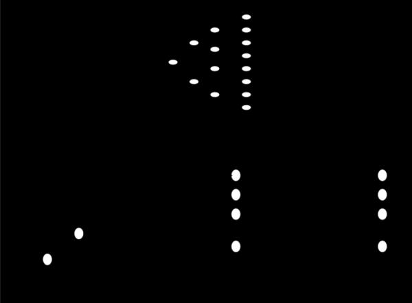
We model actual physical tumor growth, beginning with the clonal expansion of a single cell (Hong et al., 2010; Siegmund et al., 2009), applying a biological constraint on the total number of tumor cells (e.g. assuming 1 billion cells/1 cm³), and making use of clinical data on tumor size to inform our model. Tumors arising from glandular tissues such as the colon, with cells organized into small tubular units, are typically adenocarcinomas which are composed of many neoplastic glands. Adenocarcinomas are also common in the breast, prostate, lung, pancreas, and stomach. As such, dividing cancer cells in our model are geographically confined to cancer glands, which also divide, with constraints on the total number of cells based on the size of the tumor (see figure 1). Our model directly reflects this glandular structure.

Figure 1.

The tumor growth model. Top graph shows the division of the 1^st transformed cell into a gland. The bottom graph shows the exponential growth and the constant-size growth of the glands in one tumor half. See text for more details.

A tumor is simulated as the clonal expansion of a single transformed cell. A 4 cm³ tumor contains approximately 4 billion cells, which is impossible to simulate at the single-cell level by forward simulation. However, the organization of tumor cells within glands allows for a flexible growth modeling across two different scales, cell level and gland level. Since one gland contains approximately 8,000 cells, a 4 cm³ tumor can be approximated by only 500,000 glands. This size is achieved after only 19 generations of exponential growth. We mimic the structure of our sampled data by sampling only eight glands from the ~500,000, and storing their ancestral tree. This is followed by the simulation of single-cells along the ancestral tree for the sampled glands. This approach allows us to simulate for each tumor a sample of ~33K cells (=4,096 cells/gland × 8 sampled glands) instead of a total of ~4 billion. This ensures computational tractability.

The cells and glands follow separate models for growth. We model gland growth as exponential growth followed by a period of constant size (see figure 1) At the cell-level, the single transformed cell undergoes exponential growth (cell doubling) until it attains the number required of the first cancer gland (see figure 1). In subsequent generations, the cells in the gland divide until they double in number, and then the gland divides. Both the cells and glands continue to divide, forming a second period of exponential growth (phase one for gland tree growth), until the tumor reaches its fixed biological size. The tumor then enters the second phase of the gland tree growth, in which the gland number remains constant, but the cells within glands divide and die, allowing for continued ‘aging’ in a tumor of fixed size (no growth). Cell division and death occurs via symmetric and asymmetric division. We refer to long-lived dividing cells lines as cancer stem cell lines. The model for cancer stem cell division is as follows. Under asymmetric division, a cancer stem cell differentiates into one cancer stem cell and one normal cancer cell, while under symmetric division, a cancer stem cell have 0.5 probability to give birth to two cancer stem cells and 0.5 probability to divide into two normal cancer cells. This is parameterized by probability of asymmetric division (PAD) that controls the proportion of cancer stem cells having asymmetric division. Finally, the DNA methylation patterns are sampled from approximately 16 glands per tumor, eight per tumor half. For a detailed mathematical description of the model, see (Siegmund et al., 2009), in which the same parameterization is used.

Our analysis explores variation in a total of five parameters (see Table 1). The remaining model parameters were fixed at either their most likely value or at values reported in the literature. The parameter NCSC is the number of cancer stem cells present in one gland of a tumor. In earlier work we studied how quickly a tumor grows by comparing two different growth models; the first was a two-phase model of exponential growth, followed by constant tumor size, but allowing for cell aging through continued cell division and death, while the second was a slower growing tumor that follows a smooth, Gompertzian (S-shaped) growth curve (Hong et al., 2010). We found little difference in parameter estimates from the more computationally demanding slow-growth model (Hong et al., 2010), and do not pursue it further here. Instead, we explore our ability to estimate parameters that were treated as fixed (at arbitrary values) in our previous work, such as the DNA methylation and demethylation copy error rates. We also focus on our ability to infer the DNA methylation pattern of the ancestral cell.

Table 1.

Parameters in our model

Parameters	Possible Value and Prior Distribution
DNA Methylation Error Rate (MER)	U(0,0.1)
DNA Demethylation Error Rate (DER)	U(0,0.1)
Number of Cancer Stem Cells (NCSC)	2 to the power of 1,2,3,4,5,6,7,8,9
Probability of asymmetric division (PAD, R)	U(0.5,0.1)
Number of generations of constant size (T3)	10 to 365

2.2 Statistical Methods

As the level of detail in models used to answer biological questions grows, due to the increased richness of data and our eagerness to use it to obtain a more comprehensive understanding of the biological phenomena, the computational difficulties of analysis also grows, to the extent that analysis often become intractable. This intractability is frequently caused by the need to calculate the likelihood function – the function that gives the likelihood of the data for a particular combination of model parameters. This has lead to the rising popularity of methods in which, instead of calculation, we use simulation to perform statistical inference. Here, we exploit one of these methods: approximate Bayesian computation [ABC]. The advantage of such methods lies in the fact that simulation generally remains tractable long after the rise in data richness and/or model complexity causes exact calculation to become impossible. The goal of the simulation is to estimate the likelihood directly, for example using so-called Monte-Carlo methods. The very first documented Monte-Carlo simulation was the Buffon's needle experiment to approximate π (Ramaley, 1969), in which the analyst performed a repeated series of experiments in which a needle was tossed onto a table.

Many ABC methods rely upon versions of the Acceptance-rejection Algorithm (Ripley, 1987). Essentially, the goal is to find the joint posterior distribution for the model parameters conditional on the observed data. This characterizes our beliefs about model parameters and states given the observed data. The analysis proceeds by comparing simulated datasets to the data that were observed experimentally and asking what parameter combinations lead to data that matches the observed data. However, for complex data structures exact matches happen very infrequently, even if data is simulated using the correct model and true parameter values. Therefore, ABC methods use an approximation in which ‘near misses’ are also accepted (Beaumont et al., 2002; Marjoram and Tavare, 2006; Tavare et al., 1997).

In this paper we use an ABC form of the Acceptance-rejection Algorithm (d'Onofrio, 2005; Tavare et al., 1997). We aim to find the posterior distribution of parameters θ=(θ₁, θ₂,..., θ_n) based on the data (or sample) D that were observed from experiments. This is written as

$$f(\theta \mid \mathbf{D})=f(\mathrm{D}\mid \theta )\pi \left(\theta \right)∕f\left(\mathbf{D}\right).$$

The likelihood term, ƒ(D|θ), is impossible to obtain in many contexts, including our own, hence our need to exploit ABC. In the ABC scheme, we use summary statistics S=(S₁,S₂,...,S_k) to represent key features of the observed data D, thereby reducing the computational complexity significantly and, in the process, regaining tractability of analysis. The summary statistics used in our analysis are normalized and listed in table 2. So-called ‘Sufficient statistics’ are the best choice for summary statistics if they are available (since then, by definition, ƒ(θ|S)=ƒ(θ|D)). However, in nearly all practical cases sufficient statistics are unavailable. As a consequence, we estimate ƒ(θ|S), for which the analysis is tractable, rather than ƒ(θ|D), for which it is not.

Table 2.

Summary Statistics

S1	Percentage of methylation
S2	Average number of unique tags
S3	Average hamming distance within all glands
S4	Average hamming distance among all glands
S5	Average hamming distances between segments
S6	Average number of transitions
S7	Vector of sitewise percentage of methylation

See definition of each summary statistics in supplemental material.

The ABC version of rejection sampling is as follows:

For i=1 to N

1. Sample parameters θ’ from the prior distribution π(θ)

2. Simulate data D’ using model M with the sampled parameters θ’, and summarize D’ as S’.

3. Accept θ’ if d(S’, S) < ε, for a given threshold ε. Where d(S’, S) is a measure of distance between S’ and S.

4. Go to 1.

After N iterations, a set of accepted parameter values, denoted by θε, is generated, which consists of samples from the posterior distribution ƒ(θ|S’≈S), a statistical approximation to ƒ(θ|S) (Tavare et al., 1997). Ideally, we want to choose as small ε as possible, because the posterior distribution will be as close as possible to ƒ(θ|S). However, the consequence of a small ε is fewer accepted θ’s, leading to a higher level of empirical noise in the estimate of ƒ(θ|S’≈S). In other words, more computation is needed to get a sufficient number of samples from the posterior distribution of interest.

In our paper we use a common variation on the above description. Rather than using a fixed threshold, ε, we sort all N distances calculated in step 3, and accept the θ’ that generated the smallest 100*η percent distances. Such an approach has been used in a variety of ABC papers e.g., (Beaumont et al., 2002; Ripley, 2009).

The question of which statistics to include in an analysis such as this is a subtle one. In principle, given infinite computational resources, adding extra statistics can never hurt, and will always help unless the new statistic is completely correlated with the existing statistics. However, in practice, adding less informative statistics increases the noise in the measure of distance between observed and simulated datasets, and thereby increases the error in the degree of agreement between the empirical estimate of ƒ(θ|S’≈S) and ƒ(θ|S) itself. As such, a small, informative set of summary statistics is best (Fearnhead and Prangle, 2012). The set of summary statistics used in our analysis are given in Table 2. They represent a selection of statistics we have used in similar analyses (Laird, 1964; Siegmund et al., 2011; Siegmund et al., 2009), with some additional statistics designed to be informative regarding questions of particular interest in the present paper. We generate N = 60 million simulations, using the prior distributions shown in Table 1, with the methylation status of the single ancestral cell being randomly generated for each data point, and we accept 0.005% of these simulations (3,000 data sets) to generate the posterior distributions (thereby making ε as small as is reasonably possible) . The distance metric is defined as:

$$\mathrm{d}(\mathbf{S}’,\mathbf{S})={\Vert {(\mathbf{S}’-\mathbf{S})}^{\ast }{\mathbf{W}}^{\mathbf{T}}\Vert }_2,$$

where W is a weight vector. We use equal weights on the seven summary statistics shown in Table 2 for all analysis except that of the ancestral state, where we placed higher weight on S₇, a statistic that is particularly informative regarding ancestor.

3 Results

3.1 Simulated data

To benchmark the performance of our analysis machinery, we begin with an analysis of simulated datasets. By analyzing simulated data we are able to compare summaries of our estimated posterior parameter distributions to the (in reality unobserved) generating parameter values. We describe several such analyses below. For each analysis, in order to help intuition, we begin by presenting some representative, illustrative results for single simulated datasets, before presenting overall results of a more comprehensive simulation study.

3.1.1 Estimation of Ancestor

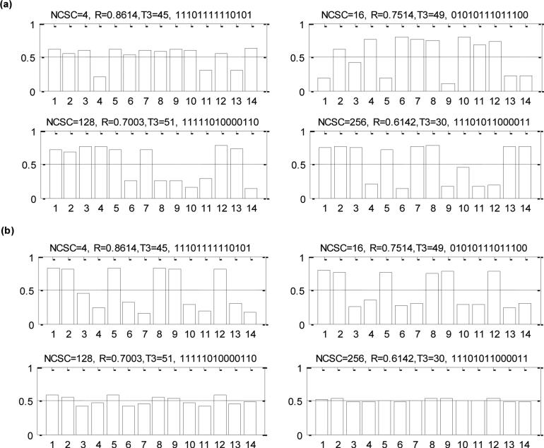
We begin with one of our questions of primary importance: the state of the ancestral cell. This is not, as such, a parameter, but its posterior distribution can be estimated in a way that is directly analogous to the method used for parameters. We assume an uninformative prior distribution for the ancestor - a Bernoulli distribution with p=0.5 at each site. Illustrative results are shown in figure 2a. We show the posterior distribution of the methylation status of each site for four simulated ‘test’ tumors. In our analysis, the number of CpG sites is 14, and the parameters used to generate these four simulated tumors are shown in the title of each figure, using the notation of Table 1 (where the 4^th entry in the title is the ancestral state of the simulated tumor: 1 being methylated; 0 being unmethylated). The height of each bar represents the posterior probability of that site being methylated in the very first transformed tumor cell. The posterior distribution indicates that our analysis retrieves the state of the original cell of the tumor successfully in each case (although, in many cases, not with high confidence). This is more impressive when one considers that there are 2¹⁴=16,384 possible ancestors for each tumor in our simulation.

Figure 2.

(a) Posterior distributions of the estimates for the probability of the initial methylation status being 1 in the ancestors of illustrative simulated tumors (generating parameters are shown above each figure, followed by the DNA methylation pattern of the initial transformed cell). (b) The effect of age on posterior distributions of the estimates for the probability of the initial methylation status being 1 in the ancestors of the simulated tumors.

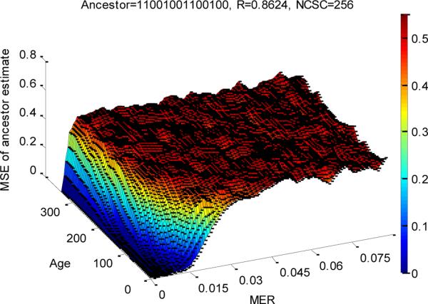
One key feature revealed by our simulations is that the reliability of the estimate of ancestral methylation status depends on the age of the tumor (see figure 2b). When the age of the tumor becomes great, for example T3=240 in figure 2b, the initial methylation status becomes largely not inferable. This is not unexpected. The pattern of observed variation in the final tumor is a complicated perturbation of that in the progenitor cell. Over time, the perturbation becomes greater and greater, until eventually all memory of initial state is lost. (In technical terms, the stochastic process modeling methylation at each site becomes stationary.) The key question, then, is how quickly this memory is lost. In figure 3 we plot the mean square error (MSE) of the most likely ancestral methylation state, compared to the true ancestral state, as a function of tumor age and DNA methylation error rate (MER). As expected, the MSE increases as the tumor becomes older and the MER becomes larger. Note that there is a degree of confounding here. Comparing two tumors, A and B say, if tumor B is twice as old as tumor A, but has a MER that is half that for tumor A, the pattern of variation in the two tumors will be quite similar (since it is related to the expected numbers of changes to methylation status). In figure 3 we see signal regarding the methylation status of the ancestral cell is relatively quickly lost. But if a tumor is young, (Age<100), and MER is low (<0.03), signal regarding ancestral state is present.

Figure 3.

The mean square error of the estimates of the ancestor, NCSC=256, R=0.8624, Ancestor 11001001100100 ( the DER was set to be half of the MER).

3.1.2 Estimation of the methylation and demethylation error rates

Next we explore how quickly methylation and demethylation errors propagate. We simulate a number of tumors with known methylation and demethylation error rates (generated uniformly through 0 to 0.1), with other parameter values kept constant (and assumed as known in the subsequent analysis). We then estimate the posterior distribution for both MER and DER.

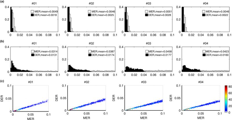
In figure 4 we show example results for four simulated tumors. These were all generated using MER=0.005, DER=0.002, and T3=10, and have posterior distribution for the MER and DER centered at around 0.005 and 0.002 respectively, suggesting that the MER and DER can be correctly estimated in these illustrative cases. Increasing the age of the tumor from T3=10 (figure 4a) to T3=80 (supplemental figure 1a) still results in a good estimate of MER and DER. However, when T3=345 the estimation of MER and DER becomes more difficult (figure 4b). The reason that it appears to become harder to estimate MER and DER for older tumors is that the tumor eventually reaches a stationary phase in which the overall methylation level is largely a function of the relative rates of MER & DER, (expressed through their ratio) rather than the marginal value of either. Thus, a wide range of values for MER is supported provided we choose DER appropriately (i.e., to maintain the necessary ratio – see figure 4c). This flexibility is lost for younger tumors that have not grown for long enough to exhibit this kind of ‘stationarity’ behavior. These conclusions are robust across a range of simulated tumor data, in which ancestral state was also varied (supplemental figure 1b).

Figure 4.

Posterior Distributions of MER and DER. 4 simulated tumors generated under MER=0.005, DER=0.002, NCSC=256, ancestor= 01111101100100, R=0.5 and (a) T3=10; (b) T3=345; (c) top view of the joint distribution of MER and DER from figure 4b.

We note in passing that the shape of the joint distribution of MER and DER provides us with evidence of the age of the tumor. If the joint distribution is clustered into a small cloud, the tumor is still in an early stage in terms of DNA methylation alterations (supplemental figure 3), On the other hand, if the joint distribution forms a line, as in figure 4c, the tumor is older.

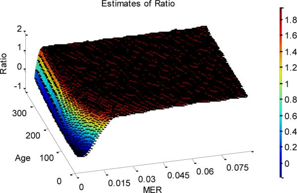
Moving to summary results from the full simulation study, figure 5 summarizes our ability to estimate the ratio MER/DER over a full range of example datasets. We show results for the estimated value of MER/DER over 40 replicates for each combination of parameter values, in which we analyzed data that was simulated with MER/DER=2. We plot the ratio of MER and DER against age and MER. As we can see, we obtain very good estimates of the ratio, except for very low MERs, when, whatever the ratio is (within reason), no changes of methylation state occur (and so accurate inference of relative rates is impossible). As discussed above, because of the fact that patterns of methylation depend largely upon the ratio MER/DER, inference of MER without reference to DER is much less successful.

Figure 5.

The estimate of ratio of MER and DER. The tumors were generated using NCSC=256, R=0.8624, and an ancestor state of 11001001100100, with the ratio of MER and DER set to be 2.

3.1.3 Number of Cancer Stem Cells, probability of Asymmetric division, and Age

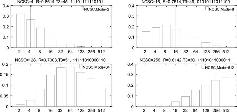
We now consider the remaining model parameters. In figure 6 we focus on estimation of the number of cancer stem cells (NCSC). We show results for 4 illustrative simulated tumors. The results indicate that we can recover NCSC with reasonable accuracy, despite their being a very small fraction of the total cell mass in the tumor. The probability of asymmetric division (PAD), R, plays an important role in establishing the heterogeneity of tumor cells. Our results shed some insight on likely parameter values, but overall results indicate that estimation is difficult (supplemental figure 4a).

Figure 6.

Posterior distributions of the NCSC for four illustrative tumors. The dotted line indicates the true value of NCSC, and the values above each figure indicate the true parameter values.

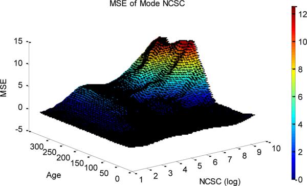
A full simulation study is shown in figure 7. In contrast to results for estimation of ancestral type, the estimation of NCSC is not very sensitive to age when NCSC is small. However, estimation of NCSC (in absolute terms) becomes more difficult when NCSC is high, particularly for old tumors.

Figure 7.

Mean square error of the mode of the posterior distribution of NCSC with respect to varying age and true NCSC. The tumors were generated using MER=0.004, DER=0.002, R=0.8624, and with an ancestral state of 11001001100100

3.2 Experimental data

Having benchmarked the performance of our method using the analysis of simulated data, for which answers are known, we move to an analysis of the experimental data described in section 2.1. We begin by focusing on inference of ancestral state (see figure 8). The estimates show that the ancestral state of the first 5-6 sites of the LOC tag are most likely to be methylated for each patient. The signal regarding state is weakest in CN and CR, suggesting that those tumors are older (see also figure 10). These outcomes support our ability to recover information regarding the ancestral state of tumors, but with the important caveats noted earlier: a) that while this is possible for tumors that have divided, broadly speaking, up to 100 times, this ability is lost for older tumors; b) inference, when possible, is accurate but relatively weak.

Figure 8.

Ancestral inference for experimental data. The x-axis is the CpG site, the y-axis is the probability of each site being methylated in the ancestral cell

Figure 10.

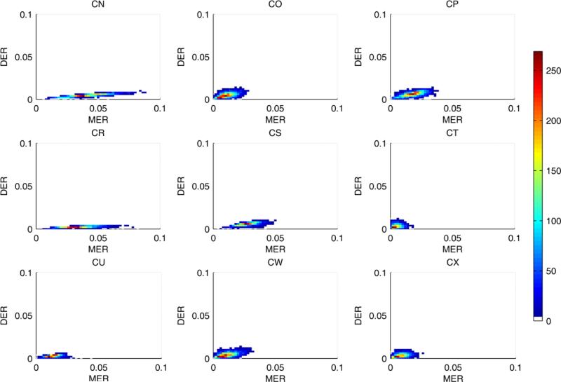
Joint posterior distribution of the DNA methylation and demethylation error rate in the experimental data. It is the top view of the distribution and the color map shows the density.

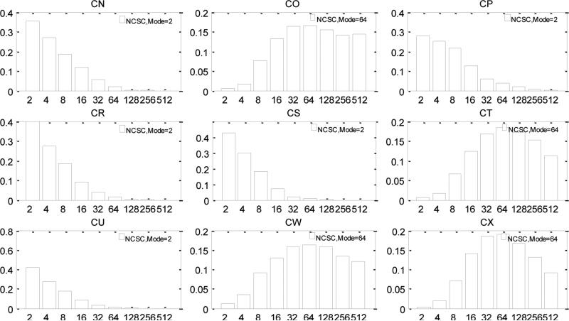
The fact that DNA methylation increases with age suggests that MER is higher than DER (Woo et al., 2009). As shown in figure 9, we do observe that the posterior distribution of MER lies to the right of that for DER. The joint posterior distributions of MER and DER again show the confounding that we observed for the analysis of simulated data ( see figure 10). These results suggest that CN and CR are older than the other tumors (c.f. the discussion of figure 4c). Both MER and DER vary between tumors, suggesting either a patient-specific profile of tumor progression or that the tumors are of significantly different ages. The variability of MER is much larger than DER, but this may simply reflect that, as noted earlier, posterior variance increases with magnitude of MER (DER). The estimated NCSC values also show a patient specific pattern (see figure 11). Tumors CN, CR, CS and CU have very small numbers of cancer stem cells. The remaining tumors appear to have many more cancer stem cells in each gland. The posterior distributions of PAD and T3 for these tumors are shown in supplemental figure 5.

Figure 9.

Marginal posterior distribution of the DNA methylation and demethylation error rate in the experimental data.

Figure 11.

The posterior distributions of the number of cancer stem cells in experimental data. The x-axis is the number of cancer stem cells.

4 Discussion

Tumorigenesis is a complex process that requires considerable effort to decipher. This is particularly true since we typically observe data from a single time-point at the end of tumor growth, rather than being able to watch the tumor as it grows (at least in human subjects). Here, we presented a model, and analysis method, that can be used to study the ancestral state, the methylation error rate, and the number of the cancer stem cells in individual tumors. The former is of particular importance because it is possible it might contain important prognostic flags for future tumor behavior

In previous papers, researchers derived point estimates of a given parameter by fixing other parameters based on prior knowledge (Siegmund et al., 2009). The results inevitably depend on the quality of the prior knowledge that is used. In this paper, we presented an ABC scheme that allows us to obtain inference on the model parameters simultaneously when desired. Of course, some parameters are harder to estimate than others, because they leave less of signal in the observed experimental data. Furthermore, the ability to estimate a feature of tumor growth may depend upon the age of the tumor. For example, we found that the ability to infer likely methylation status of the ancestral cell decreases as the tumor ages (and, in essence, forgets where it started from).

Parameter confounding is also an issue. If we have two tumors, A and B, with A being twice as old as B, but with MER/DER rates that are half as high as those for B, then the properties of the final patterns of variation will be very similar. (This is related to the concept of non-identifiability in statistics.) Consequently, we propose that the measure of age most relevant here is to think of the expected number of changes to methylation status, say. This is the product of the methylation/demethylation rate and the number of cell divisions.

Our analysis shows that we can obtain informative posterior distributions for methylation error rate and the ancestral state for experimentally observed tumor data, provided the tumors are not so old that information regarding ancestor is lost. Therefore, we have shown that, even though we cannot observe the early stages of tumor growth directly, important features of that growth may be inferred by careful analysis of data collected from the tumor at a later time.

The cancer stem cell, being a long-lived dividing cell, is the primary engine driving the tumor to develop. Therefore, understanding how many cancer stem cells there are in a tumor will reveal tremendous amount of information on tumor progression. Experimentally, researchers perform xenotransplantation using markers CD133⁺ to count the NCSC. In our study, the NCSC is retrieved through careful analysis of data under a model for the tumor's natural history. Our analysis show less than 2.5% of cells are likely to be cancer stem cells (the mode of the posterior distribution divided by the number of cells in one gland). This confirms experimental results (Ricci-Vitiani et al., 2006). However, within this constraint, the NCSC appears to vary across tumors (see figure 11). In particular, our experimental data appears to fall into two classes: one for which the NCSC appears to be most likely to take a very low value (2); another in which higher values are best supported (32-128). This suggests different organization patterns and progressiveness may exist in different tumors. Siegmund, Marjoram et al. 2011 showed that MMR deficient tumors (CR and CU) have low NCSC (Siegmund et al., 2011). This is confirmed by our analysis that CR and CU's posterior distributions are concentrated on small NCSC.

One interesting statistical question arises during an analysis such as this: which summary statistics should be used for the analysis? In this paper we have presented results for particular choices of statistics that were most informative for the particular problem at hand. However, if statistics are chosen poorly, quality of inference will suffer. We discuss this at greater length in Supplemental Material for the case of inference of ancestral state. Development of rigorous procedures for choice of statistics, as a function of analysis question at hand, is an area of active research (Barnes et al., 2012; Fearnhead and Prangle, 2012; Hong et al., 2010; Joyce and Marjoram, 2008; Jung and Marjoram, 2011).

In summary, the parameters of tumor growth, and the early stages of tumor growth play an important role in the patterns of variation seen in tumors. They may also carry important prognostic information. This has been hard to assess since the early stages of tumor growth are not typically observed. Our results show that with careful statistical analysis we can obtain estimates of both tumor growth parameters, (captured in terms of full posterior distribution rather than simple point estimates), and of the initial methylation status at loci (which is impossible to observe directly). Our hope is that the ability to do this may open new avenues by which understanding of tumor growth, and future behavior, might be better understood.

Author Highlights.

• The ability to retrieve ancestral information depends on the parameter being inferred and the “age” of the tumor.

• We more successfully retrieve the ancestor state and methylation error rate from younger tumors.

• The methylation and demethylation error rate ratio can be more easily estimated in older tumors that reach stationary phase.

• The number of cancer stem cells can be inferred in most tumors and our analysis suggests it varies significantly between human tumors.

References

- Ambrosi D, Preziosi L. On the closure of mass balance models for tumor growth. Mathematical Models and Methods in Applied Sciences. 2002;12:737–754. [Google Scholar]
- Anderson A, Chaplain M, Rejniak K, Fozard J. Single-cell-based models in biology and medicine. Mathematical Medicine and Biology. 2008 [Google Scholar]
- Barnes CP, Filippi S, Stumpf MP, Thorne T. Considerate approaches to constructing summary statistics for ABC model selection. Statistics and Computing. 2012;22:1181–1197. [Google Scholar]
- Beaumont MA, Zhang W, Balding DJ. Approximate Bayesian computation in population genetics. Genetics. 2002;162:2025–35. doi: 10.1093/genetics/162.4.2025. [DOI] [PMC free article] [PubMed] [Google Scholar]
- Bromham L, Penny D. The modern molecular clock. Nature Reviews Genetics. 2003;4:216–224. doi: 10.1038/nrg1020. [DOI] [PubMed] [Google Scholar]
- Byrne H, Preziosi L. Modelling solid tumour growth using the theory of mixtures. Mathematical Medicine and Biology. 2003;20:341–366. doi: 10.1093/imammb/20.4.341. [DOI] [PubMed] [Google Scholar]
- d'Onofrio A. A general framework for modeling tumor-immune system competition and immunotherapy: Mathematical analysis and biomedical inferences. Physica D: Nonlinear Phenomena. 2005;208:220–235. [Google Scholar]
- Fearnhead P, Prangle D. Constructing summary statistics for approximate Bayesian computation: semi-automatic approximate Bayesian computation. Journal of the Royal Statistical Society: Series B (Statistical Methodology) 2012;74:419–474. [Google Scholar]
- Hong YJ, Marjoram P, Shibata D, Siegmund KD. Using DNA methylation patterns to infer tumor ancestry. PloS one. 2010;5:e12002. doi: 10.1371/journal.pone.0012002. [DOI] [PMC free article] [PubMed] [Google Scholar]
- Joyce P, Marjoram P. Approximately sufficient statistics and Bayesian computation. Statistical Applications in Genetics and Molecular Biology. 2008;7 doi: 10.2202/1544-6115.1389. [DOI] [PubMed] [Google Scholar]
- Jung H, Marjoram P. Choice of summary statistic weights in approximate Bayesian computation. Stat Appl Genet Mol Biol. 2011;10 doi: 10.2202/1544-6115.1586. doi:10.2202/1544-6115.1586. [DOI] [PMC free article] [PubMed] [Google Scholar]
- Klein CA, Hölzel D. Systemic cancer progression and tumor dormancy: mathematical models meet single cell genomics. Cell Cycle. 2006;5:1788–1798. doi: 10.4161/cc.5.16.3097. [DOI] [PubMed] [Google Scholar]
- Laird AK. Dynamics of tumour growth. British journal of cancer. 1964;18:490. [Google Scholar]
- Marjoram P, Donnelly P. Human demography and the time since mitochondrial Eve. Institute for Mathematics and Its Applications. 1997;87:107. [Google Scholar]
- Marjoram P, Tavare S. Modern computational approaches for analysing molecular genetic variation data. Nat Rev Genet. 2006;7:759–70. doi: 10.1038/nrg1961. doi:10.1038/nrg1961. [DOI] [PubMed] [Google Scholar]
- Navin N, Kendall J, Troge J, Andrews P, Rodgers L, McIndoo J, Cook K, Stepansky A, Levy D, Esposito D. Tumour evolution inferred by single-cell sequencing. Nature. 2011;472:90–94. doi: 10.1038/nature09807. [DOI] [PMC free article] [PubMed] [Google Scholar]
- Pritchard JK, Seielstad MT, Perez-Lezaun A, Feldman MW. Population growth of human Y chromosomes: a study of Y chromosome microsatellites. Molecular Biology and Evolution. 1999;16:1791–1798. doi: 10.1093/oxfordjournals.molbev.a026091. [DOI] [PubMed] [Google Scholar]
- Ramaley J. Buffon's noodle problem. The American Mathematical Monthly. 1969;76:916–918. [Google Scholar]
- Ricci-Vitiani L, Lombardi DG, Pilozzi E, Biffoni M, Todaro M, Peschle C, De Maria R. Identification and expansion of human colon-cancer-initiating cells. Nature. 2006;445:111–115. doi: 10.1038/nature05384. [DOI] [PubMed] [Google Scholar]
- Ripley B. Stochastic Simulation. 1987. Wiley; New York: 1987. [Google Scholar]
- Ripley BD. Stochastic simulation. 2009 Wiley.com.
- Shibata D. Inferring human stem cell behaviour from epigenetic drift. The Journal of pathology. 2009;217:199–205. doi: 10.1002/path.2461. [DOI] [PMC free article] [PubMed] [Google Scholar]
- Shibata D, Tavaré S. Counting divisions in a human somatic cell tree: how, what and why. Cell Cycle. 2006;5:610–614. doi: 10.4161/cc.5.6.2570. [DOI] [PubMed] [Google Scholar]
- Shibata DK, Lieber MR. Is there any genetic instability in human cancer? DNA repair. 2010;9:858. doi: 10.1016/j.dnarep.2010.04.011. [DOI] [PMC free article] [PubMed] [Google Scholar]
- Siegmund KD, Marjoram P, Tavare S, Shibata D. High DNA methylation pattern intratumoral diversity implies weak selection in many human colorectal cancers. PLoS One. 2011;6:e21657. doi: 10.1371/journal.pone.0021657. doi:10.1371/journal.pone.0021657. [DOI] [PMC free article] [PubMed] [Google Scholar]
- Siegmund KD, Marjoram P, Woo YJ, Tavare S, Shibata D. Inferring clonal expansion and cancer stem cell dynamics from DNA methylation patterns in colorectal cancers. Proc Natl Acad Sci U S A. 2009;106:4828–33. doi: 10.1073/pnas.0810276106. doi:10.1073/pnas.0810276106. [DOI] [PMC free article] [PubMed] [Google Scholar]
- Tavare S, Balding DJ, Griffiths RC, Donnelly P. Inferring coalescence times from DNA sequence data. Genetics. 1997;145:505–18. doi: 10.1093/genetics/145.2.505. [DOI] [PMC free article] [PubMed] [Google Scholar]
- Woo YJ, Siegmund KD, Tavaré S, Shibata D. Older individuals appear to acquire mitotically older colorectal cancers. The Journal of pathology. 2009;217:483–488. doi: 10.1002/path.2506. [DOI] [PMC free article] [PubMed] [Google Scholar]
- Yatabe Y, Tavaré S, Shibata D. Investigating stem cells in human colon by using methylation patterns. Proceedings of the National Academy of Sciences. 2001;98:10839–10844. doi: 10.1073/pnas.191225998. [DOI] [PMC free article] [PubMed] [Google Scholar]
Associated Data
This section collects any data citations, data availability statements, or supplementary materials included in this article.