Stimulus features, resetting curves, and the dependence on adaptation

Abstract

We derive a formula that relates the spike-triggered covariance (STC) to the phase resetting curve (PRC) of a neural oscillator. We use this to show how changes in the shape of the PRC alter the sensitivity of the neuron to different stimulus features, which are the eigenvectors of the STC. We compute the PRC and STC for some biophysical models. We compare the STCs and their spectral properties for a two-parameter family of PRCs. Surprisingly, the skew of the PRC has a larger effect on the spectrum and shape of the STC than does the bimodality of the PRC (which plays a large role in synchronization properties). Finally, we relate the STC directly to the spike-triggered average and apply this theory to an olfactory bulb mitral cell recording.

1 Introduction

White noise or Wiener kernel analysis is a commonly used method to study the response properties of neurons and to discover the stimulus features to which a neuron best responds ([1–6]). In this analysis, the neuron is subjected to a broadband signal (e.g., white noise) and the statistics of the stimulus conditioned on the firing of the neuron are calculated. For example, the first moment of the stimulus conditioned on the spike is called the spike-triggered average (STA). The STA is easily determined and, for the case of a weak stimulus, provides a model for how a neuron responds to arbitrary stimuli [7]. This type of analysis implicitly assumes that the neuron responds to a single feature and that the response probability density is just the projection of the stimulus onto the STA. The spike-triggered covariance (STC) provides more information about the stimulus features as it incorporates the second order statistics of the spike-conditioned stimulus. Here, the features are extracted via principle component analysis as the eigenvectors of the covariance matrix. These eigenvectors provide a richer and more detailed view of the coding properties of the neuron [4,5,8,9].

These first and second order stimulus-response correlations are generally sufficient to draw conclusions about the so-called feature space of the neuron. However, neurons can also be viewed as dynamical systems [10] with firing properties determined by the combinations of ionic channels that comprise the membrane. Relating dynamics to coding and feature detection is an active area of recent research. [5] were among the first to compute the STA and the STC in a biophysical model, in their case, the Hodgkin-Huxley (HH) model. They numerically extracted the STA and the eigenfunctions of the STC by driving the model neuron with white noise. [11] found the STA for the leaky integrate-and-fire (LIF) model neuron under arbitrary amplitude white noise stimuli. More recently, [12] have attempted to relate the biophysics of neurons to these statistical coding properties. They start by linearizing an arbitrary conductance-based model around a fixed point and then relate the dynamics of the linearized system to the eigenfunctions of the covariance matrix. They extend this analysis to the case where there is a single nonlinearity, the threshold crossing. In a recent paper, [13] studied the noisy LIF model. Specifically, they used the static firing rate-current (FI) curve and the linear response function for the LIF model to make a so-called linear-nonlinear (LN) model; whereby the output rate of the neuron is given by:

$$r(t)=F({\int }_0^{\infty }D(\tau )s(t-\tau )d\tau )$$

where s(t) is the input. The functions F and D(τ) were given by the static FI curve and the linear response, which have been analytically determined for the LIF model [13]. The usual method of deriving an LN model is through reverse correlation (RC) analysis. [13] demonstrated that the RC-determined LN models matched the analytically-determined LN models very well. [9] used a complicated analysis of the Fokker-Planck equation (assuming large noise, they perform stochastic linearization) to compute the STA for a variety of models, including the LIF and the quadratic integrate-and-fire (QIF) models, thus relating the spiking dynamics of the neuron to its coding of features. In an approach related to the present paper, [8] used phase resetting curves (PRCs) for the normal forms of type I and type II neurons to compute the covariance matrix and extract the features from the resulting matrix. They compare the eigenvalues and eigenfunctions by driving the phase models with strong noise.

One of the most common behaviors of neurons and models of neurons is repetitive firing, where the neuron fires spikes in a periodic manner. Dynamically, this type of firing corresponds to an exponentially stable limit cycle. Weak stimuli applied to a periodically firing neuron shift the timing of the spikes in a way that is characterized by the PRC. If the inter-spike interval (ISI, or period) of the neuron is T, then the PRC, denoted by Δ(t), is a T–periodic function which tells you the amount of time the next spike will be shifted given that a perturbation occurs at a time t since the last spike. Thus, the PRC characterizes the way that stimuli shift the timing of spikes in the same manner that the STA characterizes the way that stimuli modulate the firing rate of a neuron. Since changes in the timing between spikes is equivalent to changes in the instantaneous firing rate (the reciprocal of the ISI), it seems natural that there is a relationship between the STA and the PRC. In [14], we found this relationship by using a perturbation expansion assuming that the noise was weak. Specifically, we found that:

$$\text{STA}(t)=-{\sigma }^2{\int }_0^T{\mathit{\Delta }}^{\prime }(s)C(T-t-s)ds$$

where C(t) is the autocorrelation of the noise. In particular, if the noise is white

$$\text{STA}(t)=-{\sigma }^2{\mathit{\Delta }}^{\prime }(T-t).$$

In this paper, we extend the theory developed in [14] to determine the STC of a weakly perturbed neural oscillator. We first illustrate the calculations on the HH model. We then use the approximation to explore the systematic changes in the features as we vary the type and shape of the PRC of a spiking model. We use a theta model with adaptation [18] which has the effect of both skewing the PRC to the right and creating a prominent negative lobe right after spiking. Since there is no analytical form for the PRCs in either the HH or theta models, we then look at a simple parameterized family of PRCs:

$$\mathit{\Delta }(t)=exp(b(t-2\pi ))(sin(a)-sin(t+a)).$$

We choose this family as it covers the generic forms of so-called type I and type II neural oscillators (see [15,8,16]) and has recently been used to fit the PRCs of olfactory bulb mitral cells [17]. In both models, we find qualitative changes in the first several eigenvectors of the STC as the PRC changes shape. Thus, small changes in the shape of the PRC lead to changes in the feature selectivity of the neuron. Finally, we use the relationship between the STA and the PRC along with that of the STC and the PRC to directly relate the STC to the STA. We apply this method to the HH model and to a recording of an olfactory bulb mitral cell.

2 Methods

We simulate model neurons by driving them with filtered white-noise stimuli of the form:

$$\frac{d\xi }{dt}=-\xi /\tau +\frac{1}{\sqrt{\tau }}\frac{dW(t)}{dt}$$

where W(t) is white noise and τ is generally between 0.05 and 0.5 ms. (We use filtered noise as it results in smoother plots and faster convergence. Using different values of τ, as long as it is sufficiently small, produced quantitatively similar results.)

Consider a general weakly forced neural oscillator,

$$\frac{dX}{dt}=F(X)+\epsilon \xi (t)Y$$ (1)

where X represents the neural model, ξ(t) is the noisy input, ε is a small positive parameter, and Y is the vector that is zero except in the component corresponding to the voltage where it is 1. (For example, if X represents the components of the HH equations, Y is (V, m, n, h) and only the V –component receives inputs.) When ε = 0, assume that there is a stable limit cycle, X₀(t) with period T. For small ε, we can write, X(t) = X₀(θ) + O(ε) and obtain the following equation for the phase, θ [19]:

$$\frac{d\theta }{dt}=1+\epsilon \xi (t)\mathit{\Delta }(\theta )$$ (2)

where Δ(θ) is the infinitesimal PRC.

In our simulations, we will generally use (2), but for comparison, we will also use the full biophysical model, (1). The function Δ(θ) is numerically found from equation (1) by solving the associated adjoint equation [20] using XPP [21]. Since Δ(θ) is numerically determined and in our theory we need derivatives of Δ(θ), we write it as a truncated Fourier series (between 40 and 100 terms) and then differentiate them term by term.

To compute the STA and the STC, we collect up to a million spikes of (1) or crossings of 0 modulo T for (2) and use the signal, ξ(t), for the T ms preceding each spike to get the STA:

$$\text{STA}(t)={\langle \xi (t_{sp}-t)\rangle }_{t_{sp}}$$

where the average is over all spikes whose times are the t_sp’s. Similarly, we compute:

$$\text{STC}({\tau }_1,{\tau }_2)={\langle \xi (t_{sp}-{\tau }_1)\xi (t_{sp}-{\tau }_1)\rangle }_{t_{sp}}-\text{STA}({\tau }_1)\text{STA}({\tau }_2).$$

We use MATLAB to compute the eigenvalues and eigenvectors for the resulting matrix.

We used two different spiking models to explore further the theory. We started with a standard HH model and applied a current of I = 10 μA/cm² to generate periodic firing with a period of about 14 ms. We integrated the HH model with a time-step of 0.05, so that over one period, we had 294 points. The STC matrices were 294 ×294. In addition to the HH model, we used a variant of the theta model that has a negative feedback to mimic spike frequency adaptation [18]:

$$\begin{array}{l}\frac{d\theta }{dt}=1-cos\theta +(1+cos\theta )(I-gz)\\ \frac{dz}{dt}=(exp(-4(1+cos(\theta +2)))-z)/5.\end{array}$$

For this model, we covaried I and g so that the period remained fixed at 7.06. (The period has no dimensions as this is a dimensionless model.) For the theta model, we integrated the equations with a time step of 0.01, so that the PRCs were discretized into 707 points. The STC matrix was approximated as a 707 × 707 matrix.

Finally, to explore explicit PRCs, we first used the family [17]:

$$\mathit{\Delta }(\theta )=(sina-sin(\theta +a))exp(b(x-2\pi )).$$

With positive values of the parameter b, the PRC is skewed to the right so that it is close to zero in the first half of the cycle. We either fixed b = 0.5 and varied a or fixed a = π/2 and varied b. When b = 0, we recover the family of PRCs that has been used in many papers studying the synchronization of oscillators and their responses to noise [15,22,16,8]. We approximated the STC matrix for these models as 100 × 100 and to check accuracy, 200 × 200.

3 Results

3.1 Theory

In our previous work [14], we computed the STA from the PRC and obtained

$$\text{STA}(t)=-{\epsilon }^2{\mathit{\Delta }}^{\prime }(T-t).$$ (3)

For completeness, we include this calculation in the appendix. The other main theoretical result is that we can also compute the STC using a similar expansion. We present this in the appendix. This calculation results in the following equation for the STC:

$$\text{STC}(t_1,t_2)={\epsilon }^{2}C(t_2-t_1)+{\epsilon }^4{\mathit{\Delta }}^{″}(T-t_2)\mathit{\Delta }(T-t_1)H_0(t_2-t_1)+{\epsilon }^4{\mathit{\Delta }}^{″}(T-t_1)\mathit{\Delta }(T-t_2)H_0(t_1-t_2).$$ (4)

Here H₀(t) is the Heaviside step function with the proviso that H₀(0) = 1/2. We can drop the T as Δ and its derivatives are T–periodic. C(t) is the autocorrelation of the stimulus. A similar formula appears in [23], but no details of the derivation are provided. We therefore include these calculations and their associated assumptions in the Appendix for completeness.

3.2 HH equations

The HH equations are an example of a so-called Class II excitable system [10]. That is, the onset to repetitive firing is through a subcritical Andronov-Hopf bifurcation (HB). The PRC for the normal form of the HB was computed by [24] and is proportional to sin(θ). Several recent papers [5,8] have computed the STA and the STC for the HH equations. In the former study, they drove the excitable HH system (zero applied current) with sufficient noise to get spiking while in the latter study, the model was in the oscillatory regime.

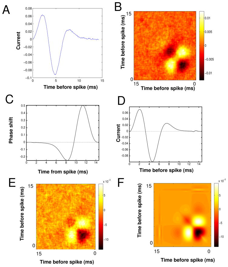
Figure 1 shows results of our own analysis and simulations of the HH model. We inject the model equations with a constant current so that there is regular spiking and then with the filtered white noise stimulus. The coefficient of variation of the ISI was 0.15. Figure 1A shows the STA computed from 1.2 × 10⁶ spikes with a noise amplitude of 1 μA/cm² and τ = 0.5 ms. Panel B shows the STC with the autocorrelation of the stimulus removed. Before continuing we note that even though our simulations have rather small noise and are in the oscillatory regime, the STC of panel B is qualitatively similar to the STC in Figure 8 of [5] with many of the same details. Figure 1C shows the numerically computed infinitesimal PRC (periodic solution to the adjoint operator) for the HH model. As many have noted, the HH model is so-called type II, with a large region where the phase is retarded followed by a phase advance. Using equation (3), we can approximate the STA for the HH model and this is shown in Figure 1D. The shape and magnitude are almost identical up to some fine features near the tail. This confirms the utility of the calculations from [14]. We also remark that the STA computed in [5], Figure 7, looks like an attenuated version of Figures 1A,D. Figure 1E shows the STC as computed from the phase model (2) using the Δ(θ) obtained from the HH equations, namely, the curve shown in Figure 1C. Despite its being a simple one-dimensional representation of the full four-dimensional spiking model, the phase model does a very good job of capturing the STC of the full spiking model. (The STC requires higher order terms which are not included in the phase reduction, so it is a bit surprising that Figures 1B and E are so similar. See the caveats discussed in the Appendix.) Figure 1F shows the STC computed using equation (4). Almost all the quantitative and qualitative features of the simulated STC are captured by the asymptotic formula and given the similarity between panels E and B, the equation (4) appears to be a close approximation to the STC for the full spiking model.

Fig. 1.

HH example. (A) STA for the HH equation (Noise level, σ² = 1 mV²/ms, τ = 0.2 ms, I = 10 μA/cm²); (B) STC with the stimulus correlation subtracted from the diagonal; (C) PRC for the HH model; (D) STA from equation (3); (E) STC for the phase model (2) using the PRC for the HH model; (F) STC from equation (4).

Fig. 7.

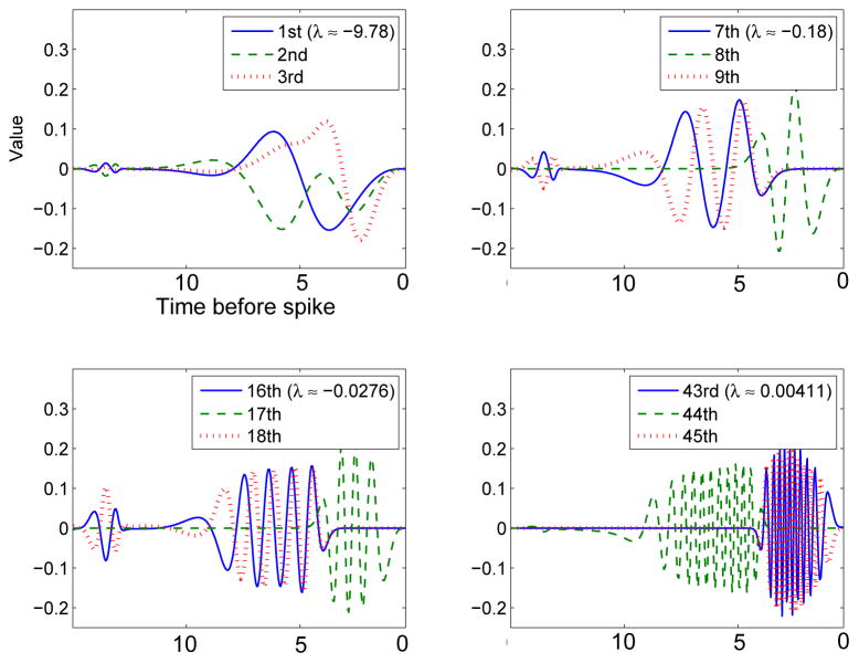
Higher order eigenvectors of the theta model with no adaptation (compare figure 6 with g = 0).

These simulations and calculations show that even for reasonably strong noise (σ² = 1 mV²/ms), the asymptotic formulae (3) and (4), which depend on a phase reduction, work quite well for the full HH model. Given this confirmation, we turn to a discussion of the spectra of the covariance matrix, how it depends on parameters, and what it tells us about the features to which the neuron is sensitive.

3.3 Eigenvectors

The eigenvectors of the covariance matrix provide a set of features to which the neuron is sensitive [5] as well as providing a set of filters for linear-nonlinear models [5,13]. In real neurons and simulated biophysical models, the STC is a finite-dimensional matrix as it is necessary to discretize time in both cases. Equation (4) provides a continuous representation of the STC so that the eigenvectors are actually eigenfunctions and solutions to a linear integral equation:

$$\begin{array}{l}\lambda u(t)={\int }_0^{T}C(t,s)u(s)ds\\ ={\epsilon }^4\left[\mathit{\Delta }(-t){\int }_0^t{\mathit{\Delta }}^{″}(-s)u(s)ds+{\mathit{\Delta }}^{″}(-t){\int }_t^T\mathit{\Delta }(s)u(s)ds\right].\end{array}$$ (5)

The general eigenspectrum of (5) is not possible to determine except in some special cases. Suppose that the PRC has the form Δ(θ) = sin(θ + c) where c is a phase-shift. (Note that only c = 0, π satisfy the requirement that Δ(0) = 0.) If this is the case, then Δ″(θ) = −Δ(θ) so that equation (5) becomes the simple separable model:

$$\lambda u(t)=-{\epsilon }^{4}sin(t+c){\int }_0^{2\pi }sin(s+c)u(s)ds$$ (6)

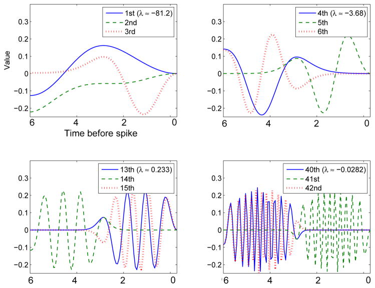
and the only nonzero eigenvector is u(t) = sin(t + c) and λ = −ε²π. All other eigenvectors are zero. Thus, the pure sinusoidal case is degenerate. PRCs that contain other Fourier components will have a complete set of eigenvectors. Figure 2 illustrates some of the eigenvectors for the STC of the HH equations using equation (4) to create the covariance matrix. As we go to higher order eigenvalues, we see two effects: the eigenvectors get more and more oscillations and they shift from times right before the spike for odd modes to times about a half a period preceding the spike for even modes. The localization and the frequency of oscillations suggest that projections onto these eigenvectors are reminiscent of a wavelet transform. We finally note that the first eigenvector (upper left panel, solid line) is very similar in shape to that found in [5] figure 12; this is somewhat surprising as our stimuli are weakly applied to an oscillatory neuron and their results are for strong stimuli applied in the excitable regime. We also note that, like we find, their higher order eigenvectors have more oscillations.

Fig. 2.

Some of the eigenvectors of the STC for the HH model computed using the numerically computed adjoint. The eigenvalues are ordered according to their magnitude.

3.4 Dependence on the adaptation current

We now use equation (4) to explore how a small amount of slow adaptation current alters the first few eigenvectors of the covariance matrix. We use the theta model with adaptation, a simple spiking model equivalent to the Izhikevich model with an infinite spike threshold and reset. We first illustrate how adaptation affects the shape of the infinitesimal PRC or the adjoint of the model neuron. We vary the slow adaptation current while at the same time varying the applied current so that the period of the oscillation remains the same, in this case, about 7.06. Figure 3 shows that for small values of the current (g < 0.5), the main effect is to skew the PRC to the right. Note that with zero adaptation, the PRC is nearly symmetric about the midline. As the adaptation gets large, the PRC increases dramatically in magnitude and attains a large negative lobe (g = 2, 3). We will see shortly that it is, in fact, the skew that matters most with respect to the STC and its eigenvalues.

Fig. 3.

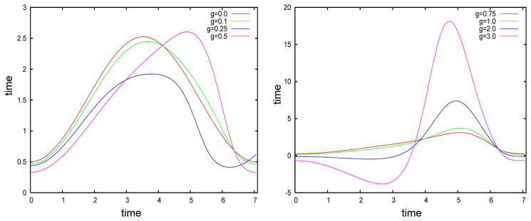
The infinitesimal PRC or adjoint for the theta model with different levels of adaptation. Adaptation strength is noted in the key.

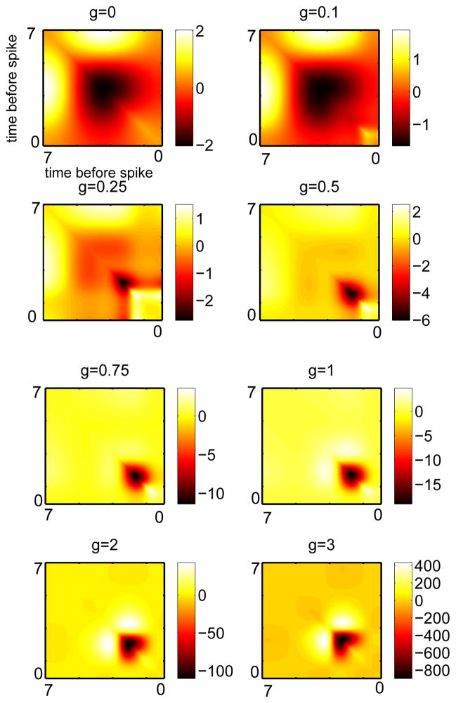
Using (4), we compute the STC for each of these PRCs, the eigenvalues of the resulting matrices, and the first few eigenvectors for each matrix. Figure 4 shows the approximated covariance matrices for this model as the adaptation increases. At very low or zero values of adaptation, there is a large negative region in the center of the STC with two symmetric positive lobes. As the adaptation increases, the negative lobe gradually shrinks and moves toward more distant times with respect to the spike. Once the adaptation gets past about g = 0.5 (the point at which adaptation begins to mainly affect PRC magnitude rather than PRC skewness), the STC changes little except in its magnitude. The two positive side lobes of the STC move inward toward the diagonal and the negative part is dominant at the distant times.

Fig. 4.

Approximated covariance matrix for the theta model with different levels of adaptation. The largest qualitative differences occur with the addition of small levels of adaptation.

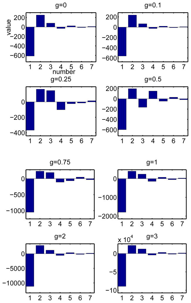
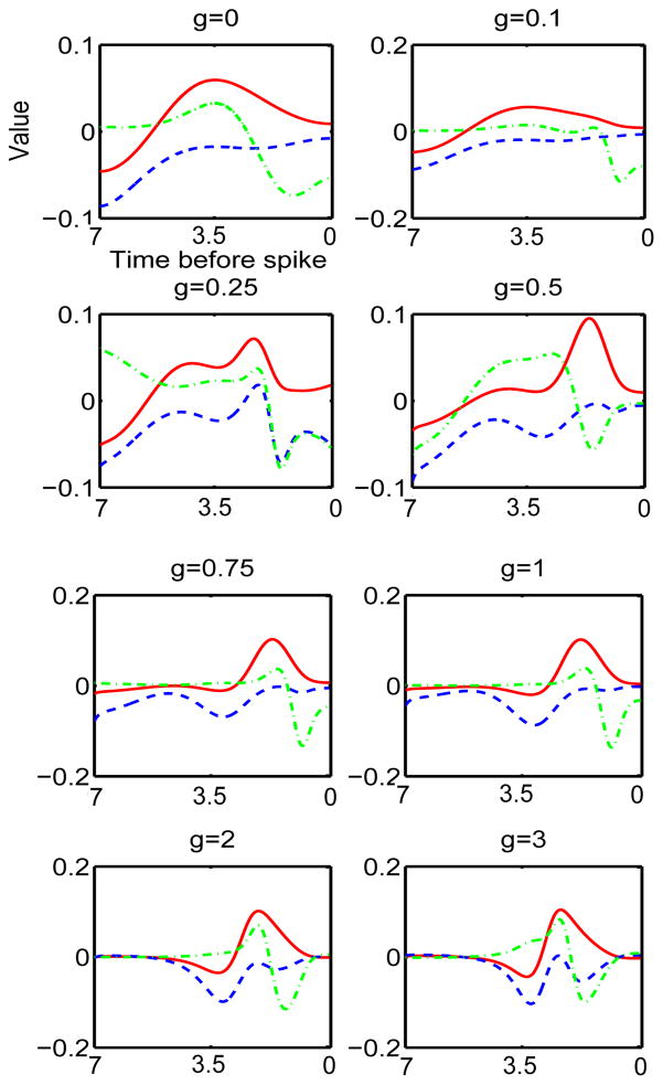
Figure 5 illustrates the first seven eigenvalues of the STC sorted according to their magnitude. The first eigenvalue is always negative and the second is positive. The others seem to change sign, although, other than scaling, they settle into roughly the same pattern and ratio once g exceeds about 0.5. The first three eigenvectors are shown in Figure 6. As adaptation increases, the first eigenvector (blue dashed) becomes compressed with a peak toward the distant time and then becomes bimodal. In many ways, it resembles the PRC itself (compare with Figure 3), a result observed in [8]. The second eigenvector (green, dash-dot) gets more lobes in it but remains bimodal. The third eigenvector (red) seems to be like the first eigenvector but shifted to the later times.

Fig. 5.

First seven eigenvalues of the approximate covariance matrix for the theta model with different levels of adaptation. The largest qualitative differences occur with the addition of small levels of adaptation.

Fig. 6.

First three eigenvectors for the covariance matrix for the theta model with different levels of adaptation. First eigenvector is blue, second is green, third is red.

As a qualitative comparison between general features of the eigenspectrum, we look at some of the higher modes of the covariance matrix for the pure type I model (g = 0). Figure 7 shows some of the higher order eigenvectors for the theta model. Like those of the HH model, higher modes alternate from close to the onset of the spike to a half-cycle away and have more and more oscillations.

In sum, we see that adaptation-dependent changes in the shape of the STC occur primarily at low values of adaptation. The dominant eigenvectors change, but seem to converge to qualitatively similar shapes once g exceeds 0.75. It is interesting to note that the PRC first becomes bimodal (a negative and positive lobe) only when g is around 2. But by the time g = 2, there are few changes in the STC and its spectrum. This is somewhat surprising, as PRCs with a large negative lobe have quite different synchronization properties than do those that are strictly positive ([15,16,25]). Thus, there is not an obvious relationship between the synchronization properties (which depend on PRC type) of neurons and the stimulus features that they are sensitive to. Clearly, there is a relationship between the shape of the STC and its spectral properties and the PRC, but it is not a simple one.

3.5 Simple parametrizations

We now explore the spectral properties of the STC for a class of parameterized PRCs:

$$\mathit{\Delta }(\theta )=exp(b(\theta -2\pi ))(sin(a)-sin(a+\theta )).$$ (7)

When b = 0, we have the standard parameterization going from type II (a = 0; negative and positive values) to type I (a = π/2; nonnegative) [26]. The parameter b > 0 skews the PRCs to the right. This parameterization (along with a scaling factor) was used to great utility to fit the PRCs recorded from olfactory bulb mitral cells in [17]. While it fits nicely, it has the problem that if b ≠ 0, it is not a periodic function.

We first look at b = 0. When a = b = 0, the STC is degenerate since it is then a product of sines (c.f. equation (6)). Thus, we set b = .0001 to remove the degeneracy.

Figure 8 shows how the first four eigenvalues change with a for (7). The dominant (first) eigenvalue (black) is strictly negative while the second one (blue) is positive. The third and fourth are also of one sign and are small in magnitude compared to the first one. (The apparent switch in colors is an artifact of our sorting algorithm which uses magnitude of the eigenvalues and does not enforce continuity. Thus, there is no actual discontinuous switch.) We remark that in this parameterization, since b = 0, there is no change in skew of the PRC. The right panels of Figure 8 show the first and second eigenvector. The color indicates the magnitude of the eigenvector. The parameter a runs down. One can see that for the first eigenvector, the dominant positive lobe moves from θ = π/2 to θ = 0 and the negative lobe is shifted by about π as a increases from 0 to 2π. The second eigenvector is non-negative and is very small for a = 0 but gets large as a → π/2. Our spectral results are different from those in [8] where they also studied differences between type I and type II neurons. However, their type I cells (corresponding, roughly, to a = π/2, b = 0 in (7)) are not spontaneously firing and are driven by strong noise. Thus, we cannot directly compare the two papers.

Fig. 8.

Spectral properties of the STC for Δ(θ) = sin(a) − sin(a + θ) as a varies. (A) First four eigenvalues (black, blue, green, red); (B) first eigenvector as a varies along the y–axis; (C) second eigenvector.

As suggested by the results with the theta model, we also explored a parameterization where the PRC is non-negative, but we vary the skew of the PRC toward the right. Small voltage-dependent adaptation currents can skew the PRC rightward (see Figure 3A) as can calcium-dependent potassium currents ([27]). Other currents can shift the PRC to the left [28,29]. In Figure 9, we look at how the change in skew affects the spectral behavior of the derived STC. Panel A shows the presence of two dominant eigenvalues (blue, black) which decay to zero as the skew increases. (This apparent exponential decay is due to the fact that as b increases, the amplitude of the PRC decreases exponentially and, thus, so does the STC and its eigenvalues. The relative size is what matters.) As seems to be generally the case, the first eigenvector (shown in panel B) is bimodal with strong positive and negative components while the second eigenvector is strictly positive. We note that in both cases the peaks of the positive parts shift toward later phases as the neuron becomes more skewed. This makes intuitive sense as the PRC is relatively insensitive after a spike (which, in terms of STC is roughly a period of the cycle back in time).

Fig. 9.

Spectral properties of the STC for Δ(θ) = exp(b(θ − 2π))(1 − cos θ) as b varies. (A) First four eigenvalues (black, blue, green, red); (B) first eigenvector as b varies along the y–axis; (C) second eigenvector.

3.6 STA to STC

The theory developed here holds for weakly forced neural oscillators. The two main equations 3 and 4 relate the STA and the STC to the PRC of a neural oscillator. However, we could leave out the “middle man” and attempt to relate the STC to the STA by defining the following two functions that depend on the STA:

$$f_0(t):={\int }_0^t\text{STA}(s)ds$$ (8)

$$f_2(t):=\frac{d}{dt}\text{STA}(t).$$ (9)

Based on equations (3) and (4), we can write

$$\text{STC}(t_1,t_2)=[f_0(t_1)f_2(t_2)H_0(t_2-t_1)+f_2(t_1)f_0(t_2)H_0(t_1-t_2)].$$ (10)

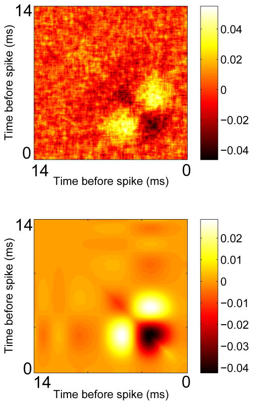
As an illustration, we apply the idea to the HH model. We compute the STA using a fraction of the spikes we need to compute the STC, and then use the above formulas. Figure 10 shows the results of such a computation. Clearly, it works quite well for the HH equations, where 15,000 spikes were computed.

Fig. 10.

Direct approximation of the STC from the STA for the HH equations. (A) Computation of the STC by simulation of the model; (B) Using equations (8)–(10), we approximate the STC.

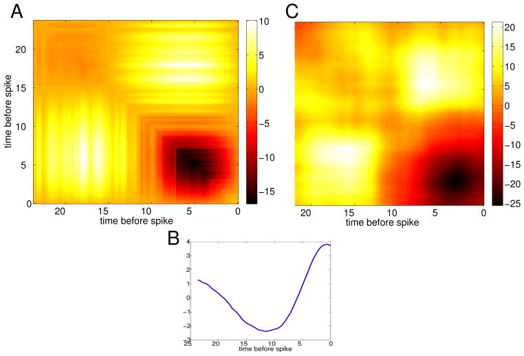
We also looked to see if this method works for real neural data. We obtained data that was used in [17]. A mouse olfactory bulb mitral cell was driven with DC current on top of which was added a small filtered white noise signal. The cell had a frequency of close to 40 Hz and the interspike interval (ISI) coefficient of variation was 0.2. 2526 spikes were collected. Figure 11 shows an example of the application of equation (10) to this data. While the reconstruction is not perfect, most of the features are quite similar with a negative region at early times near the diagonal and two large positive bands off the diagonal.

Fig. 11.

Construction of the STC from the STA for an experimental recording of an olfactory bulb mitral cell. (A) Reconstructed STC using equation (10) and the STA shown in (B). (C) Actual STC computed directly from the data.

4 Discussion

In this paper, we have shown the relationship between the PRC of a neuron and the STC. The method assumes that the stimulus that is driving the neuron is small in amplitude and that the underlying dynamics are oscillatory. While this is somewhat restrictive, the results are very general and provide a direct link between dynamics (the PRC) and coding (STC, STA) of neurons. We have also used this relationship to suggest a direct relationship between the STA and the STC through equation (10). We applied this with good success to a model and with more limited success to a real neuron.

We have shown, somewhat to our surprise, that the main reason that spike frequency adaptation alters the STC is that it introduces a skew to the PRC rather than making it negative and changing it from type I to type II. We nevertheless found that the features to which certain simple classes of phase model neurons are sensitive, shift to earlier times in the cycle (see Figure 8B) as the neuron transitions from a type II PRC (Δ(θ) = − sin θ) to a type I PRC (Δ(θ) = 1 − cos θ). Our spectral results differ from many of the results presented in [8] who also studied differences between type I and II neurons, but for irregularly firing neurons in the strong noise regime. Specifically, we consistently observe bimodality in the first eigenvector for oscillating neurons with parametric type I (Fig. 9) and II dynamics (Fig. 8), while [8] observed predominantly positive, unimodal first eigenvectors for irregularly firing type I neurons. In the low noise, oscillatory regime, however, [8] did observe bimodality in the first eigenvector for a type I neuron, supporting our current results.

Using a stochastic spike response model, [32] analytically confirmed that the modality of a type I neurons STA depends on the strength of input noise. Counter to the results presented here and supported by [8], however, [32] found that reducing the strength of input noise yields unimodal, positive STAs, while strong noise regimes produce bimodal STAs, for one specific type I response kernel. This discrepancy may arise from only considering the first passage time (i.e., the first spike time) in their derivations, while here we restrict our analysis solely to the low noise, oscillatory regime. Indeed, results of [32] and [8] coincide for irregular firing regimes.

What do our results say about neural coding? Adaptation is something that is readily controllable through modulation of certain potassium currents. Thus, we have studied the effects of adaptation on the spectral properties of the STC. Levels of adaptation greater than g = 0.5 shrink the envelope of stimulus-responsiveness for a neuron. In other words, the STC and corresponding eigenvectors are temporally compact for g > 0.5. Thus, spiking in neurons with g > 0.5 would convey less information about early and late phases of the stimulus preceding each spike. Increasing adaptation has two consequences on neural coding from an information theoretic perspective: (i) for g < 1, increasing adaptation reduces the amount of information periodic spiking conveys about the stimulus; (ii) for g > 1, increasing adaptation leads to bimodal PRCs and greater propensity for oscillating neurons to synchronize, thereby reducing population information content but increasing information propagation/fidelity.

There are several places where the theory will break down or needs to be extended. The simple formulae obtained are a result of letting the noise stimulus be white. However, there is no reason why any type of Gaussian process could not also be used, though the formulae become much more complicated. For example, the STA is no longer just the derivative of the PRC but requires convolving it with the autocorrelation function of the stimulus. Since the latter is known, presumably, this is just a simple convolution to perform numerically. Similarly, the direct computation of the STC from the STA is not simple as, again, with colored noise, the relationship would involve both deconvolution and convolution. The former is fraught with numerical issues. In spite of these issues, the theory does provide an exact relationship, even for nonwhite stimuli.

The perturbation theory is exact (in the sense that all terms are accounted for) for weakly perturbed phase models, θ′ = 1 + εξ(t)Δ(θ). However, for real neurons and biophysical models of neurons, there is no phase model. Rather, the phase model is derived from the full model through successive changes of variables, and the result is of the order ε truncation. But, in order to get the STC, we need to go to order ε². For the phase model, there are no ε² terms, so this is not an issue. However, if we start with a neuron or a full biophysical model, then we need to include the higher order terms. These are non-trivial to obtain, even in the simplest oscillator models, and for real neurons are probably impossible to obtain (unlike the PRC, for which there are many experimentally accessible methods [30]). Thus, the theory should be viewed as ignoring possibly important terms when trying to compare it to a full biophysical model and a real neuron. Nevertheless, the HH example (where we started with the full model) seems to indicate that whatever these extra terms, they may not always be important as there is excellent agreement between the full and the phase-reduced model. One possible reason for this is that the order ε² terms for the phase reduction will be very small if the attraction to the limit cycle is strong (see [31]).

Finally, the most important caveat is that the stimuli must be small enough so that the neuron remains close to the limit cycle oscillation. In other words, the coefficient of variation of the ISI should be small. Furthermore, the oscillation should be intrinsic rather than noise driven. This weak stimulus assumption is quite restrictive but it is hard to imagine any general theory that does not make it. By using certain reduced models, [9] have begun to relate dynamics to the STC and STA when stimuli are not weak, but their work requires a linear response up to the spiking threshold.

In sum, we have used the theoretical relationship between the PRC and the STC to connect the intrinsic dynamics of oscillatory neurons to their feature selection.

5 Appendix I

In [33], we show that a neural oscillator driven by weak noise has the form

$$\frac{d\theta }{dt}=1+\epsilon \xi (t)\mathit{\Delta }(\theta (t)),\theta (0)=0,$$ (11)

where θ(t) is the phase of the oscillator, Δ(θ) is the PRC, and ξ(t) is the noisy signal. We will derive formulae for general ξ(t) but will then use white noise (zero mean, δ correlated) for the final results which are compared in the main text. The parameter ε is the amplitude of the noise and is assumed to be small. Indeed, the valid reduction to phase models implicitly assumes that the stimuli are small in magnitude. In order to simplify the analysis, we assume that Δ(0) = 0. This is generally a reasonable assumption and says that the neuron is insensitive to stimuli at the moment it is spiking. Many neural models have this property as do many real neurons. We set θ = 0 to be the phase at which the neuron spikes. If we suppose that θ(0) = 0 (that is, the neuron has spike at t = 0), we want to know at what time the neuron spikes again, t_sp. Since the neuron spikes when θ(t_sp) = T, we must solve (11) to determine t_sp. This was done for small ε in [14]:

$$\begin{array}{l}{t}_{sp}=T+\epsilon {\tau }_1+{\epsilon }^2{\tau }_2\\ {\tau }_1=-{\int }_0^T\xi (s)\mathit{\Delta }(s)ds\\ {\tau }_2=-{\int }_0^T\xi (s){\mathit{\Delta }}^{\prime }(s){\int }_0^s\mathit{\Delta }(s^{\prime })\xi (s^{\prime })d{s}^{\prime }ds.\end{array}$$ (12)

t_sp is a function of the PRC, its derivative, and the noise, ξ(t). The STA and STC are related to moments of the stimulus conditioned on a spike. The stimulus, here, is εξ(t). Thus:

$$\text{STA}(t):=\epsilon {\langle \xi (t_{sp}-t)\rangle }_{t_{sp}}$$ (13)

$$\text{STA}(t_1,t_2):={\epsilon }^2{\langle \xi (t_{sp}-t_1)\xi (t_{sp}-t_2)\rangle }_{t_{sp}}-\text{STA}(t_1)\text{STA}(t_2).$$ (14)

Here, the average is performed over all spikes. However, at each spike the neural oscillator is reset to phase zero, so that we just have to average over all instances of the stimulus, ξ(t). To clarify this, we will use 〈·〉_tsp to indicate average over spike times and 〈·〉 (without the subscript t_sp) to indicate average over the stimulus ξ.

Let C(t) be the autocorrelation for the stimulus. In the STA calculation, we only need to compute τ₁ as we now illustrate:

$$\begin{array}{l}{\langle \epsilon \xi (t_{sp}-t)\rangle }_{t_{sp}}=\epsilon \langle \xi (T+\epsilon {\tau }_1-t)\rangle \\ =\epsilon \langle \xi (T-t)\rangle +{\epsilon }^2\langle {\xi }^{\prime }(T-t){\tau }_1\rangle +O\langle {\epsilon }^2\rangle \\ =-{\epsilon }^2{\int }_0^T\mathit{\Delta }(s)\langle {\xi }^{\prime }(T-t)\xi (s)\rangle ds\\ =-{\epsilon }^2{\int }_0^T\mathit{\Delta }(s)C^{\prime }(T-t-s)ds\\ =-{\epsilon }^2{\int }_0^T{\mathit{\Delta }}^{\prime }(s)C(T-t-s)ds.\end{array}$$

The last step (and many of the subsequent steps in the next few paragraphs) is an application of integration by parts. Finally, if C(t) is a delta function (white noise case), we obtain the known result

$$\text{STA}(t)=-{\epsilon }^2{\mathit{\Delta }}^{\prime }(T-t).$$ (15)

5.1 Covariance

To evaluate the covariance, we need to use higher order terms in the calculation of the spike time, t_sp. Before proceeding with this, we want to address an important caveat. The phase reduction is an order ε approximation to the dynamics of the full model. The use of white noise gives an ε² magnitude for the STA. To get the STC requires that we go to order ε⁴ and so we have expanded the spike time, t_sp out to order ε². However, this is technically not complete since, the phase reduction gives us order ε but we need order ε². For general neural models, computing the order ε² terms (called higher order averaging in the dynamical systems literature) is very difficult. Thus, we have not computed this higher order correction even though it is formally required. In spite of this apparent flaw in our perturbations, we find (as can be seen in the results for the HH model) that the neglect of these additional higher order terms does not seem to hurt our approximation. If we stick to pure phase models and ignore the fact that these models arise from real biophysical oscillators, then the model is precisely equation (11) and the subsequent calculations are correct. However, if we want to compare the results to the full nonlinear oscillator, we must regard this calculation as an approximation only.

For simplicity, we first factor out the ε² in the definition of the STC. We next state a few identities for the moments of Gaussian processes that we need for the calculations below:

$$\begin{array}{l}\langle {\xi }_1(t_1){\xi }_2(t_2){\xi }_3(t_3)\rangle =0\\ \langle {\xi }_1(t_1){\xi }_2(t_2){\xi }_3(t_3){\xi }_4(t_4)\rangle =\langle {\xi }_1(t_1){\xi }_2(t_2)\rangle \langle {\xi }_3(t_3){\xi }_4(t_4)\rangle +\langle {\xi }_1(t_1){\xi }_3(t_3)\rangle \langle {\xi }_2(t_2){\xi }_4(t_4)\rangle +\langle {\xi }_1(t_1){\xi }_4(t_4)\rangle \langle {\xi }_2(t_2){\xi }_3(t_3)\rangle \\ \langle {\xi }^{\prime }(t)\xi (s)\rangle =C^{\prime }(t-s)=-C^{\prime }(s-t)\\ \langle {\xi }^{″}(t)\xi (s)\rangle =C^{″}(t-s)=C^{″}(s-t)\\ \langle {\xi }^{\prime }(t){\xi }^{\prime }(s)\rangle =-C^{″}(t-s)=-C^{″}(s-t)\end{array}$$ (16)

The first two are given in the Appendix of [3] and the rest follow from the definitions of the autocorrelation function. We will formally write derivatives of ξ(t), but as we will be averaging and integrating these quantities with respect to smooth functions, we can think of these manipulations in the sense of distributions.

We expand ξ(t_sp − t_j) (j = 1, 2). Since the i^th spike is given by the formula (12), we obtain:

$$\xi (T-t_j+\epsilon {\tau }_1+{\epsilon }^2{\tau }_2)=\xi (T-t_j)+\epsilon {\xi }^{\prime }(T-t_j){\tau }_1+{\epsilon }^2[{\xi }^{\prime }(T-t_j){\tau }_2+(1/2){\xi }^{″}(T-t_j){\tau }_1^2]+\dots$$

We multiply ξ(t_spike − t₁) ξ(t_spike − t₂) and keep up to order ε²:

$$\begin{array}{l}\xi (t_{\mathit{spike}}-t_1)\xi (t_{\mathit{spike}}-t_2)=\xi (T-t_1)\xi (T-t_2)\\ +\epsilon {\tau }_1[\xi (T-t_1){\xi }^{\prime }(T-t_2)+\xi (T-t_2){\xi }^{\prime }(T-t_1)]\\ +{\epsilon }^2{\tau }_1^2/2[\xi (T-t_1){\xi }^{″}(T-t_2)+\xi (T-t_2){\xi }^{″}(T-t_1)]\\ +{\epsilon }^2{\tau }_1^2{\xi }^{\prime }(T-t_1){\xi }^{\prime }(T-t_2)\\ +{\epsilon }^2{\tau }_2[\xi (T-t_1){\xi }^{\prime }(T-t_2)+\xi (T-t_2){\xi }^{\prime }(T-t_1)]\end{array}$$

We now average this over all spikes (instances of ξ) to get the expected value of the product. The order 1 term (first line) is the stimulus correlation C(t₂ − t₁). The order ε terms consist of products of ξ and its derivative and τ, which, itself contains a ξ, hence there order ε terms consist of averages of triples of ξ(t). According to the first identity in equation (16), the average of these triplets is zero, so there are no order ε terms. However, ${\tau }_1^2$ and τ₂ both contain terms with ξ(t) appearing as a product. Specifically:

$$\begin{array}{l}{\tau }_1^2={\int }_0^T{\int }_0^T\mathit{\Delta }(s)\mathit{\Delta }(s^{\prime })\xi (s)\xi (s^{\prime })d{s}^{\prime }ds\\ {\tau }_2={\int }_0^T{\int }_0^s{\mathit{\Delta }}^{\prime }(s)\mathit{\Delta }(s^{\prime })\xi (s)\xi (s^{\prime })d{s}^{\prime }ds.\end{array}$$

Thus, when we average over the noisy process, we will get products of four different variants of ξ(t) so that we can use the identities in (16) to evaluate these.

We do the ${\tau }_1^2$ terms first. We must evaluate the following average:

$$\begin{array}{l}{A}_1(t_1,t_2):={\int }_0^T{\int }_0^T\mathit{\Delta }(s)\mathit{\Delta }(s^{\prime })\langle \xi (s)\xi (s^{\prime })[\xi (T-t_1){\xi }^{″}(T-t_2)+\xi (T-t_2){\xi }^{″}(T-t_1)]\rangle d{s}^{\prime }ds\\ +{\int }_0^T{\int }_0^T\mathit{\Delta }(s)\mathit{\Delta }(s^{\prime })\langle \xi (s)\xi (s^{\prime }){\xi }^{\prime }(T-t_1){\xi }^{\prime }(T-t_2)\rangle d{s}^{\prime }ds\end{array}$$

We need to evaluate:

$$M_1(t_1,t_2,s,s^{\prime }):=\langle ({\xi }^{\prime }(T-t_1){\xi }^{\prime }(T-t_2)\xi (s)\xi (s^{\prime })\rangle +\frac{1}{2}\langle ({\xi }^{″}(T-t_1)\xi (T-t_2)\xi (s)\xi (s^{\prime })\rangle +\frac{1}{2}\langle ({\xi }^{″}(T-t_2)\xi (T-t_1)\xi (s)\xi (s^{\prime })\rangle$$

which, using the identities (16), becomes

$$\begin{array}{l}{M}_1(t_1,t_2,s,s^{\prime })=C^{\prime }(t_1+s-T)C^{\prime }(t_2+s^{\prime }-T)+C^{\prime }(s^{\prime }+t_1-T)C^{\prime }(s+t_2-T)\\ +\frac{1}{2}{C}^{″}(t_1+s-T)C(s^{\prime }+t_2-T)+\frac{1}{2}{C}^{″}(t_1+s^{\prime }-T)C(s+t_2-T)\\ +\frac{1}{2}{C}^{″}(t_2+s-T)C(s^{\prime }+t_1-T)+\frac{1}{2}{C}^{″}(t_2+s^{\prime }-T)C(s+t_1-T)\end{array}$$

(Note that there are terms of the form C″(t₂ − t₁)C(s − s′) which would be very troublesome, but, they are canceled out with the same pair with opposite signs.) We now integrate M₁ with the PRCs and assume the noise is white so we can evaluate the integrals:

$$\begin{array}{l}{A}_1(t_1,t_2)={\int }_0^T{\int }_0^T\mathit{\Delta }(s)\mathit{\Delta }(s^{\prime })M_1(t_1,t_2,s,s^{\prime })d{s}^{\prime }ds\\ =2{\mathit{\Delta }}^{\prime }(T-t_2){\mathit{\Delta }}^{\prime }(T-t_1)+{\mathit{\Delta }}^{″}(T-t_2)\mathit{\Delta }(T-t_1)+{\mathit{\Delta }}^{″}(T-t_1)\mathit{\Delta }(T-t_2),\end{array}$$

where we have again used integration by parts to take care of the derivatives of the correlation function (which are derivatives of delta functions).

This is the easy part because the integrals are all definite and over the periodic domain. We now turn to the τ₂ integrals. We must evaluate this average:

$$A_2(t_1,t_2):=-{\int }_0^T{\int }_0^s{\mathit{\Delta }}^{\prime }(s)\mathit{\Delta }(s^{\prime })\langle (\xi (T-t_1){\xi }^{\prime }(T-t_2)+\xi (T-t_2){\xi }^{\prime }(T-t_1))\xi (s)\xi (s^{\prime })\rangle d{s}^{\prime }ds$$

Let

$$M_2(t_1,t_2,s,s^{\prime }):=\langle (\xi (T-t_1){\xi }^{\prime }(T-t_2)+\xi (T-t_2){\xi }^{\prime }(T-t_1))\xi (s)\xi (s^{\prime })\rangle$$

Then using the identities, (16), we get

$$\begin{array}{l}{M}_2(t_1,t_2,s,s^{\prime })=-C(s+t_1-T)C^{\prime }(t_2+s^{\prime }-T)-C(s^{\prime }+t_1-T)C^{\prime }(t_2+s-T)\\ +-C(s+t_2-T)C^{\prime }(t_1+s^{\prime }-T)-C(s^{\prime }+t_2-T)C^{\prime }(t_1+s-T).\end{array}$$

Consider the following integral

$$I_1:={\int }_0^T{\mathit{\Delta }}^{\prime }(s)C(s+t_2-T){\int }_0^s\mathit{\Delta }(s^{\prime })C^{\prime }(t_1+s^{\prime }-T)d{s}^{\prime }ds.$$

Integrate the inner integral by parts to get:

$${\int }_0^s\mathit{\Delta }(s^{\prime })C^{\prime }(t_1+s^{\prime }-T)d{s}^{\prime }=\mathit{\Delta }(s)C(t_1-s-T)-{\int }_0^s{\mathit{\Delta }}^{\prime }(s^{\prime })C(t_1+s^{\prime }-T)d{s}^{\prime }$$

This means that

$$I_1=-{\int }_0^T{\mathit{\Delta }}^{\prime }(s)C(s+t_2-T){\int }_0^s{\mathit{\Delta }}^{\prime }(s^{\prime })C(t_1+s^{\prime }-T)d{s}^{\prime }ds+{\int }_0^T{\mathit{\Delta }}^{\prime }(s)\mathit{\Delta }(s)C(s+t_2-T)C(s+t_1-T)ds.$$

We will as above, assume that C(s) is a delta function. Let us deal with the first part of the integral. If T − t₁ > s then the integral vanishes since the point of concentration of the delta function is not in the interval of integration. On the other hand, if the inequality is reversed, then the integral is just Δ′(T − t₁) So we can write the first integral as

$$-{\int }_0^{T}C(s+t_2-T){\mathit{\Delta }}^{\prime }(s){\mathit{\Delta }}^{\prime }(T-t_1)H_0(s-T+t_1)ds$$

and we can thus evaluate this to be

$$-{\mathit{\Delta }}^{\prime }(T-t_2){\mathit{\Delta }}^{\prime }(T-t_1)H_0(t_1-t_2).$$

We note that H₀(t) is the usual Heaviside step function with the additional property that H₀(0) = 1/2. The second part is also a bit tricky. If C(s) is a delta function, then this integral is zero unless t₁ = t₂ in which case it is a delta function, Δ′(T − t₁)Δ(T − t₂)C(t₂ − t₁). Thus

$$I_1=-{\mathit{\Delta }}^{\prime }(T-t_2){\mathit{\Delta }}^{\prime }(T-t_1)H_0(t_1-t_2)+{\mathit{\Delta }}^{\prime }(T-t_1)\mathit{\Delta }(T-t_2)C(t_2-t_1).$$

(We keep the C in the expression rather than replacing it with a delta function because when we compare to simulations, this will be a finite large quantity rather than a delta function.)

We can similarly evaluate

$$I_2:={\int }_0^T{\mathit{\Delta }}^{\prime }(s)C(s+t_1-T){\int }_0^s\mathit{\Delta }(s^{\prime })C^{\prime }(t_2+s^{\prime }-T)d{s}^{\prime }ds.$$

as

$$I_2=-{\mathit{\Delta }}^{\prime }(T-t_1){\mathit{\Delta }}^{\prime }(T-t_2)H_0(t_2-t_1)+{\mathit{\Delta }}^{\prime }(T-t_2)\mathit{\Delta }(T-t_1)C(t_1-t_2).$$

The sum of these two integrals is thus

$$I_1+I_2=(2C(t_2-t_1)-1){\mathit{\Delta }}^{\prime }(T-t_1){\mathit{\Delta }}^{\prime }(T-t_2).$$

We are now left with two integrals. The first is

$$I_3:={\int }_0^T{\mathit{\Delta }}^{\prime }(s)C^{\prime }(t_1+s-T){\int }_0^s\mathit{\Delta }(s^{\prime })C(t_2+s^{\prime }-T)d{s}^{\prime }ds.$$

Using the same logical approach (we need s > T − t₂) and an integration by parts on the outer integral, we get

$$I_3:=-{\mathit{\Delta }}^{″}(T-t_1)\mathit{\Delta }(T-t_2)H_0(t_2-t_1).$$

Finally, (by switching indices) the last integral is

$$I_4:={\mathit{\Delta }}^{″}(T-t_2)\mathit{\Delta }(T-t_1)H_0(t_1-t_2).$$

Summing A₁ + A₂ and subtracting off the product of the means we obtain the desired formula for the covariance (t₂ ≠ t₁):

$$\begin{array}{l}\text{STC}(t_1,t_2)={\epsilon }^{2}C(t_2-t_1)+{\epsilon }^4[{\mathit{\Delta }}^{″}(T-t_2)\mathit{\Delta }(T-t_1)(1-H_0(t_1-t_2))+{\mathit{\Delta }}^{″}(T-t_1)\mathit{\Delta }(T-t_2)(1-H_0(t_2-t_1))]\\ ={\epsilon }^{2}C(t_2-t_1)+{\epsilon }^4[{\mathit{\Delta }}^{″}(T-t_2)\mathit{\Delta }(T-t_1)H_0(t_2-t_1)+{\mathit{\Delta }}^{″}(T-t_1)\mathit{\Delta }(T-t_2)H_0(t_1-t_2)].\end{array}$$

References

- 1.Bryant H, Segundo J. The Journal of physiology. 1976;260(2):279. doi: 10.1113/jphysiol.1976.sp011516. [DOI] [PMC free article] [PubMed] [Google Scholar]
- 2.Marmarelis P, Marmarelis V. Analysis of physiological systems: The white-noise approach. Plenum Press; New York: 1978. [Google Scholar]
- 3.Rieke F, Warland D, DeRuyter van Steveninck R, Bialek W. Spikes: exploring the neural code (computational neuroscience) The MIT Press; 1999. [Google Scholar]
- 4.Arcas B, Fairhall A. Neural Computation. 2003;15(8):1789. doi: 10.1162/08997660360675044. [DOI] [PubMed] [Google Scholar]
- 5.Arcas B, Fairhall A, Bialek W. Neural Computation. 2003;15(8):1715. doi: 10.1162/08997660360675017. [DOI] [PubMed] [Google Scholar]
- 6.Schwartz O, Pillow J, Rust N, Simoncelli E. Journal of Vision. 2006;6(4) doi: 10.1167/6.4.13. [DOI] [PubMed] [Google Scholar]
- 7.Dayan P, Abbott L, Abbott L. Theoretical neuroscience: Computational and mathematical modeling of neural systems. Taylor & Francis; 2001. [Google Scholar]
- 8.Mato G, Samengo I. Neural computation. 2008;20(10):2418. doi: 10.1162/neco.2008.10-07-632. [DOI] [PubMed] [Google Scholar]
- 9.Famulare M, Fairhall A. Neural computation. 2010;22(3):581. doi: 10.1162/neco.2009.02-09-956. [DOI] [PubMed] [Google Scholar]
- 10.Izhikevich E. Dynamical systems in neuroscience: the geometry of excitability and bursting. The MIT press; 2007. [Google Scholar]
- 11.Paninski L. Neural computation. 2006;18(11):2592. doi: 10.1162/neco.2006.18.11.2592. [DOI] [PubMed] [Google Scholar]
- 12.Hong S, Agüera y Arcas B, Fairhall A. Neural computation. 2007;19(12):3133. doi: 10.1162/neco.2007.19.12.3133. [DOI] [PubMed] [Google Scholar]
- 13.Ostojic S, Brunel N. PLoS Computational Biology. 2011;7(1):e1001056. doi: 10.1371/journal.pcbi.1001056. [DOI] [PMC free article] [PubMed] [Google Scholar]
- 14.Ermentrout G, Galán R, Urban N. Physical review letters. 2007;99(24):248103. doi: 10.1103/PhysRevLett.99.248103. [DOI] [PMC free article] [PubMed] [Google Scholar]
- 15.Marella S, Ermentrout G. Physical review E. 2008;77(4):041918. doi: 10.1103/PhysRevE.77.041918. [DOI] [PubMed] [Google Scholar]
- 16.Abouzeid A, Ermentrout B. Physical Review E. 2011;84(6):061914. doi: 10.1103/PhysRevE.84.061914. [DOI] [PubMed] [Google Scholar]
- 17.Burton S, Ermentrout G, Urban N. Journal of Neurophysiology. 2012 doi: 10.1152/jn.00362.2012. [DOI] [PMC free article] [PubMed] [Google Scholar]
- 18.Gutkin B, Ermentrout G, Reyes A. Journal of neurophysiology. 2005;94(2):1623. doi: 10.1152/jn.00359.2004. [DOI] [PubMed] [Google Scholar]
- 19.Kuramoto Y. Chemical oscillations, waves, and turbulence. Dover Pubns; 2003. [Google Scholar]
- 20.Ermentrout G, Terman D. Mathematical foundations of neuroscience. Vol. 35. Springer Verlag; 2010. [Google Scholar]
- 21.Ermentrout B. Simulating, analyzing, and animating dynamical systems: a guide to XPPAUT for researchers and students. Vol. 14. Society for Industrial Mathematics; 2002. [Google Scholar]
- 22.Barreiro A, Shea-Brown E, Thilo E. Physical Review E. 2010;81(1):011916. doi: 10.1103/PhysRevE.81.011916. [DOI] [PubMed] [Google Scholar]
- 23.Ota K, Omori T, Watanabe S, Miyakawa H, Okada M, Aonishi T. BMC Neuroscience. 2010;11(Suppl 1):P14. [Google Scholar]
- 24.Brown E, Moehlis J, Holmes P. Neural Computation. 2004;16(4):673. doi: 10.1162/089976604322860668. [DOI] [PubMed] [Google Scholar]
- 25.Galán R, Bard Ermentrout G, Urban N. Neurocomputing. 2007;70(10):2102. [Google Scholar]
- 26.Hansel D, Mato G, Meunier C. Neural Computation. 1995;7(2):307. doi: 10.1162/neco.1995.7.2.307. [DOI] [PubMed] [Google Scholar]
- 27.Ermentrout B, Pascal M, Gutkin B. Neural Computation. 2001;13(6):1285. doi: 10.1162/08997660152002861. [DOI] [PubMed] [Google Scholar]
- 28.Pfeuty B, Mato G, Golomb D, Hansel D. The Journal of neuroscience. 2003;23(15):6280. doi: 10.1523/JNEUROSCI.23-15-06280.2003. [DOI] [PMC free article] [PubMed] [Google Scholar]
- 29.Ermentrout G, Beverlin B, Netoff T. Phase Response Curves in Neuroscience. 2012:207–236. [Google Scholar]
- 30.Torben-Nielsen B, Uusisaari M, Stiefel K. Frontiers in neuroinformatics. 2010;4 doi: 10.3389/fninf.2010.00006. [DOI] [PMC free article] [PubMed] [Google Scholar]
- 31.Ermentrout G, Kopell N. Journal of Mathematical Biology. 1991;29(3):195. [Google Scholar]
- 32.Omori T, Aonishi T, Okada M. Physical Review E. 2010;81(2):021901. doi: 10.1103/PhysRevE.81.021901. [DOI] [PubMed] [Google Scholar]
- 33.Teramae J, Nakao H, Ermentrout G. Physical review letters. 2009;102(19):194102. doi: 10.1103/PhysRevLett.102.194102. [DOI] [PubMed] [Google Scholar]