A Bayesian framework for simultaneously modeling neural and behavioral data

Abstract

Scientists who study cognition infer underlying processes either by observing behavior (e.g., response times, percentage correct) or by observing neural activity (e.g., the BOLD response). These two types of observations have traditionally supported two separate lines of study. The first is led by cognitive modelers, who rely on behavior alone to support their computational theories. The second is led by cognitive neuroimagers, who rely on statistical models to link patterns of neural activity to experimental manipulations, often without any attempt to make a direct connection to an explicit computational theory. Here we present a flexible Bayesian framework for combining neural and cognitive models. Joining neuroimaging and computational modeling in a single hierarchical framework allows the neural data to influence the parameters of the cognitive model and allows behavioral data, even in the absence of neural data, to constrain the neural model. Critically, our Bayesian approach can reveal interactions between behavioral and neural parameters, and hence between neural activity and cognitive mechanisms. We demonstrate the utility of our approach with applications to simulated fMRI data with a recognition model and to diffusion-weighted imaging data with a response time model of perceptual choice.

Introduction

Currently, there are two main methods to study cognition. The first and oldest method is known as cognitive modeling. Given a set of experimental data, one assumes that observers use a particular process, known as a cognitive model, to produce the observed data. The processes used by the cognitive model are controlled by a set of unknown parameters. The parameters of the cognitive model are then estimated and psychologically meaningful interpretations are based on these parameter estimates. While cognitive models have been effective tools for identifying how cognition changes as a function of task demands, they suffer from being highly abstract representations of what is essentially a system of biological processes. The second method to study cognition is to make contact with the biological substrate more directly and measure brain activity using methods such as positron emission tomography (PET), functional-magnetic resonance imaging (fMRI), electroencephalography (EEG), or diffusion-weighted imaging (DWI), and we will refer to this broad class of data as “neural data”. While neural data provide valuable information about the biological and physical aspects of cognition, traditional neural imaging analyses (e.g., general linear models) are limited because they do not attempt to describe cognitive processes. Because both methods for studying cognition have clear advantages and disadvantages (Wilkinson and Halligan, 2004), there has been a recent surge of interest in combining both sources of information to provide a single explanation of the underlying process (e.g., Anderson et al., 2008; Borst et al., 2011; Dolan, 2008; Forstmann et al., 2008, 2010, 2011; Gläscher and O'Doherty, 2010; O'Doherty et al., 2007).

In this article, we propose a general framework for describing neural and behavioral data with a single model. Our approach is to treat the two sources of information as separate measurements of the same cognitive construct. To fit the model, we make use of a hierarchical Bayesian approach, which has become an important method for inference in both the neural (e.g., Friston et al., 2002; Gershman et al., 2011; Guo et al., 2008; Wu et al., 2011), and cognitive modeling (e.g., Lee, 2011; Shiffrin et al., 2008) literatures.

Using the hierarchical Bayesian approach provides a number of benefits. First, the Bayesian framework provides meaningful, interpretable information at both the subject and group levels. Second, the Bayesian framework lends itself naturally to principled inclusion of missing data. We will show how our framework allows us to make predictions for missing data, based solely on parameter relationships learned from fitting the model. In particular, we show that we can make informed predictions of behavioral data given only neural data, and vice versa. Third, our framework allows us to infer relationships between parameters, relationships that need not be hypothesized a priori. This feature affords us explorative opportunities in the form of the Bayesian posterior distribution. Fourth, the framework we propose does not require a commitment to any particular model, as in other joint modeling approaches (e.g., Anderson et al., 2008; Borst et al., 2011; Mazurek et al., 2003). By using a hierarchical Bayesian approach, we can choose any particular cognitive model to explain the behavioral data, and any neural model to explain the neural data. Subsequently, our framework links the two models together and simultaneously infers meaningful relationships between the two models while also providing a unifying account of brain and behavioral data.

Using such a framework also provides a method for answering much more general questions, which we do not attempt to answer here. For example, linking brain and behavioral data allows us to directly perform model selection on multiple theories of cognition. One could fit several different cognitive models combined with a single neural model to data, and the joint model that fit the full data set best would be the preferred model. In this way, the neural data provides deeper constraints on cognitive models, and in so doing, can be used to better test cognitive theories.

We first provide a brief introduction to the two different types of measurements, and then describe our joint modeling approach. We then demonstrate the utility of our approach in a simulation study. Finally, we apply our model to data from an experiment containing both neural data and behavioral data that can be fit with a computational model. We show that meaningful relationships between model parameters and neural data can be inferred directly from fitting the model, and these relationships can be further exploited to make predictions about the distribution of missing or unobserved data.

Prior research

Although both behavioral and neural data are central to the study of cognition, few attempts have been made to merge them. Perhaps one of the most successful approaches toward this goal is model-based fMRI analysis (Gläscher and O'Doherty, 2010; O'Doherty et al., 2007). In this procedure, a cognitive model is first used to simulate neural data. To do this, often cognitive models are convolved with particular functions that resemble neural effects, such as the hemodynamic response function that resembles the blood oxygen level dependent (BOLD) response (e.g., Anderson et al., 2008). The simulated neural data are then compared with the observed neural data by means of a correlation analysis. Because the approach is not limited exclusively to fMRI data, we will refer to the approach as “model-based neural analysis.” The method has been successful in identifying areas of the brain involved in reinforcement learning (e.g., O'Doherty et al., 2003, 2007), abstract learning (Hampton et al., 2006), and symbolic processing (Borst and Anderson, 2012; Borst et al., 2011). Despite the method's success, model-based neural analyses uncover meaningful relationships only after individual analyses of both the neural and behavioral data have been performed. As a result, the information contained in the neural data does not constrain the parameters of the cognitive model — it only serves to either support or refute the assumptions made by the cognitive model.

Other approaches aim to incorporate mechanisms that describe the production of neural data into the cognitive model (e.g., Anderson et al., 2007, 2008, 2010, 2012; Fincham et al., 2010; Mazurek et al., 2003). As an example, Anderson et al. (2008) developed a model of the process of equation solving within the ACT-R architecture (Anderson, 2007). The ACT-R model assumed that observers manage a set of modules that activate and deactivate to perform certain operations. For example, the visual module is active initially to encode the stimulus and may also be active when a response is elicited (e.g., a saccade), but it is inactive at certain times within the trial. The various modules are all mapped to different regions of the brain (see Anderson et al., 2007), and each region of the brain becomes active in tandem with the corresponding module. To produce the BOLD response, Anderson et al. (2008) convolved a binary module activation function (i.e., either inactive or active) with a hemodynamic response function. The model was shown to provide a reasonable fit to both the neural and behavioral data.

The problem with designing an architecture that connects specific brain regions to the mechanisms used by a cognitive model is two-fold. First, identifying which region(s) of the brain should be connected to which mechanism(s) of the cognitive model (e.g., modules in ACT-R) is a difficult task. Not only would it require a substantial amount of prior research, but the mechanisms assumed by the model may not be neurologically plausible, and so they will not map directly to any particular brain region or brain regions. Second, while the model can inform specific hypotheses of interest, it is unable to provide information that does not conform to a specific a priori hypothesis (O'Doherty et al., 2007).

The linear ballistic accumulator (LBA; Brown and Heathcote, 2008) model is an example of a model whose mechanisms do not yet have clear mappings to brain regions. While we will delay a detailed discussion until later, the LBA is a model of choice response time (RT) that has recently been used to further our understanding of how biological properties of the brain affect behavioral data (Forstmann et al., 2008, 2010, 2011). For example, Forstmann et al. (2008) performed a speed–accuracy experiment with two conditions of task demands. In the first condition, subjects were told to respond accurately, and in the second condition, subjects were asked to respond quickly. In addition to obtaining choice and RT data, Forstmann et al. examined fMRI data during each condition. In a contrast analysis on the neural data, Forstmann et al. determined that preparation for fast responses (i.e., the speed emphasis condition) involved the anterior striatum and the pre-SMA. Forstmann et al. (2008) then fit the LBA model to the behavioral data. The LBA model generally accounts for faster, more error-prone decisions made by subjects in the speed emphasis condition by decreasing the model parameter that represents the amount of evidence required to make a decision. The idea behind this assertion is that an observer lowers a “threshold” parameter so that they can make decisions faster, but in so doing, they compromise their accuracy by limiting the amount of evidence on which decisions are based.

Once both the neural and behavioral data had been analyzed, Forstmann et al. (2008) examined the correlations between the instruction-induced differences in response caution with instruction-induced differences in the activation of the anterior striatum and the pre-SMA. The relation between the two variables was negative, indicating that subjects who had a relatively large increase in activation in the right anterior striatum and the right pre-SMA also adjusted their response caution parameter more as the instruction-induced pressure to respond quickly increased. Thus, the degree of activation in these two brain areas was linked to the adjustment of the response caution parameter. Other features of the brain have been connected with parameters of the LBA model. For example, Forstmann et al. (2010, 2011) have found evidence suggesting that the flexible adjustment of the response caution parameter under different time pressures is related to the strength of certain corticostriatal white matter connections. Taken together, these results suggest that process models, in this case the LBA model, along with behavioral data can be used to draw conclusions about biological properties of the brain.

While the work of Forstmann et al. (2008, 2010, 2011) has been instrumental in furthering our understanding of how related the LBA model is to actual brain processing and brain structure, these model-based neural analyses can be improved upon. Because the neural and behavioral data are both measuring the same construct (i.e., cognition), it would be ideal if one model could be used to explain both sources of data simultaneously. In this article, we argue that process models should be considerate of biological constraints and physical systems in addition to the cognitive mechanisms they assume.

The framework

We wish to provide a joint explanation for the jth subject's neural N_j and behavioral B_j data. If it is difficult or undesirable to specify the joint distribution of (N_j, B_j) under a single model, we can begin by describing how each individual source should be modeled. We will denote the cognitive model as Behav with unknown parameters θ, and the neural model as Neural with unknown parameters δ. A key benefit of our framework is that we are not limited to a particular cognitive or neural model. For example, we can choose a number of different cognitive models, such as the LBA model (Brown and Heathcote, 2008), the classic model of signal detection theory (Green and Swets, 1966), or the generalized context model (Nosofsky, 1986). Similarly, the neural model may also take a variety of forms, such as the generalized linear model (Frank et al., 1998; Guo et al., 2008; Kershaw et al., 1999), the topographic latent source analysis model (Gershman et al., 2011), a wavelet process (Flandin and Penny, 2007), a dynamic causal model (Friston et al., 2003), or a hemodynamic response function (Friston, 2002). While not essential, neural models can help to reduce the dimensionality of the neural data N_j by summarizing the data with a set of sources of interest. Once the neural data from an experiment have been fit with the neural model, one can make meaningful comparisons between the neural sources across experimental conditions. Regardless of the chosen model pair, we assume that the neural data come from the neural model, so that

$$N_j~\text{Neural}\left({\delta }_j\right),$$

and the behavioral data come from the cognitive model, so that

$$B_j~\text{Behav}\left({\theta }_j\right).$$

With an appropriate explanation of both sources of data in hand, we now combine the parameters of the two models into a single joint model $\mathcal{M}$ of neural and behavioral data. Specifically, we can write this joint model as

$$\left({\delta }_j,{\theta }_j\right)~\mathcal{M}\left(\Omega \right).$$

where Ω denotes the collection of hyperparameters. For example, Ω might consist of a set of hyper mean parameters ϕ and hyper dispersion parameters Σ so that Ω={Φ, Σ}.

To fit the joint model to data, we will use a hierarchical Bayesian approach, which has recently aided many neural analyses (e.g., Gershman et al., 2011; Guo et al., 2008; Kershaw et al., 1999; Quirós et al., 2010; Van Gerven et al., 2010; Wu et al., 2011). Given the above model specification, we can write the joint posterior distribution of the model parameters as

$$\begin{array}{cc}\hfill p(\Omega ,\theta ,\delta \mid N,B)& \propto p\left(\Omega \right)\mathcal{M}\left(\right(\theta ,\delta )\mid \Omega )\text{Behav}(B\mid \theta )\text{Neural}(N\mid \delta )\hfill \\ \hfill & \propto p\left(\Omega \right)\prod _{j=1}^J\left[\mathcal{M}\left(\left({\theta }_j,{\delta }_j\right)\mid \Omega \right)\text{Behav}\left(B_j\mid {\theta }_j\right)\text{Neural}\left(N_j\mid {\delta }_j\right)\right],\hfill \end{array}$$ (1)

where p(·) denotes a probability distribution, Behav(a|b) and Neural(a|b) denote the density functions of the data a given the parameters b under the behavioral and neural model, respectively. Similarly, $\mathcal{M}\left(\right(a,b)\mid c)$ denotes the joint density function of the parameters (a,b) given the parameters c under the joint model.

Fig. 1 shows a graphical diagram for the joint modeling framework. On the left side of the diagram, we have the neural data N_j and the neural model parameters δ_j, whereas on the right side of the diagram we have the behavioral data B_j and the cognitive model parameters θ_j. In the middle of the diagram, we see the hyperparameters ϕ and Σ, which may reflect the central tendency or dispersion parameters of the hyperparameter set Ω={ϕ, Σ}, that connect the two model parameter sets to one another. The subject-specific parameters θ_j and δ_j are conditionally independent given the hyperparameters, but importantly, they are not marginally independent. As we will see later in this article, the dependency between these parameters can be used to mutually constrain the parameter estimates.

Fig. 1.

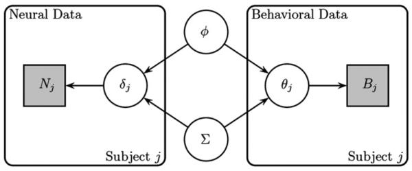
Graphical diagram for the joint modeling approach of neural (left side) and behavioral (right side) data.

The hyperparameters Ω provide an advantage over other modeling approaches. For example, suppose for the jth subject, we were able to obtain only behavioral data, and not neural data. The proposed model would learn about the typical patterns of individual differences from one subject to the next and store this information in the hyperparameters ϕ and Σ. Because we have only subject-specific information in the form of the data B_j, the only subject-specific parameter estimates that can be directly inferred from the data are θ_j. However, the pattern of between-subject variation learned through the hyperparameters is used to form an estimate of a particular subject's neural model parameters δ_j, even when no neural data for Subject j are present. Perhaps more interesting is that we can then use the neural model parameter estimates to make predictions about what the neural data for that subject might have looked like, conditional only on the behavioral data. We will demonstrate this technique in the next section.

A particular instantiation of the joint model

Because both the neural model parameters δ_j and the cognitive model parameters θ_j are intrinsic to the jth subject, our principled approach connects these parameters to one another in a meaningful way. However, to accomplish this, we must make an assumption about the form of the joint distribution of (δ_j,θ_j). In this article, we use a multivariate normal distribution. Thus, we assume that the joint distribution of (δ_j,θ_j) is given by

$$\left({\delta }_j,{\theta }_j\right)~{\mathcal{N}}_p(\varphi ,\Sigma ),$$

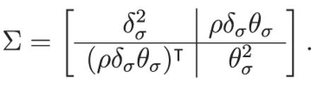
where ${\mathcal{N}}_p(a,b)$ denotes the multivariate normal distribution of dimension p with mean vector a and variance-covariance matrix b. The parameter mean vector ϕ contains all of the group-level mean parameters, so that ϕ={δ_μ,θ_μ} and Σ is the variance–covariance matrix for the group-level variance parameters, namely

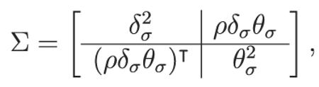where ρ is a matrix containing all of the model parameter correlations that are of interest.

The variance–covariance matrix Σ is partitioned to reflect that it is a mixture of diagonal and full matrices when there are multiple parameters in the neural or behavioral vectors. For example, suppose our neural and cognitive models contain three parameters per subject (i.e., δ_j and θ_j each have three elements). We can then write the partition as

$${\delta }_{\sigma }^2=\left[\begin{array}{ccc}\hfill {\delta }_{\sigma ,1}^2\hfill & \hfill 0\hfill & \hfill 0\hfill \\ \hfill 0\hfill & \hfill {\delta }_{\sigma ,2}^2\hfill & \hfill 0\hfill \\ \hfill 0\hfill & \hfill 0\hfill & \hfill {\delta }_{\sigma ,3}^2\hfill \end{array}\right],$$

where δ_σ,1 denotes the hyper standard deviation for the first model parameter set. We can constrain off-diagonal elements to be zero if we are not interested in quantifying the correlations between a set of model parameters. The relationships between the model parameters will still be inferred by the model because the dependencies exist in the likelihood function. Thus, we can still detect trade-offs that exist between model parameters by examining their joint posterior distribution once the model has been fit to the data. On the other hand, we write the partition that combines the neural and cognitive model parameters as

$$\rho {\delta }_{\sigma }{\theta }_{\sigma }=\left[\begin{array}{ccc}\hfill {\rho }_{11}{\delta }_{\sigma ,1}{\theta }_{\sigma ,1}\hfill & \hfill {\rho }_{12}{\delta }_{\sigma ,1}{\theta }_{\sigma ,2}\hfill & \hfill {\rho }_{13}{\delta }_{\sigma ,1}{\theta }_{\sigma ,3}\hfill \\ \hfill {\rho }_{21}{\delta }_{\sigma ,2}{\theta }_{\sigma ,1}\hfill & \hfill {\rho }_{22}{\delta }_{\sigma ,2}{\theta }_{\sigma ,2}\hfill & \hfill {\rho }_{23}{\delta }_{\sigma ,2}{\theta }_{\sigma ,3}\hfill \\ \hfill {\rho }_{31}{\delta }_{\sigma ,3}{\theta }_{\sigma ,1}\hfill & \hfill {\rho }_{32}{\delta }_{\sigma ,3}{\theta }_{\sigma ,2}\hfill & \hfill {\rho }_{33}{\delta }_{\sigma ,3}{\theta }_{\sigma ,3}\hfill \end{array}\right].$$

Specifying the model in this way allows us to infer directly the degree to which cognitive model parameters are related to which neural model parameters. However, one can also choose to reduce the number of model parameters by constraining some elements of this variance–covariance matrix to be equal to zero (e.g., ρ₃₃=0).

Note that we are not restricted to a multivariate normal distribution in our specification of $\mathcal{M}\left(\Omega \right)$. We chose the multivariate normal because it provides a convenient distribution with infinite support with clear parameter interpretations. For example, the correlation parameters ρ provide a quantification of magnitude and direction of the relationship between pairs of model parameters. Despite this, the use of multivariate normality may not be appropriate in some situations. For example, when the support of a parameter is bounded, it may not be appropriate to assume an infinite support via the normal distribution. However, the multivariate normal distribution can easily be truncated to accommodate various parameter space supports and provides a convenient way to assess the relationship between the neural model parameters and the cognitive model parameters. As an alternative, transformations such as the log or logit produce infinite parameter supports.

Fitting the joint model to recognition and fMRI data

Simulation study

In order to highlight the advantages of our approach we conducted a simulation study in which we generated data from the joint model so that the neural side (i.e., the left side of Fig. 1) consisted of fMRI scans and the behavioral side (i.e., the right side of Fig. 1) consisted of data from a recognition memory task. The simulation was designed to mimic a typical recognition memory experiment in which, during a study phase, a subject is provided with a single set of items (e.g., words or pictures) and is asked to commit the items to memory. Then, during a test phase, subjects are presented with items that either were (a target) or were not (a distractor) on the previously studied list. The subjects are then asked to respond either “old”, indicating that the presented item was on the previously studied list, or “new”, indicating that the presented item was not on the previously studied list. Given the two types of words (i.e., targets or distractors) and the two types of responses (i.e., “old” or “new”), there are only four possible outcomes for each trial. However, it is sufficient to focus on only two of these possibilities. Specifically, we record the number of hits, which occur when an “old” response is given to targets, and the number of false alarms, which occur when a “old” response is given to a distractor.

To obtain the neural data, we assume that single-trial regression coefficients (often called betas) have already been extracted from a sequence of fMRI scans for each subject on each trial (Mumford et al., 2012). For simplicity and visualization purposes, we assume that the betas form a two dimensional map (i.e., a single slice), but one could easily extend the model to account for slices covering the whole brain. Subjects performed this recognition memory task for 100 trials. The test list consisted of 50 targets and 50 distractors. Thus, for each subject, we obtain 100 parametric maps (i.e., sets of single-trial beta estimates) and 100 responses (i.e., one response and one scan for each presented stimulus).

To explain the full model, we first describe how one might account for both the behavioral and neural data and then explain how the full model generates data for each subject.

The cognitive model

To generate data from the cognitive model, we used the classic equal-variance model of signal detection theory (SDT; Egan, 1958; Green and Swets, 1966; Macmillan and Creelman, 2005) to generate a response on each trial. Fig. 2 shows the SDT model, which assumes that observers use two equal-variance Gaussian distributions as representations for signals (i.e., target items) and noise (i.e., distractor items). The degree of separation of these two representations is used as a measure for discriminability, and is represented as the parameter d. The presentation of an item produces a degree of familiarity with the item so that items that are more familiar are located further up along the axis of sensory effect. SDT assumes that observers also use a criterion to make a decision, such that if an item's familiarity value is greater than the criterion, an “old” response is given, and if it is lower than the criterion, a “new” response is given. The criterion is shown in Fig. 2 as the solid vertical line. The optimal criterion placement is at d/2 and any deviation from this placement is referred to as bias, and is measured by the parameter b. Thus, the probability of a hit is the area under the signal representation to the right of the criterion (shown as the light gray region), whereas the probability of a false alarm is the area to the right of the criterion under the noise representation.

Fig. 2.

The classic equal-variance model of signal detection theory. Representations for targets and distractors are represented as equal-variance Gaussian distributions, separated by a distance d, known as the discriminability parameter. A criterion, shown as the vertical dashed line, is used to determine the response. Deviation from the optimal criterion placement at d/2 is a bias, and is measured by the parameter b.

The neural model

To generate the neural data, we assumed that the activations come from a finite mixture model (FMM). We assumed that the retrieval process activated only three brain regions, and each region differed by three characteristics: location, spread, and the degree of activation. To represent this activation process, we used a mixture of normal distributions such that

$$N_j~\sum _{k=1}^3{\pi }_k{\mathcal{N}}_2({\mu }_k,{\xi }_k),$$

where ${\sum }_{k=1}^3{\pi }_k=1$, 0≤π_k≤1, μ_k and ξ_k represent the bivariate mean and variance-covariance matrix of the kth source, respectively. The parameters μ_k and ξ_k carry valuable information about the pattern of brain activity, and are typical targets for investigation. In particular, the parameter μ_k represents the location in the bivariate space and ξ_k represents the dispersion of the activity. Finally, the weight parameter π_k corresponds to the level of activation (i.e., the magnitudes of the beta estimates) at the kth source. Higher degrees of activity will result in higher values for π_k at that particular location. For this model, the neural data N_j represent the extracted single trial β estimates obtained from fitting a generalized linear model to the fMRI scans. We assume that the pattern of activation on each trial arises from this FMM.

While the choice of a FMM is clearly a simplification, if enough components are selected, the FMM can become very flexible and mimic a number of complex patterns of brain activity. For this example, we limited our FMM to only three components for illustrative purposes, but the extension to much more sophisticated mixture models is straightforward.

Fig. 3 illustrates how the FMM summarizes the detailed fMRI data using the much smaller set of three activation sources. The left panel of Fig. 3 shows what a typical fMRI scan might produce: a set of voxels each of which contains a value that corresponds to a biological activity in that particular region. Rather than connect the data from each voxel to the cognitive model parameters, we use the FMM to estimate the location, spread, and degree of activation of each of the sources. The right panel of Fig. 3 shows how the FMM identifies the location of the important sources in the voxel data and estimates the degree of activation through the parameter π_k. The approximate locations of each the three sources are represented by the corresponding number in the right panel.

Fig. 3.

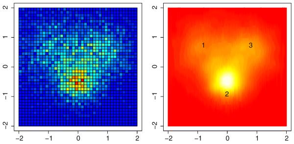
An example of how the neural model explains the raw data (left panel) through a finite mixture of normal distributions (right panel). Voxels that have larger degrees of activity are translated to regions of larger activation in the corresponding source of the normal mixture model.

The joint model

To generate the data from this experiment, we first obtained parameter values for the cognitive model θ and the neural model δ by sampling from known values of the hyperparameters ϕ and Σ. To generate the parameter values, we assumed a direct connection between the level of discriminability d and the degree of relative activation of the first brain source π₁. To enforce this relationship, we generated a value for the parameter d and the parameter π₁ for each subject by sampling from a bivariate normal distribution. We enforced a strong positive relationship between these two variables such that ρ=0.7. The rationale is that the first source might correspond to memory retrieval ability, and that as the degree of relative source activation increases, the ability of the subject to remember whether or not an item was on the previously studied list will increase, resulting in higher discriminability or d in the SDT model.

Once all of the parameter values had been generated for the behavioral (i.e., θ={d,b}) and the neural (i.e., δ={π,μ,ξ}) models, we used each parameter set to generate a corresponding data set, as described above. We generated data for 100 subjects experiencing 100 trials.

Results

To fit the joint model to the (simulated) data, we used a blocked version of differential evolution with Markov chain Monte Carlo (DE-MCMC; see ter Braak, 2006; Turner et al., in press) and made standard choices for the tuning parameters.¹ Standard assessments of convergence were applied, and we found that each of the parameter values was suitably recovered. Because the data were simulated, we were able to initialize the chains to values with high posterior density. We ran the algorithm with 36 chains operating in parallel for 2000 iterations, and treated the first 1000 iterations as a burn in period. Thus, we obtained 36,000 samples from the joint posterior distribution.

Once the joint model had been fit to the data, we were able to use the parameter estimates to examine the relationships between the behavioral and neural data. For example, we found that the estimate for the correlation between discriminability and the degree of activation at Source 1 was approximately r=.65, reflecting a strong positive relationship between these two model parameters. Had the model been fit to real data, we could then apply interpretations to this estimate and make substantive conclusions about how the particular location in the brain (i.e., Source 1) was related to recognition ability.

We can also use the joint model to highlight an advantage of our approach. Specifically, given only partial information about a particular subject, we can make predictions from the model about the missing data. For example, suppose we were able to obtain behavioral data for a particular subject, but were unable to obtain fMRI data. Fitting the joint model to the data would allow us to generate a predictive distribution for the pattern of source activation based on the relationships between the behavioral and neural models inferred from the group data. We can then take the predicted pattern of source activation from the neural model to produce a predicted pattern of activation at the voxel level. This process can even be reversed so that if we were able to obtain only neural data for a particular subject, we could make predictions about what the hit and false alarm rates could have been, conditional on the pattern of brain activity observed in the fMRI scan.

To illustrate this feature of the model, we also fit the joint model to the data of four subjects having only partial observations. Specifically, two of the subjects were simulated so that only neural data were obtained in the form of a fMRI scan and the other two subjects were simulated to have only behavioral data (i.e., the number of hit and false alarms). The goal was then to make predictions for the data that were not obtained for each of these subjects.

Predicting behavioral data from neural data

For the first two partially observed subjects, we obtained only neural data. The neural data were assumed to have been gathered in the same way as all of the other subjects (as described above). The model was fit to the full data set including the partially observed subjects and we used this information to obtain predictions about the distribution of behavioral data that we would have obtained, had we collected the behavioral data.

Because we use a Bayesian approach to fitting our joint model to the data, we can easily make predictions about unobserved data. The model first obtains information from the neural data by estimating the parameters of the neural model. Then, the model sends the information contained in the parameter estimates up to the hyperparameters ϕ and Σ. The hyperparameters have information about the structural relationships between the neural model parameters and the cognitive model parameters, and this information is driven by the subjects who were fully observed. Using the information contained in ϕ and Σ, we can then make predictions about the parameter estimates for the cognitive model, in this case the SDT model parameters θ={d,b}. Finally, using the parameter estimates for the cognitive model, we can make predictions about the hit and false alarm rates that would have been obtained, given the neural data.

Fig. 4 shows an example of how this process works for two subjects, one subject having a small Source 1 activation (top row) and the second having a larger Source 1 activation (bottom row). The left panels show the neural data for these two subjects at the voxel level. Estimates for the neural model parameter δ are obtained from these data and then passed upward to the joint model's hyperparameters ϕ and Σ. The middle panels show a representation (i.e., the posterior predictive distribution) of the relationship between the activation of Source 1 (the x-axis) and the level of discriminability (the y-axis). The relationship between these model parameters is inferred from the full data, driven by the subjects for whom both neural and behavioral data have been obtained. The dashed vertical red lines show the level of Source 1 activation for each subject (π₁=0.3 in the top middle panel and π₁=0.46 in the bottom panel). Using the hyperparameters, the model then makes a prediction for what the parameter estimates for discriminability would have been (not shown) and converts this prediction into a distribution over hit and false alarm rates. The predicted behavioral data are shown as the gray clouds in the right panels of Fig. 4. As a guide, reference lines corresponding to d=0 (the diagonal line), d=1 (the middle curved line), and d=2 (the line with the sharpest curve) are shown and the means of the predicted hit and false alarm rates are shown as the black “x” symbols. The figure shows that for the subject with a smaller Source 1 activation, the model predicts that that subject will tend to have lower discriminability than the subject with a larger Source 1 activation.

Fig. 4.

Two examples of predictions made from the joint model given only neural data. The rows correspond to the two different subjects — the first row represents a subject with low Source 1 activation and the bottom row represents a subject with high Source 1 activation. The left panels show two simulated subjects having only neural data (i.e., no behavioral data). The middle panel plots the joint distribution of the activation of Source 1 against discriminability, a relationship that was inferred from the full set of data. The red vertical dashed lines represent the estimated degree of Source 1 activation in the corresponding row (see the left panel). The right panels show the predicted distribution of hit (y-axis) and false alarm (x-axis) rates made by the model along with the mean prediction (shown as the black “x” symbol), conditional on the neural data in the corresponding row. Reference lines of d={0,1,2} are also show in the right panels.

Predicting neural data from behavioral data

We also examined the model predictions for neural data, given only behavioral data. The ability of the joint model to make these predictions is important from a cost and ethical point of view, because neural data can often be expensive and time consuming to obtain (e.g., fMRI). The ability to predict neural activity from behavioral data alone could be particularly useful in the clinical setting, where the exact structure of affected brain regions in unhealthy subjects can be difficult to pinpoint. Furthermore, the joint modeling framework could be used on preliminary data to aid in designing new experiments that better identify these affected regions or better test psychological theory (Myung and Pitt, 2009).

To examine the model predictions, we fit the joint model to the full data set, but included two subjects for whom only behavioral data were obtained. As in the above example, the model can easily make predictions for neural data given only the behavioral data after uncovering the relationships between the neural and cognitive model parameters. When only behavioral data have been observed, the information is passed in the opposite direction as described in the previous example.

Fig. 5 shows an example of this process for two subjects, one of which had low discriminability (top row; d=0.8) and one of which had high discriminability (bottom row; d=1.5). The left panels show the obtained hit and false alarm rates, along with reference lines for different levels of discriminability. From these data, the model obtains estimates for the cognitive model parameters θ, which are then passed upward to the hyperparameters. The middle panels again show a representation of the relationship between the Source 1 activation and the level of discriminability, which is inferred from the group of subjects for whom both neural and behavioral data were obtained. The red horizontal dashed lines show an estimate of the level of discriminability inferred from the behavioral data. The estimate for discriminability is then used in combination with the hyperparameters to make predictions for the neural model parameters (not shown), which are then used to make predictions for the pattern of activity that might have been observed at the voxel level. These patterns of activity are shown in the right panels of Fig. 5. The model shows that as the hit rate increases and the false alarm rate decreases (resulting in greater accuracy), the degree of Source 1 activation becomes stronger. In addition, because the degree of activation parameters π are constrained to sum to one and the degree of activation of Source 2 was held constant, the activation of Source 3 decreases to account for the increase in Source 1 activation.

Fig. 5.

Two examples of predictions made from the joint model given only behavioral data. The rows correspond to the two different subjects — the first row represents a subject with low discriminability and the bottom row represents a subject with high discriminability. The left panels show two simulated subjects having only behavioral data (i.e., no neural data) in the form of a hit (y-axis) and false alarm (x-axis) rate, shown as the “x” symbol. Reference lines of d={0,1,2} are shown in the left panels. The middle panels show the joint distribution of the activation of Source 1 against discriminability, a relationship that was inferred from the full set of data. The red horizontal dashed lines represent the estimated discriminability (i.e., the parameter d) from the data in the corresponding row (see the left panels). The right panels show the predicted distribution of neural data at the voxel level.

This section has illustrated a few of the benefits of our joint modeling approach. Namely, one can combine behavioral and neural models together to form one unified model to account for both sources of data. Using such a framework, we can infer the relationships among the model parameters in a principled and automatic way. Finally, as a direct result of our Bayesian approach, we can easily make predictions about data that were not observed.

Fitting the joint model to response time and tract strength data

In this section, we will demonstrate the joint model's ability to generalize and predict future data for new subjects while having only neural data or some combination of neural data and (sparse) behavioral data. We demonstrate this feature of the model on experimental data reported in Forstmann et al. (2011). The study was designed to provide further evidence for the striatal hypothesis of the speed accuracy tradeoff (Bogacz et al., 2010; Forstmann et al., 2008, 2010), which asserts that under time pressure, the striatum decreases the activation of the output nuclei of the basal ganglia, thereby releasing the brain from inhibition and facilitating decisions that are fast but error-prone (Mink, 1996; Smith et al., 1998). The data were collected to further investigate whether age-related slowing might be related to the degeneration of corticostriatal connections, often measured by structural diffusion-weighted imaging (DWI).

Experiment

The data were presented in Forstmann et al. (2011) and were produced by 20 young subjects and 14 elderly subjects. The experiment used a moving dots task where subjects were asked to decide whether a cloud of semi-randomly moving dots appeared to move to the left or to the right. Subjects indicated their response by pressing one of two spatially compatible buttons with either their left or right index finger. Before each decision trial, subjects were instructed whether to respond quickly (the speed condition), accurately (the accuracy condition), or at their own pace (the neutral condition). Following the trial, subjects were provided feedback about their performance. In the speed and neutral conditions, subjects were told that their responses were too slow whenever they exceeded a RT of 400 and 750 ms, respectively, for the young subjects and 470 and 820 ms for the elderly subjects, respectively. In the accuracy condition, subjects were told when their responses were incorrect. Each subject completed 840 trials, equally distributed over the three conditions.

The cognitive model

To model the behavioral data, we chose the mathematically simple LBA model (Brown and Heathcote, 2008), consistent with Forstmann et al. (2008, 2010, 2011). The LBA model reduces the evidence accumulation process assumed by previous models of choice RT, such as competition between alternatives (e.g., Brown and Heathcote, 2005; Usher and McClelland, 2001), passive decay of evidence (“leakage”, e.g., Usher and McClelland, 2001), and even within trial variability (e.g., Ratcliff, 1978; Stone, 1960). The model's simplicity allows closed-form expressions for the first passage time distributions for each accumulator. With these equations, one can specify the likelihood function for the model parameters, which has been instrumental in the LBA model's success (e.g., Donkin et al., 2009a, 2009c, 2011; Forstmann et al., 2008, 2010, 2011; Ludwig et al., 2009).

Fig. 6 shows a graphical representation of the LBA model for two-choice data. Each response option c={1,…,C} is represented as a single accumulator (i.e., the left and right panels). Following the presentation of a stimulus, evidence ballistically accumulates for each alternative until one of the alternatives reaches the threshold b. The model assumes some initial amount of evidence is present for each response option. Specifically, each accumulator begins with an independent amount of starting evidence k_c, which is sampled independently for each accumulator from a (continuous) uniform distribution so that k_c~CU[0,A]. The rate of evidence accumulation for the cth option d_c is sampled independently for each accumulator from a normal distribution with mean v_c and standard deviation s. As a result, the rate of evidence will vary between trials, but will have the same expected value. Finally, the LBA model assumes that the observed RT is the sum of the decision time, plus some extra time τ for the nondecision process such as motor execution (a parameter that is not shown in Fig. 6). For simplicity, τ is usually assumed to be constant across trials. Thus, the final observed RT is given by

$$\mathit{RT}=\underset{c}{\mathit{min}}\left(\frac{b-k_c}{d_c}\right)+\tau .$$

Fig. 6.

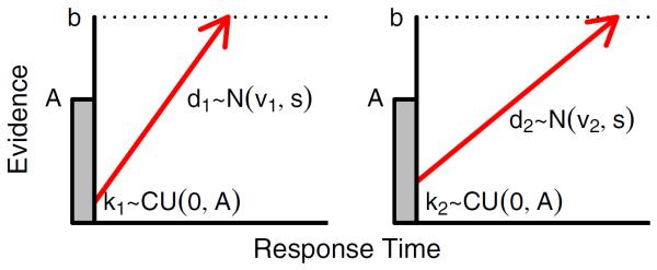
The linear ballistic accumulator (LBA) model. The LBA model represents response alternatives by two accumulators (i.e., the left and right panels). Upon the presentation of a stimulus, the two accumulators gather evidence ballistically and race to reach the threshold b. The observer then selects the response alternative that corresponds to the accumulator that reaches the threshold first. Both the rate of evidence accumulation and the initial amount of evidence vary from trial to trial.

To satisfy scaling conditions of the model, it is common to set the standard deviation of the sampled drift rates to one, so s=1, but other constraints are possible (see Donkin et al., 2009b).

We denote the response time for the jth subject on the ith trial as RT_j,i and the response choice as RE_j,i. To simultaneously explain both RT and choice, we require the “defective” distribution for the ith accumulator, which is the probability of the cth accumulator reaching the threshold and the other accumulators not reaching the threshold. The density function for this distribution is given by

$$\text{LBA}(c,t\mid b,A,v,s,\tau )=f(c,t)\prod _{k\ne c}(1-F(k,t\left)\right),$$ (2)

where v={v₁,…,v_C}, f(c,t) and F(c,t) are the PDF and cumulative density function (CDF) for the time taken for the cth accumulator to reach the threshold, respectively (see Brown and Heathcote, 2008; Turner et al., in press, for details). To incorporate the nondecision time parameter into the PDF, we substitute (t–τ) for t in Eq. (2). Thus, the behavioral data for the jth subject B_j={RE_j,RT_j}, and we write the likelihood function for the jth subject as

$$L\left({\theta }_j\mid B_j\right)=\prod _{i=1}^N\text{LBA}\left({\mathit{RE}}_{j,i},{\mathit{RT}}_{j,i}\mid b_j,A_j,v_j,s,{\tau }_j\right),$$

where θ_j={b_j,A_j,v_j,s,τ_j}.

Because there are three speed conditions in the experiment, we use a vector of response threshold parameters $b_j=\{b_j^{\left(1\right)},b_j^{\left(2\right)},b_j^{\left(3\right)}\}$ so that $b_j^{\left(1\right)}$, $b_j^{\left(2\right)}$ and $b_j^{\left(3\right)}$ are used for the accuracy, neutral and speed conditions of the experiment for the jth subject, respectively. We constrained the upper bound of the start point A to be equal across the emphasis conditions.

Neural model

DWI relies on the Brownian motion of water molecules. It is possible to fit a tensor model to the data and subsequently compute probabilistic tractography (Behrens et al., 2003). This allows one to estimate tract strength, a probabilistic white matter connectivity measure, between different cortico-subcortical brain regions. Based on previous results, four different tract strength measures – between the left and right pre-SMA into the left and right striatum – were taken (see Fig. 7 and Forstmann et al., 2008).

Fig. 7.

Tract strength was computed between cortico (pre-SMA) and subcortical (striatum) brain areas (Forstmann et al., 2011).

We use N_j,m to denote the mth tract strength measurement for the jth subject and use a single parameter δ_j to model the mean tract strength measurement such that

$$\mathrm{logit}\left(N_{j,m}\right)~\mathcal{N}\left({\delta }_j,1.0\right).$$

We set the standard deviation of the normal distribution over the logit of the tract strengths to equal one because we were not interested in relating the variance in the tract strength measurements to the cognitive model parameters and because it reflected the empirical standard deviation of tract strengths from the experiment. We used the logit transformation on the tract strength measurements out of convenience so that the normal distribution, which has infinite support, could be used to model these measurements.

Joint model

To combine both the behavioral and the neural models into a single, unified model, we begin by specifying the hyperparameter vector

$$\varphi =\left[{\delta }_{\mu },b_{\mu }^{\left(1\right)},b_{\mu }^{\left(2\right)},b_{\mu }^{\left(3\right)},A_{\mu },v_{\mu }^{\left(1\right)},v_{\mu }^{\left(2\right)},{\tau }_{\mu }\right],$$

which contains the mean parameters for each of the subject-level parameters. We then combine all of the hyper variances of the subject-level parameters together to form the matrix Σ, so that

where

$${\theta }_{\sigma }^2=\left[\begin{array}{ccccccc}\hfill {\left(b_{\sigma }^{\left(1\right)}\right)}^2\hfill & \hfill 0\hfill & \hfill 0\hfill & \hfill 0\hfill & \hfill 0\hfill & \hfill 0\hfill & \hfill 0\hfill \\ \hfill 0\hfill & \hfill {\left(b_{\sigma }^{\left(2\right)}\right)}^2\hfill & \hfill 0\hfill & \hfill 0\hfill & \hfill 0\hfill & \hfill 0\hfill & \hfill 0\hfill \\ \hfill 0\hfill & \hfill 0\hfill & \hfill {\left(b_{\sigma }^{\left(3\right)}\right)}^2\hfill & \hfill 0\hfill & \hfill 0\hfill & \hfill 0\hfill & \hfill 0\hfill \\ \hfill 0\hfill & \hfill 0\hfill & \hfill 0\hfill & \hfill A_{\sigma }^2\hfill & \hfill 0\hfill & \hfill 0\hfill & \hfill 0\hfill \\ \hfill 0\hfill & \hfill 0\hfill & \hfill 0\hfill & \hfill 0\hfill & \hfill {\left(v_{\sigma }^{\left(1\right)}\right)}^2\hfill & \hfill 0\hfill & \hfill 0\hfill \\ \hfill 0\hfill & \hfill 0\hfill & \hfill 0\hfill & \hfill 0\hfill & \hfill 0\hfill & \hfill {\left(v_{\sigma }^{\left(2\right)}\right)}^2\hfill & \hfill 0\hfill \\ \hfill 0\hfill & \hfill 0\hfill & \hfill 0\hfill & \hfill 0\hfill & \hfill 0\hfill & \hfill 0\hfill & \hfill {\tau }_{\sigma }^2\hfill \end{array}\right],$$

and

$$\rho {\delta }_{\sigma }{\theta }_{\sigma }=\left[b_{\sigma }^{\left(1\right)}{\delta }_{\sigma }{\rho }_1{b}_{\sigma }^{\left(2\right)}{\delta }_{\sigma }{\rho }_2{b}_{\sigma }^{\left(3\right)}{\delta }_{\sigma }{\rho }_3{A}_{\sigma }{\delta }_{\sigma }{\rho }_4{v}_{\sigma }^{\left(1\right)}{\delta }_{\sigma }{\rho }_5{v}_{\sigma }^{\left(2\right)}{\delta }_{\sigma }{\rho }_6{\tau }_{\sigma }{\delta }_{\sigma }{\rho }_7\right].$$

Here we can see that Σ is partitioned to reflect that other matrices fill the partition with meaningful constraints. For example, the variances for the subject-level parameters are all contained in the matrix ${\theta }_{\sigma }^2$, which is a diagonal matrix. Thus, we do not model the relationships between the cognitive model parameters, although we can still explore them by examining their joint posterior distribution once the model has been fit to the data. What is crucial for the joint model, however, is that the relationships between the cognitive model and the neural model are inferred by means of the matrix (i.e., a vector in this example) ρδ_σθ_σ. These relationships will be directly modeled through the correlation parameter vector ρ. Finally, for the parameters δ_j and θ_j for each Subject j, we assume the common structure

$$\left({\delta }_j,{\theta }_j\right)~{\mathcal{N}}_8(\varphi ,\Sigma ).$$

Thus, the likelihood function for the parameters δ and θ is given by

$$\begin{array}{cc}\hfill L(\delta ,\theta \mid \varphi ,\Sigma ,B,N)=& \prod _{j=1}^J\left[\prod _{m}p\left(N_{j,m}\mid {\delta }_j\right)\prod _{i}p\left(B_{j,i}\mid {\theta }_j\right)\right]\hfill \\ \hfill & \prod _{j=1}^J\left[\prod _m\mathrm{N}\left(\mathrm{logit}\left(N_{j,m}\right)\mid {\delta }_j,1\right)\prod _i\text{LBA}\left({\mathit{RE}}_{j,i},{\mathit{RT}}_{j,i}\mid b_j,A_j,v_j,s,{\tau }_j\right)\right],\hfill \end{array}$$

where N(x|a,b) denotes the normal density with mean parameter a and standard deviation b at the location x.

In the Bayesian framework, we must also specify prior distributions for each of the group-level parameters. We specified mildly informative priors for each of the hyper mean parameters, so that

$${\delta }_{\mu }~\mathcal{N}(0,10),$$

$$b_{\mu }^{\left(k\right)}~\mathcal{TN}(1,2,0,\infty ),$$

$$A_{\mu }~\mathcal{TN}(1,2,0,\infty ),$$

$$v_{\mu }^{\left(c\right)}~\mathcal{TN}(2,4,0,\infty ),\text{and}$$

$${\tau }_{\mu }~\mathcal{TN}(0.5,1,0,\infty ),$$

where k={1,2} and $\mathcal{TN}(a,b,c,d)$ denotes the underlying truncated normal distribution with mean parameter a, standard deviation b, lower bound c and upper bound d, and mildly informative priors for the hyper standard deviation parameters, so that

$${\delta }_{\sigma }~\Gamma (1,1),$$

$$b_{\sigma }^{\left(k\right)}~\Gamma (1,1),$$

$$A_{\sigma }~\Gamma (1,1),$$

$$v_{\sigma }^{\left(c\right)}~\Gamma (1,1),\text{and}$$

$${\tau }_{\sigma }~\Gamma (1,1).$$

Because we wanted to avoid any speculation about the relationships between the behavioral and neural model parameters, we specified noninformative priors for each of the correlation parameters, such that

$$\rho ~\mathit{CU}(-1,1).$$

Specifying the model in this way allows for easy computation of the Bayes factor via the Savage–Dickey density ratio (see Dickey, 1971; Dickey and Lientz, 1970; Friston and Penny, 2011; Wetzels et al., 2010).

Given the priors listed above, the full joint posterior distribution for the model parameters is given by

$$\begin{array}{cc}\hfill p(\delta ,\theta ,\varphi ,\Sigma \mid B,N)& \propto L(\delta ,\theta \mid \varphi ,\Sigma ,B,N)\prod _{j=1}^{J}p\left({\left[{\delta }_j,{\theta }_j\right]}^{⊺}\mid \varphi ,\Sigma \right)p\left(\varphi \right)p\left(\Sigma \right)\hfill \\ \hfill & \propto L(\delta ,\theta \mid \varphi ,\Sigma ,B,N)\prod _{j=1}^{J}p\left({\left[{\delta }_j,{\theta }_j\right]}^{⊺}\mid \varphi ,\Sigma \right)p\left({\theta }_{\mu }\right)p\left({\delta }_{\mu }\right)p\left({\theta }_{\sigma }\right)p\left({\delta }_{\sigma }\right)p\left(\rho \right),\hfill \end{array}$$

where ${\theta }_{\mu }=\{b_{\mu }^{\left(1\right)},b_{\mu }^{\left(2\right)},b_{\mu }^{\left(3\right)},A_{\mu },v_{\mu }^{\left(1\right)},v_{\mu }^{\left(2\right)},{\tau }_{\mu }\}$.

Results

To fit the joint model to the data, we again used a blocked version of DE-MCMC with the same choices as above for the tuning parameters. We used the DE local-to-best method to obtain starting points with high posterior density (Turner and Sederberg, 2012). We ran the algorithm with 24 chains operating in parallel for 5000 iterations, and treated the first 1000 iterations as a burn in period. Thus, we obtained 96,000 samples from the joint posterior distribution.

There are a number of ways to assess the fit of the model to the data, but for brevity, we report only a few of these ways here. Fig. 8 shows the estimated posterior distribution for the correlations between the single neural model hyperparameter δ and the cognitive model parameters: threshold parameter for the accuracy condition (b⁽¹⁾; top left panel), threshold parameter for the neutral condition (b⁽²⁾; top middle panel), threshold parameter for the speed condition (b⁽³⁾; top right panel), the upper bound of the start point parameter (A; bottom left panel), the drift rate for correct (v⁽¹⁾; bottom middle panel) and the drift rate for incorrect (v⁽²⁾; bottom right panel) responses. The correlation between the nondecision time parameter τ and δ is not shown (it had no substantial correlation). The relationships between the parameters are weak, but the figure does indicate a moderate inverse relationship between response threshold and tract strength for at least the accuracy and neutral conditions and a moderate positive relationship between the drift rate for the correct responses and tract strength. Taken together, these patterns suggest that as tract strength increases, subjects will tend to require less information to make a decision and will make this decision with greater accuracy.

Fig. 8.

The estimated posterior distributions for six of the seven correlation parameters.

If we wished to perform significance tests, at this point we could evaluate the probability of a particular hypothesis by analyzing the posterior distribution. For example, suppose we wished to test the hypothesis that the rate of evidence accumulation for a correct response was significantly positively related to the level of tract strength. We could then integrate the marginal posterior distribution of the parameter ρ₅, which represents the correlation between $v_{\mu }^{\left(1\right)}$ and δ_μ, to obtain an estimate for the probability of a positive relationship between the two variables. For these data, we found this probability to be 0.836, which provides evidence that there exists a positive correlation between these two variables.

To examine this relationship further, we examined the posterior predictive distributions of the joint model. Fig. 9 shows the posterior predictive distributions (gray clouds) along with the observed data (black dots) for each of the speed emphasis conditions (columns). We examined the relationship between tract strength and RT in two ways. First, we examined how tract strength was related to the mean RT at the individual level, shown in the top row. To generate the posterior predictive density, we generated 1000 tract strength values and choice RT pairs for 1000 parameter sets (θ_j,δ_j), which were sampled from the joint posterior distribution corresponding to each subject j. The mean RT was calculated for each simulated data set, collapsing across the choice variable. The figure shows that there is a slight negative relationship between tract strength and the mean RT.

Fig. 9.

Posterior predictive distributions for the mean RT by tract strength at the individual subject level (top row) and the group level (bottom row) for each speed emphasis condition (columns) from the joint model (gray clouds). The observed data overlay each plot (black dots).

We also examined how the mean RT was related to tract strength at the group level (bottom row). To generate this posterior predictive density, we first sampled a value for ϕ and Σ from their estimated posterior distributions. We then generated hypothetical parameter values for (θ,δ), which were then used to generate values for tract strength and choice RT pairs in the same way as in the top panel. The generated posterior predictive density is important because it is a generalization of the pattern between the neural and behavioral model parameters that is learned by the joint model from the data. The figure illustrates a strong negative relationship between tract strength and mean RT: as tract strength increases, the mean RT tends to decrease. The strength of this relationship decreases across the emphasis conditions such that as speed is further stressed, the correlation between tract strength and mean RT decreases.

While Fig. 9 does show the basic predictions of the model as a function of tract strength, it is not obvious how the predictions of the full RT distribution might vary as a function of tract strength. It is also unclear how the neural data affects the predictions of the joint model when compared with a behavioral model that ignores the neural data. To explore this, we performed a simulation study with two conditions of withheld data. In the first condition, we removed all observations from two of the 24 subjects: one subject had a high average tract strength value (0.973) and one had a low tract strength value (0.405). In the second condition, we removed only 50% of the data from the same two subjects. Both the joint and behavioral models were fit to the data from each condition and the maximum a posterior (MAP) estimates were calculated from the joint posterior distributions. The MAP estimates were then used to generate a posterior predictive density estimate, which we summarized by calculating the median prediction for all choice RT pairs.

Fig. 10 shows the results of the simulation study for the accuracy condition. The left panel shows the raw data for the low tract strength subject (dashed black lines) and the high tract strength subject (solid gray lines). In each panel, the correct RT distributions are shown on right whereas the incorrect RT distributions are shown on the left. The right panel shows the posterior predictive distributions for the joint (top) and behavioral (bottom) models for the first (i.e., the condition where 100% of the behavioral data were withheld) and second conditions (i.e., the condition where only 50% of the behavioral data were withheld), respectively. For the first condition, the figure shows that the predictions for the behavioral model do not differ across the two subjects because the model has no information that can be used to dissociate one subject from another. On the other hand, the predictions from the joint model show a clear separation between the two subjects as a result of the information learned from the neural data of the two subjects and the relationship learned between the behavioral and neural model parameters from the remaining 22 subjects. In particular, the joint model correctly predicts that the high tract strength subject will tend to produce faster and more accurate responses than the low tract strength subject.

Fig. 10.

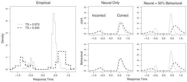
A model prediction comparison for a subject with a high average tract strength measurement (gray solid lines) and a subject with a low average tract strength measurement (dashed black lines). The left panel shows a histogram of the raw data whereas the right panels show the predictions of the joint (top) and the behavioral (bottom) models under two conditions: the left column corresponds to a condition in which all behavioral data are withheld and the right column corresponds to a condition in which only 50% of the behavioral data are withheld. Only the joint model is able to differentiate the predictions for the two subjects when only neural data is available. In each panel, the RT distribution for incorrect responses is shown on the left whereas the RT distribution for correct responses is shown on the right.

While the neural data for this real-world experiment are sparse, the joint model is able to identify a signal in the data that is amplified in the hierarchical model. However, due to the sparsity of the neural data, a principled model would predict that as the number of observations from the behavioral data grows, the predictions of the joint and behavioral models should quickly converge because the proportion of shared information between the two models increases. The right panel of Fig. 10 shows that this is indeed the case: the predictions of the joint and behavioral models are nearly identical when 50% of the behavioral data are available. Furthermore, the predictions of both models accurately reflect the patterns of observed data from the two withheld subjects (leftmost panel).

General discussion

We have presented a new approach to unifying neural and cognitive models to better understand cognition. In contrast to previous methods, our method is extremely flexible because it can combine any neural model with any cognitive model. Our method also provides a way to infer the relationships that might exist between the biological and physical properties of the brain and higher-level cognitive processes.

By combining two separate models into a single Bayesian hierarchical model, we can make predictions about missing data. In our simulation study, we showed that when only neural data are available, the model can use the structural relationships between the model parameters inferred from the group to make predictions about behavioral data. The same feature of the model can also be used to make predictions about the relationships between behavioral and neural model parameters at the group level. For example, the joint posterior distributions for cognitive parameters and fMRI activation shown in Figs. 4 and 5 show what the model predicts the relationship will be between these two variables in general. The model develops these predictions based solely on the data that were observed.

We have also demonstrated that the joint model can predict future behavioral data from new subjects based only on the neural data associated with those subjects. The joint model accomplishes this by learning the structural relationships between the neural and behavioral model parameters from the group of available subjects, and then generalizes this information to new subjects. By contrast, behavioral models that learn only from behavioral data cannot differentiate between subjects because they do not use the neural data. Generally, any joint model will need to explicitly establish a link between neural and behavioral data to accomplish this generalization or prediction task.

While we did not fully exploit the importance of constraining the neural model parameters in the examples presented in this article, we speculate that constraining these parameters can help identify important neural signatures, which are often masked by the noise inherent in neural data. The added constraint could prove useful in developing richer, theoretically motivated models of neural data.

By using flexible hyperparameter structures we can also infer which relationships between the model parameters are important. That is, we are not limited to investigating only a priori hypotheses, as in the model-based imaging approach (O'Doherty et al., 2007). This makes our approach suited to exploratory studies once proper adjustments have been made to the prior odds term (Stephens and Balding, 2009). To infer those relationships, we need only specify a correlation structure between the parameters of interest. The magnitude of the relationship manifests in the marginal posterior distribution of the correlation parameter. Using the estimate of the correlation parameter, we can then assess the importance of the relationship by examining summary statistics or regions of interest of the posterior (e.g., a region of practical equivalence analysis; see Kruschke, 2011).

Another important feature of our framework is that it is not limited to a particular pair of models or type of data. That is, any cognitive model of interest can be combined with any neural model of interest within the joint modeling framework, as long as likelihood functions are available for both. Similarly, we are not restricted to particular types of data. We choose a neural/behavioral model to explain the neural/behavioral data, and in this way, we have unlimited flexibility in modeling the joint distribution of the data.

Finally, our modeling approach applies constraints to the model parameters in a principled way. Other approaches rely on only the behavioral data to inform the estimation procedure. As a result, these approaches are unable to use the neural data to inform the parameter estimates for behavioral models. By contrast, our approach uses these properties to restrain parameter estimates to conform to more biologically-plausible scenarios. In this way, our approach provides a unifying account of both applied and theoretical explanations of cognition. Providing such a framework enables more informative predictions for future (i.e., unobserved) data on the basis of the data that were observed.

Limitations

Despite the potential of our approach, there are several limitations. First, using the correlation parameter of a multivariate normal distribution may not be the best choice to understand the relationships between model parameters. For example, if one were interested in causal relationships between neural sources and cognitive mechanisms, a discriminative approach such as structural equation modeling or generalized linear modeling would be more useful. However, such a model specification would still fit within the proposed framework. To do so, one would specify that say, the cognitive model parameters, are a function of the neural sources. For example, one could specify a linear relationship between the neural and cognitive model parameters, so that

$$\theta =\delta \beta +∊,$$

where β is the standard coefficient matrix for linear regression and ε specifies the error term. Here, we have defined a structural relationship between two latent parameters; however, one could image a scenario where the parameters δ were the neural data themselves. For example, in the data from the experiment above, one could specify that

$$\delta =\frac{1}{M}\sum _{m=1}^M{N}_{j,m}.$$

Here, δ becomes a deterministic node in the model and can be used to enforce a stronger constraint on the cognitive model parameters θ. In some preliminary studies, we have examined functional approaches like the one described here. However, causal relationships are meant more for confirmatory purposes (e.g., to confirm a hypothesis) whereas the approach we present in this article is meant for exploratory purposes. We believe that the latter is more applicable to the generative study of cognition.

Another limitation comes directly from the model structure. Specifically, the constraint from the group-level model parameters could be conceived of as a limitation of our model. In some preliminary studies, we have found that specifying priors for subject-level parameters may be overly restrictive in some cases, such as when there are few observations at the subject-level. In this situation, because little is known at the subject level, the model will resort to using the information contained in the prior and the estimates for the subject-level parameters may systematically differ from estimates that would have been obtained without the specification of a prior, an effect known as shrinkage.

However, the way that Bayesian models handle sparse data can also be seen as a benefit of our approach. When little is known about individual subjects, hierarchical Bayesian models learn a little from each subject and this information is passed back and forth between the group- and subject-level parameters. This same information sharing scheme is what facilitates the prediction of one source of data, e.g., the neural data, having only observed the behavioral data. To remedy the problem of overly harsh prior specification, one can use more flexible distributions to characterize the distribution of subject-specific model parameters. For example, one could use nonparametric Bayesian techniques (Gershman and Blei, 2012; Navarro et al., 2006), which allow the model to learn the most appropriate representation of the distribution of subject-specific parameters. Such a flexible representation would help to attenuate the problem of parameter shrinkage.

Throughout the manuscript, we focused on linking behavioral and neural model parameters together across subjects (see Eq. (1)). However, the joint modeling framework can be further extended to the individual subject level, where parameters for each trial can be linked together. To do this, we need only specify that the individual trial parameters are correlated for each individual subject. We could then specify a structure for the subject-specific correlation parameters in a three-level hierarchy. Such an extension is particularly useful for neural data, which are often obtained on a trial-to-trial basis.

A final limitation is in our specification of the covariance matrix Σ. For the models in this article, we set the off-diagonal elements to zero because the correlations among the behavioral and neural model parameters were not theoretically important. While this particular constraint is useful in minimizing the computational complexity associated with estimating the parameters of the hierarchical model, such a constraint could have negative implications. For example, if the model were misspecified such that a strong (i.e., having a large magnitude) correlation existed between the model parameters, the misspecification would manifest as a bias in the estimates of the remaining parameters. In practice, we recommend investigating a variety of model constraints so that simplifying assumptions can be properly justified.

Conclusions

In this article, we have presented a hierarchical Bayesian framework for combining both neural and cognitive models into a single unifying model. We have shown that our approach provides a number of benefits over current approaches and allows for principled inference of the relationships between the biological properties of the brain assessed by neuroimaging techniques and the theories of cognition that are used to understand higher levels of cognitive processing. With this approach, one can investigate neural and behavioral data using any combination of neural and cognitive models. By unifying the two seemingly different aspects of cognitive processing, we have presented a step toward a better understanding of cognition.

References

- Anderson JR. How Can the Human Mind Occur in the Physical Universe? Oxford University Press; New York, NY: 2007. [Google Scholar]
- Anderson JR, Qin Y, Jung KJ, Carter CS. Information-processing modules and their relative modality specificity. Cogn. Psychol. 2007;54:185–217. doi: 10.1016/j.cogpsych.2006.06.003. [DOI] [PubMed] [Google Scholar]
- Anderson JR, Carter CS, Fincham JM, Qin Y, Rosenberg-Lee M, S. M. R. Using fMRI to test models of complex cognition. Cogn. Sci. 2008;32:1323–1348. doi: 10.1080/03640210802451588. [DOI] [PubMed] [Google Scholar]
- Anderson JR, Betts S, Ferris JL, Fincham JM. Neural imaging to track mental states. Proc. Natl. Acad. Sci. U. S. A. 2010;107:7018–7023. doi: 10.1073/pnas.1000942107. [DOI] [PMC free article] [PubMed] [Google Scholar]
- Anderson JR, Fincham JM, Schneider DW, Yang J. Using brain imaging to track problem solving in a complex state space. NeuroImage. 2012;60:633–643. doi: 10.1016/j.neuroimage.2011.12.025. [DOI] [PMC free article] [PubMed] [Google Scholar]
- Behrens T, Johansen-Berg H, Woolrich MW, Smith SM, Wheeler-Kingshott CA, Boulby PA, Barker GJ, Sillery EL, Sheehan K, Ciccarelli O, Thompson AJ, Brady JM, Matthews PM. Non-invasive mapping f connections between human thalamus and cortex using diffusion imaging. Nat. Neurosci. 2003;6:750–757. doi: 10.1038/nn1075. [DOI] [PubMed] [Google Scholar]
- Bogacz R, Wagenmakers EJ, Forstmann BU, Nieuwenhuis S. The neural basis of the speed–accuracy tradeoff. Trends Neurosci. 2010;33:10–16. doi: 10.1016/j.tins.2009.09.002. [DOI] [PubMed] [Google Scholar]
- Borst J, Anderson JR. Towards pinpointing the neural correlates of ACT-R: a conjunction of two model-based fMRI analyses. In: Rubwinkel N, Drewitz U, van Rijn H, editors. Proceedings of the 11th International Conference on Cognitive Modeling; Berlin. 2012. [Google Scholar]
- Borst JP, Taatgen NA, Hedderik VR. Using a symbolic process model as input for model-based fMRI analysis: locating the neural correlates of problem state replacement. NeuroImage. 2011;58:137–147. doi: 10.1016/j.neuroimage.2011.05.084. [DOI] [PubMed] [Google Scholar]
- Brown S, Heathcote A. A ballistic model of choice response time. Psychol. Rev. 2005;112:117–128. doi: 10.1037/0033-295X.112.1.117. [DOI] [PubMed] [Google Scholar]
- Brown S, Heathcote A. The simplest complete model of choice reaction time: linear ballistic accumulation. Cogn. Psychol. 2008;57:153–178. doi: 10.1016/j.cogpsych.2007.12.002. [DOI] [PubMed] [Google Scholar]
- Dickey JM. The weighted likelihood ratio, linear hypotheses on normal location parameters. Ann. Math. Stat. 1971;42:204–223. [Google Scholar]
- Dickey JM, Lientz BP. The weighted likelihood ratio, sharp hypotheses about chances, the order of a Markov chain. Ann. Math. Stat. 1970;41:214–226. [Google Scholar]
- Dolan RJ. Neuroimaging of cognition: past, present and future. Neuron. 2008;60:496–502. doi: 10.1016/j.neuron.2008.10.038. [DOI] [PMC free article] [PubMed] [Google Scholar]
- Donkin C, Averell L, Brown S, Heathcote A. Getting more from accuracy and response time data: methods for fitting the linear ballistic accumulator. Behav. Res. Methods. 2009a;41:1095–1110. doi: 10.3758/BRM.41.4.1095. [DOI] [PubMed] [Google Scholar]
- Donkin C, Brown S, Heathcote A. The overconstraint of response time models: rethinking the scaling problem. Psychon. Bull. Rev. 2009b;16:1129–1135. doi: 10.3758/PBR.16.6.1129. [DOI] [PubMed] [Google Scholar]
- Donkin C, Heathcote A, Brown S. Is the linear ballistic accumulator model really the simplest model of choice response times: a Bayesian model complexity analysis. In: Howes A, Peebles D, Cooper R, editors. 9th International Conference on Cognitive Modeling — ICCM2009; Manchester, UK. 2009c. [Google Scholar]
- Donkin C, Brown S, Heathcote A. Drawing conclusions from choice response time models: a tutorial. J. Math. Psychol. 2011;55:140–151. [Google Scholar]
- Egan JP. Tech. Rep. AFCRC-TN-58-51. Hearing and Communication Laboratory, Indiana University; Bloomington, Indiana: 1958. Recognition memory and the operating characteristic. [Google Scholar]
- Fincham JM, Anderson JR, Betts SA, Ferris JL. Using neural imaging and cognitive modeling to infer mental states while using and intelligent tutoring system. Proceedings of the Third International Conference on Educational Data Mining (EDM2010); Pittsburgh, PA. 2010. [Google Scholar]
- Flandin G, Penny WD. Bayesian fMRI data analysis with sparse spatial basis functions. NeuroImage. 2007;34:1108–1125. doi: 10.1016/j.neuroimage.2006.10.005. [DOI] [PubMed] [Google Scholar]
- Forstmann BU, Dutilh G, Brown S, Neumann J, von Cramon DY, Ridderinkhof KR, Wagenmakers E-J. Striatum and pre-SMA facilitate decision-making under time pressure. Proc. Natl. Acad. Sci. 2008;105:17538–17542. doi: 10.1073/pnas.0805903105. [DOI] [PMC free article] [PubMed] [Google Scholar]
- Forstmann BU, Anwander A, Schäfer A, Neumann J, Brown S, Wagenmakers E-J, Bogacz R, Turner R. Cortico-striatal connections predict control over speed and accuracy in perceptual decision making. Proc. Natl. Acad. Sci. 2010;107:15916–15920. doi: 10.1073/pnas.1004932107. [DOI] [PMC free article] [PubMed] [Google Scholar]
- Forstmann BU, Tittgemeyer M, Wagenmakers E-J, Derrfuss J, Imperati D, Brown S. The speed-accuracy tradeoff in the elderly brain: a structural model-based approach. J. Neurosci. 2011;31:17242–17249. doi: 10.1523/JNEUROSCI.0309-11.2011. [DOI] [PMC free article] [PubMed] [Google Scholar]
- Frank LR, Buxton RB, Wong EC. Probabilistic analysis of functional magnetic resonance imaging data. Magn. Reson. Med. 1998;39:132–148. doi: 10.1002/mrm.1910390120. [DOI] [PubMed] [Google Scholar]
- Friston K. Bayesian estimation of dynamical systems: an application to fMRI. NeuroImage. 2002;16:513–530. doi: 10.1006/nimg.2001.1044. [DOI] [PubMed] [Google Scholar]
- Friston KJ, Penny W. Post hoc Bayesian model selection. NeuroImage. 2011;56:2089–2099. doi: 10.1016/j.neuroimage.2011.03.062. [DOI] [PMC free article] [PubMed] [Google Scholar]
- Friston K, Penny W, Phillips C, Kiebel S, Hinton G, Ashburner J. Classical and Bayesian inference in neuroimaging. NeuroImage. 2002;16:465–483. doi: 10.1006/nimg.2002.1090. [DOI] [PubMed] [Google Scholar]
- Friston K, Harisson L, Penny W. Dynamic causal modeling. NeuroImage. 2003;19:1273–1302. doi: 10.1016/s1053-8119(03)00202-7. [DOI] [PubMed] [Google Scholar]
- Gershman SJ, Blei DM. A tutorial on Bayesian nonparametric models. J. Math. Psychol. 2012;56:1–12. [Google Scholar]
- Gershman SJ, Blei DM, Pereira F, Norman KA. A topographic latent source model for fMRI data. NeuroImage. 2011;57:89–100. doi: 10.1016/j.neuroimage.2011.04.042. [DOI] [PMC free article] [PubMed] [Google Scholar]
- Gläscher JP, O'Doherty Model-based approaches to neuroimaging: combining reinforcement learning theory with fMRI data. Wires Cognitive Science. 2010;1:501–510. doi: 10.1002/wcs.57. [DOI] [PubMed] [Google Scholar]
- Green DM, Swets JA. Signal Detection Theory and Psychophysics. Wiley Press; New York: 1966. [Google Scholar]
- Guo Y, Bowman FD, Kilts C. Predicting the brain response to treatment using a Bayesian hierarchical model with application to a study of schizophrenia. Hum. Brain Map. 2008;29:1092–1109. doi: 10.1002/hbm.20450. [DOI] [PMC free article] [PubMed] [Google Scholar]
- Hampton AN, Bossaerts P, O'Doherty JP. The role of the ventromedial pre-frontal cortex in abstract state-based inference during decision making in humans. J. Neurosci. 2006:8360–8367. doi: 10.1523/JNEUROSCI.1010-06.2006. [DOI] [PMC free article] [PubMed] [Google Scholar]
- Kershaw J, Ardekani BA, Kanno I. Application of Bayesian inference to fMRI data analysis. IEEE Trans. Med. Imaging. 1999;18:1138–1153. doi: 10.1109/42.819324. [DOI] [PubMed] [Google Scholar]
- Kruschke JK. Doing Bayesian Data Analysis: A Tutorial with R and BUGS. Academic Press; Burlington, MA: 2011. [Google Scholar]
- Lee MD. Special issue on hierarchical Bayesian models. J. Math. Psychol. 2011;55:1–118. [Google Scholar]
- Ludwig CJH, Farrell S, Ellis LA, Gilchrist ID. The mechanism underlying inhibition of saccadic return. Cogn. Psychol. 2009;59:180–202. doi: 10.1016/j.cogpsych.2009.04.002. [DOI] [PMC free article] [PubMed] [Google Scholar]
- Macmillan NA, Creelman CD. Detection Theory: A User's Guide. Lawrence Erlbaum Associates; Mahwah, New Jersey: 2005. [Google Scholar]
- Mazurek ME, Roitman JD, Ditterich J, Shadlen MN. A role for neural integrators in perceptual decision making. Cereb. Cortex. 2003;13:1257–1269. doi: 10.1093/cercor/bhg097. [DOI] [PubMed] [Google Scholar]
- Mink JW. The basal ganglia: focused selection and inhibition of competing motor programs. Prog. Neurobiol. 1996;50:381–425. doi: 10.1016/s0301-0082(96)00042-1. [DOI] [PubMed] [Google Scholar]
- Mumford JA, Turner BO, Ashby FG, Poldrack RA. Deconvolving bold activation in event-related designs for multivoxel pattern classification analyses. NeuroImage. 2012;59:2636–2643. doi: 10.1016/j.neuroimage.2011.08.076. [DOI] [PMC free article] [PubMed] [Google Scholar]
- Myung JI, Pitt MA. Optimal experimental design for model discrimination. Psychol. Rev. 2009;116:499–518. doi: 10.1037/a0016104. [DOI] [PMC free article] [PubMed] [Google Scholar]
- Navarro DJ, Griffiths TL, Steyvers M, Lee MD. Modeling individual differences using Dirichlet processes. J. Math. Psychol. 2006;50:101–122. [Google Scholar]
- Nosofsky RM. Attention, similarity, and the identification–categorization relationship. J. Exp. Psychol. Gen. 1986;115:39–57. doi: 10.1037//0096-3445.115.1.39. [DOI] [PubMed] [Google Scholar]
- O'Doherty JP, Dayan P, Friston K, Critchley H, Dolan RJ. Temporal difference models and reward-related learning in the human brain. Neuron. 2003;28:329–337. doi: 10.1016/s0896-6273(03)00169-7. [DOI] [PubMed] [Google Scholar]
- O'Doherty JP, Hampton A, Kim H. Model-based fMRI and its application to reward learning and decision making. Ann. N. Y. Acad. Sci. 2007;1104:35–53. doi: 10.1196/annals.1390.022. [DOI] [PubMed] [Google Scholar]
- Quirós A, Diez RM, Gamerman D. Bayesian spatiotemporal model of fMRI data. NeuroImage. 2010;49:442–456. doi: 10.1016/j.neuroimage.2009.07.047. [DOI] [PubMed] [Google Scholar]
- Ratcliff R. A theory of memory retrieval. Psychol. Rev. 1978;85:59–108. [Google Scholar]
- Shiffrin RM, Lee MD, Kim W, Wagenmakers E-J. A survey of model evaluation approaches with a tutorial on hierarchical Bayesian methods. Cogn. Sci. 2008;32:1248–1284. doi: 10.1080/03640210802414826. [DOI] [PubMed] [Google Scholar]
- Smith Y, Bevan MD, Shink E, Bolam JP. Microcircuitry of the direct and indirect pathways of the basal ganglia. Neuroscience. 1998;86:353–387. doi: 10.1016/s0306-4522(98)00004-9. [DOI] [PubMed] [Google Scholar]
- Stephens M, Balding DJ. Bayesian statistical methods for genetic association studies. Nat. Rev. Genet. 2009;10:681–690. doi: 10.1038/nrg2615. [DOI] [PubMed] [Google Scholar]
- Stone M. Models for choice reaction time. Psychometrika. 1960;25:251–260. [Google Scholar]
- ter Braak CJF. A Markov chain Monte Carlo version of the genetic algorithm differential evolution: easy Bayesian computing for real parameter spaces. Stat. Comput. 2006;16:239–249. [Google Scholar]
- Turner BM, Sederberg PB. Approximate Bayesian computation with differential evolution. J. Math. Psychol. 2012;56:375–385. [Google Scholar]
- Turner BM, Sederberg PB, Brown S, Steyvers M. Psychological Methods. A method for efficiently sampling from distributions with correlated dimensions. in press. [DOI] [PMC free article] [PubMed] [Google Scholar]
- Usher M, McClelland JL. On the time course of perceptual choice: the leaky competing accumulator model. Psychol. Rev. 2001;108:550–592. doi: 10.1037/0033-295x.108.3.550. [DOI] [PubMed] [Google Scholar]
- Van Gerven MAJ, Cseke B, de Lange FP, Heskes T. Efficient Bayesian multivariate fMRI analysis using a sparsifying spatio-temporal prior. NeuroImage. 2010;50:150–161. doi: 10.1016/j.neuroimage.2009.11.064. [DOI] [PubMed] [Google Scholar]
- Wetzels R, Grasman RPPP, Wagenmakers E-J. An encompassing prior generalization of the Savage–Dickey density ratio. Comput. Stat. Data Anal. 2010;54:2094–2102. [Google Scholar]
- Wilkinson D, Halligan P. The relevance of behavioural measures for functional-imaging studies of cognition. Nat. Rev. Neurosci. 2004;5:67–73. doi: 10.1038/nrn1302. [DOI] [PubMed] [Google Scholar]
- Wu W, Chen Z, Gao S, Brown EN. A hierarchical Bayesian approach for learning sparse spatio-temporal decompositions of multichannel EEG. NeuroImage. 2011;56:1929–1945. doi: 10.1016/j.neuroimage.2011.03.032. [DOI] [PMC free article] [PubMed] [Google Scholar]