Comprehensive Analysis of LC/MS Data Using Pseudocolor Plots

Abstract

We have developed new applications of the pseudocolor plot for the analysis of LC/MS data. These applications include spectral averaging, analysis of variance, differential comparison of spectra, and qualitative filtering by compound class. These applications have been motivated by the need to better understand LC/ MS data generated from analysis of human biofluids. The examples presented use data generated to profile steroid hormones in urine extracts from a Cushing’s disease patient relative to a healthy control, but are general to any discovery-based scanning mass spectrometry technique. In addition to new visualization techniques, we introduce a new metric of variance: the relative maximum difference from the mean. We also introduce the concept of substructure-dependent analysis of steroid hormones using precursor ion scans. These new analytical techniques provide an alternative approach to traditional untargeted metabolomics workflow. We present an approach to discovery using MS that essentially eliminates alignment or preprocessing of spectra. Moreover, we demonstrate the concept that untargeted metabolomics can be achieved using low mass resolution instrumentation.

Introduction

Untargeted analysis of LC/MS data is difficult if not impossible without the use of software designed for this purpose. Numerous software packages have been developed to facilitate these analyses [1–17], and these have all been reviewed recently [18]. Moreover, software provided by manufacturers when an instrument is purchased often enables similar analyses. However, the majority of this type of software requires the user to make a priori decisions concerning which aspects of the data should be considered. While frequently useful, such approaches have a potential for over-processing and filtering and, thus, risk obfuscation of important spectral features. In this work, we demonstrate the value of visualizing all mass spectral intensity data as they relate to one another in chromatographic space with essentially no preprocessing of the data. Spectral profile visualization has been examined in the intensity dimension in other pieces of software [1–5], but to date has apparently been done only for single replicates. Our approach differs in that we evaluate a number of spectra simultaneously. This enables us to examine qualitatively different aspects of spectral profiles: arithmetic mean intensity of replicates, the coefficient of variation of intensities, relative intensity differences of spectral profiles of patients and controls, etc. This results in a convenient framework to evaluate both data quality and their significance. Moreover, it allows the investigator to directly interrogate spectral features by appreciating spectral details such as in-source fragmentation and isotope clusters. The minimal use of preprocessing preserves these details and presents the data in a way that they may be interrogated seamlessly in regions of interest.

Experimental

Materials

Urine was collected from a matched patient and healthy control under National Institute of Child Health and Human Development (NICHD) Institutional Review Board protocols 02-CH-0119, 00-CH-0160, 97-CH-0076, and 95-CH-0059. We generated water using a Millipore Simplicity UV water purification apparatus (Springfield, VA, USA). LC-MS grade 2-propanol and formic acid were purchased from Sigma Aldrich (St. Louis, MO, USA). All steroid standards were purchased from Steraloids (Newport, RI, USA) and used without further purification.

Sample Preparation

We performed solid phase extraction using Waters Oasis HLB (150 mg/6 cc) cartridges (Milford, MA, USA). To a 5 mL aliquot of 24 h urines we added 6 deuterium-labeled internal standards (1 nmol each of cortisol-D3, estradiol-D4, estriol-D3, 17α-hydroxyprogesterone-D8, testosterone-D3, and progester-one-D9) as internal standards. The SPE cartridge was conditioned with 5 mL 2-propanol/5 mL H₂O. Following the loading of a specimen the cartridge was washed with 5 mL H₂O. We eluted with 3 mL 2-propanol followed by 6 mL hexane. After elution a sixth deuterium labeled standard (1 nmol estrone-D4) was added to evaluate recovery. The eluate was then dried under nitrogen and resuspended in 200 µL 2-propanol. Targeted MRM experiments estimated internal standard recoveries >85 % (data not shown).

High-Performance Liquid Chromatography (HPLC)

HPLC was performed using an Agilent 1200 series system (Santa Clara, CA, USA) equipped with a vacuum degasser, binary pump, temperature controlled autosampler, and temperature controlled column compartment. The column used was an Agilent Zorbax Eclipse XDB-C18 (4.6×50 mm, 1.8 µm particle size). Gradient elution consisted of mobile phase A: water with 0.1 % formic acid and mobile phase B: 0.1 % formic acid in 2-propanol. The elution flow rate was 500 µL/min and column temperature set to 60 °C. Following a 2 µL urine extract injection, the column was washed for 2 min at 0 % B followed by a ramp to 20 % B in 5 min, 25 % in 10 min, 55 % in 15 min, 100 % in 1 min (flow rate increased to 1000 µL/min) for wash, held for 5 min, and brought down to 0 % (and 500 µL/min flow rate) for equilibrium over 1 min and held for 6 min.

Mass Spectrometry

LC-MS and MS/MS were performed using an Agilent Model 6460 triple quadrupole mass filter equipped with an Agilent G1917B APCI source. The source parameters were: gas temperature set to 350 °C, vaporizer set to 500 °C, gas flow set to 8 L/min, nebulizer pressure set to 60 psi, capillary voltage set to 4500 V, and corona current set to 5 µA. Nitrogen was used both as a sheath gas (generated by Peak NM32LA nitrogen generator [Billerica, MA, USA]) and collision gas (99.9993 % ultra high purity carrier grade [Airgas, Radnor, PA, USA]). Acquisition parameters were as follows: scan range=225–525m/z; step size00.1 Da; scan time0500 ms, i.e., 6 steps/ms; fragmentor voltage0100 V; cell acceleration voltage07 V; time filter 0 off.

Computational Methods

All data files were exported in mzData format using MassHunter Qualitative Analysis ver. B.04.00 software (Agilent, Santa Clara, CA, USA) in profile mode with no intensity filtering. These files were imported into R ver. 2.14.0 [19] using the “mzR” package [20] to generate data matrices of m/z, retention time (RT), and intensity for each data file. In addition to base R functions the “reshape” package was used to manipulate data structures [21]. Color palettes were implemented using ColorBrewer specifications [22]. Molecular structures were drawn using ChemSketch [23]. In addition to coefficient of variation (CV), we employ a second metric of variance that is introduced in this work, the relative maximum difference from the mean (RMDM):

$$\mathit{\text{RMDM}}=\frac{X_{\text{max}(|X_i-\overline{X}|)}-\overline{X}}{\overline{X}}$$

The RMDM for a given element of the m/z versus RT window (MRW) was devised to summarize the overall variance in a particular LC/MS experiment. The RMDM has a unique advantage over the CV because it is more sensitive to outliers than the CV. Additionally, the RMDM, by virtue of its being a difference, is a signed quantity. Thus, plotting the RMDM over the MRW allows one to visualize if extremely deviating intensity values are negatively or positively biased versus the mean.

The corresponding code used to generate the pseudocolor plots is available upon request.

Results and Discussion

Our approach to the analysis of spectral profiles of urine extracts leverages the inherent quality of the MS and chromatographic methods that we have developed. The output is a visual map with retention time as the x-axis, m/z as the y-axis, and the parameter interrogated as a pseudocolor z-axis. In the work presented, the only parameters that change are on the z-axis. The m/z (340–375) and retention time (9–14 min) MRW was chosen for its inclusion of cortisol, a known metabolite elevated in Cushing’s disease. However, the software as presented enables the visualization of an arbitrarily sized MRW.

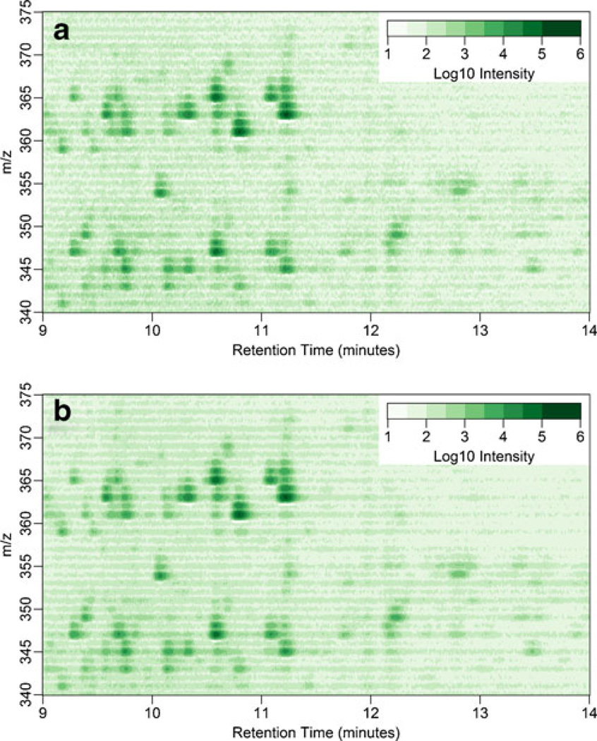
Our initial analysis evaluates a set of spectral profiles acquired from a single urine extract from a patient with Cushing’s disease. Figure 1 shows the spectral profile in the context of intensity. Figure 1a displays the intensity for a single replicate and Figure 1b is the arithmetic mean intensity of technical triplicates. From a cursory investigation, the spectral profiles look relatively identical. However, further inspection of the two shows that averaging triplicates reduces the background of the intensity plot. The isotopic cluster for cortisol (m/z=63.2, RT=11.2 min) can be discerned. Moreover, the in-source fragmentation product of Cortisol that results in [M − H₂O + H]⁺ =345.2 at RT=11.2 min can also be seen within this mass window. Since steroids are known to undergo dehydration in the ionization process, the prominent dehydration signal is not unexpected. Furthermore, examination of the plot for dehydration events is a useful strategy for identifying steroids with hydroxyl/ oxo moieties.

Figure 1.

Pseudocolor plots of mass spectral profile intensities of extracted urine from a Cushing’s disease patient. The plots include the m/z values 340–375 and RT of 9–14 min. Plots are of (a) the intensity of a single replicate and (b) the arithmetic mean intensity of technical triplicates of the same extract

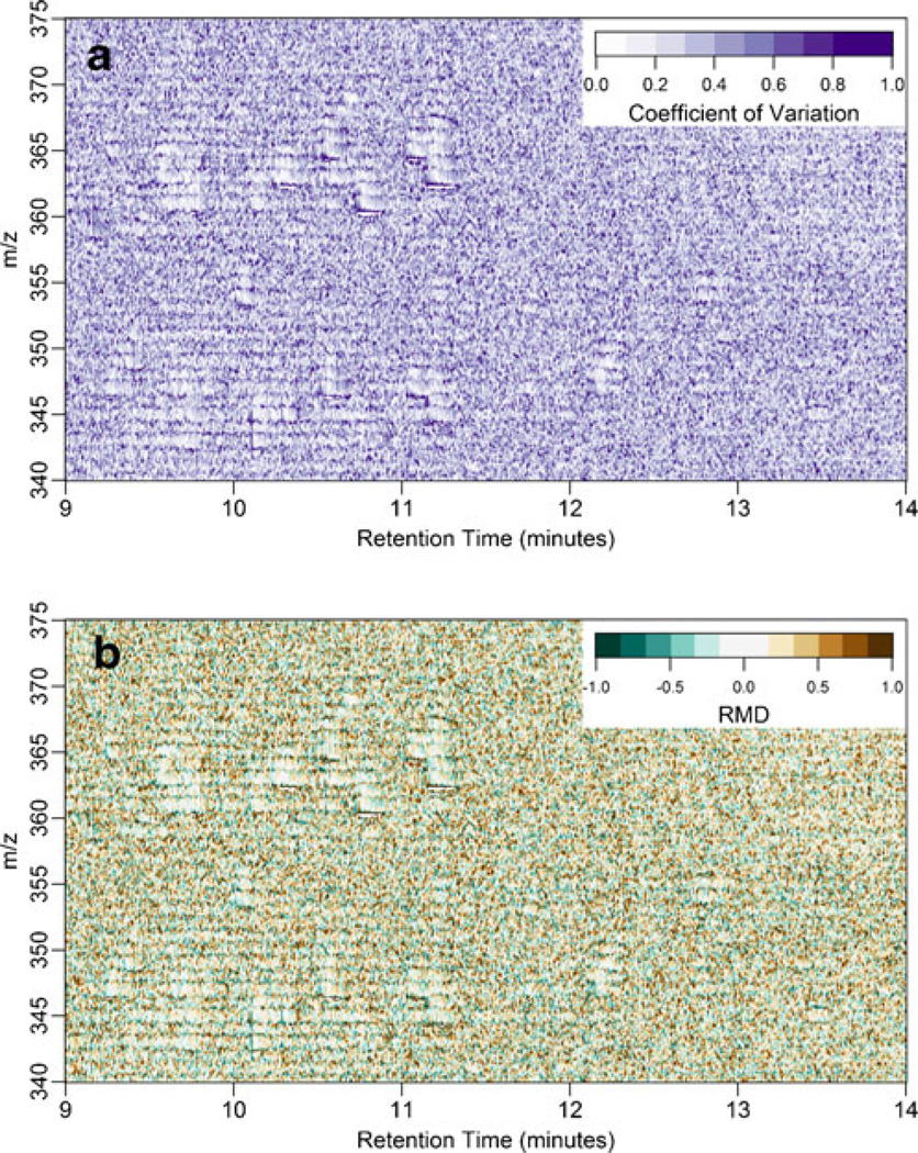
Using the three spectral profiles in Figure 1b, we were able to evaluate the quality of the replicate data. We examine the data quality in Figure 2 in two contexts: in Figure 2a we show the coefficient of variation of intensity values in the spectral profiles and in Figure 2b we show the RMDM. For these three replicates, regions of high signal (i.e., when analytes elute) generally have low variance (CV <0.2). Since these data are typically used without any preprocessing (e.g, de-isotoping, centroiding, or smoothing), they contain regions of high variance that would appear as halos around the elution of an analyte at the beginning of an isotope cluster as seen in Figure S1. A spectrum of such a region can be seen in Figure S2. This phenomenon is largely attributed to an artifact in the acquisition of signals near a high intensity ion. As a result of this artifact, we have chosen to “floor” the intensities of all signals for the figures in the main body of this text to an intensity of 30 counts; Figure S3 demonstrates how this value relates to the distribution of intensities in a single spectral profile. Following this correction, the “halo” region of high variance, Figure S1, transforms to a discrete area of 0.1m/z width where the intensity of the isotope cluster starts 0.1m/z earlier in a replicate relative to the other replicates, as seen in Figure 2b. To make this effect more apparent, we have included in Figure S1 subplots with higher floor values of 60 and 120 counts.

Figure 2.

Quality control pseudocolor plots of mass spectral profile intensities from extracted urine of a Cushing’s disease patient analyzed in technical triplicate. The plots include the m/z values 340–375 and RT of 9–14 mi. (a) A plot of the coefficient of variation of the intensity values, (b) A RMDM plot (see text for a description of this quantity)

Further evaluation of Figure 2b demonstrates a uniform spatial distribution of RMDM over the entire MRW except for those regions containing obvious peaks. These regions where peaks elute show minimal variation by virtue of their lack of color. Thus, RMDM is a convenient metric to evaluate data quality because it elucidates regions of high variation that may be skewed in the direction of their variance (i.e., heteroskedastic). The heteroskedasticity of mass spectral data highlights the utility of RMDM compared with CV; CV is not a signed quantity so it will be distributed around some value that cannot be known. Thus, while CV demonstrates variance, it cannot provide a metric for evaluating the fidelity of the data after a transformation such as flooring. In contrast, the RMDM is a signed quantity and should be centered on zero unless the data are floored improperly. In other words, this metric enables the analyst to assess regions of intensity that may have been recorded as spuriously high or spuriously low in a single replicate compared to other replicates. This could easily occur in a large randomized work list where one replicate injection has carryover from the previous injection whereas the other two replicates do not. This would result in locally high RMDM in the m/z region where the contaminant is observed, or broadly low RMDM in the circumstance of transient ion suppression.

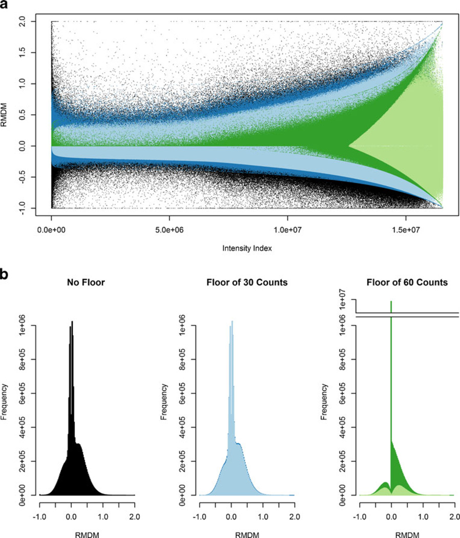
To demonstrate the importance of the floor value in data processing, we demonstrate the adverse effect of an excessively high value—60 counts compared with 30 counts—the value derived from the analysis of signal distribution in the data. The values of RMDM are plotted against a sorted intensity index in Figure 3a. Our conservative floor of 30 counts only alters ~3 % of the data, maintains both positive and negative RMDM values over the full range of intensities, and preserves the qualitative shape of the distribution seen in the unfloored data. On the other hand, the floor of 60 alters ~88 % of the data, removes the low intensity values that yield a negative RMDM, and distorts the distribution seen in the unfloored data. Figure 3b illustrates a more complete examination of the RMDM distributions under the different flooring conditions. Because of the small number of values altered, a floor of 30 counts preserves the distribution of the mass spectrometric signal (P=0.62, based on the Kolmogorov-Smirnov statistic). Additionally, this floor preserves distribution of variance regardless of how the values below the floor are treated; the distribution from the curve with the values removed (light blue) and set to the value of the floor (dark blue) do not differ significantly (P>0.99). When a floor of 60 counts is used, so much of the signal is altered that the distribution with values removed (light green) and with the values set at the value of the floor (dark green) differ significantly from the unfloored data (P<8E-10 and P<0.01, respectively). Because of the number of points affected by a floor of 60 counts, removing the intensities below the floor and setting them to the floor value produce different distributions (P< 6E-5). In short, the RMDM versus intensity index (Figure 3a) enable a subjective evaluation of how a flooring manipulation affects the shape of the variance; RMDM histograms (Figure 3b) and the Kolmogorov–Smirnov statistic provide a degree of objectivity in evaluating the effects of the chosen floor.

Figure 3.

RMDM distributions of spectral profile intensities from a urine extract from a Cushing’s disease patient analyzed in technical triplicate. The points in black have been plotted with no flooring. The values in blue have been floored to 30 counts. The values in green have been floored to 60 counts. The lighter hues are those values unaffected by flooring. These distributions are displayed both as (a) a scatter plot where the y-axis is RMDM and the x-axis is an intensity-sorted index and (b) as histograms

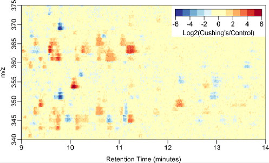
In addition to demonstrating a means for visualizing variance in replicates of full data sets, the approach we present also enables differential evaluation of data from independent specimens. A comparison of the arithmetic mean of technical triplicates of a Cushing’s disease urine extract and technical triplicates of a urine extract from a healthy control is shown in Figure 4. Note that the scale has been Log₂ transformed to emphasize the greatest differences between the diseased and normal test subjects as well as make each break in the color scale a Log₂ unit. The most intense values on the color scale are thus ≥32-fold higher in intensity. cortisol ([M + H]⁺ =363.2 and its dehydration product [M − H₂O + H]⁺ =345.2) can be seen at RT= 11.2 min and appear to have an average intensity ~8-fold increase, corresponding with elevated free cortisol expected in Cushing’s disease. In addition to cortisol, there appear to be at least eight other regions of intensity that indicate an increase in the concentration of unidentified analytes in the patient’s urine. The scope of this work intends to illustrate these visualization techniques and, as a result, we ultimately only confirm the identity of a single unknown analyte.

Figure 4.

A pseudocolor plot of the Log₂ transformed ratio of the arithmetic mean of intensities from mass spectral profiling of extracted urine from a Cushing’s disease patient and a healthy control. Each urine extract was analyzed in technical triplicate. The plot includes the m/z values 340–375 and RT of 9–14 min

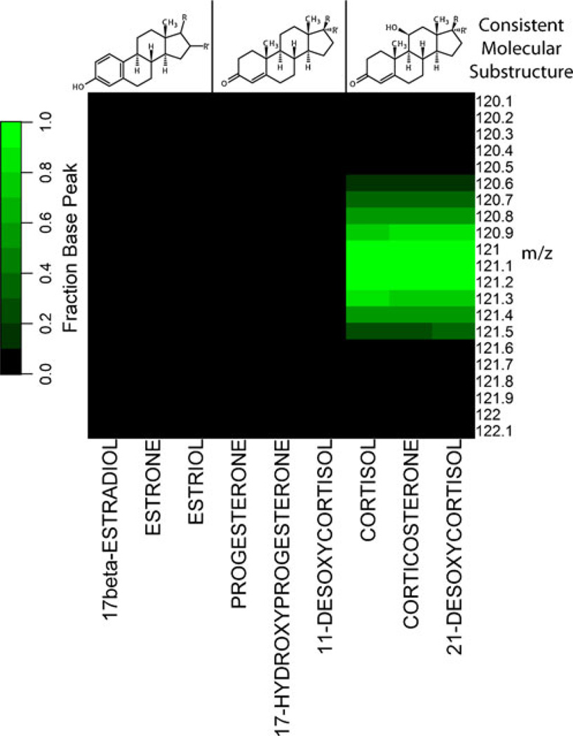
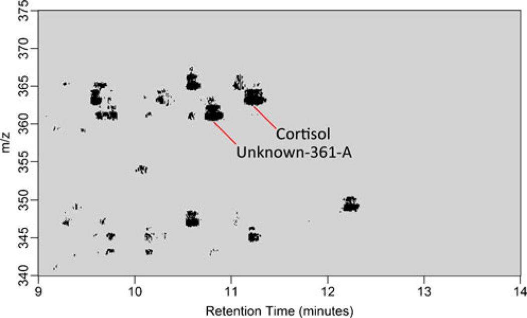
In the process of evaluating this ratiometric visualization plot it became apparent that we could leverage specific fragmentation products of steroidal classes to filter out features that belong to a particular steroidal subclass with the aim of identifying structurally similar compounds. By doing this, we could evaluate the relative concentrations of spectral features likely to be steroid hormones, but without necessarily relying on a standard MRM approach that requires a comprehensive library of chemical standards. We call this approach substructure-dependent analysis—it leverages the same understanding of gas phase chemistry of phospholipids [24]—but in the context of steroidal substructure. Those structural features that appear to most strongly dictate the fragmentation pattern of a steroid hormone are its A, B, and C ring configurations. Figure 5 shows the base-peak normalized product ion spectrum of nine steroid hormone standards from three different steroid hormone substructure classes at a CE of 40 eV. The fragment m/z= 121.1 is the base peak for all three steroid hormones containing the 4-ene-11-ol-3-one substructure. Conversely, the 4-ene-3-one and l,3,5(10)-triene-3-ol substructures produce this fragment at <10 % of the base peak of the product ion spectrum. We use this information to perform a set of precursor ion scans (m/z=121.1 for 4-ene-11-ol-3-one substructure, m/z=133.1 for 1,3,5(10)-triene-3-ol substructure, and m/z=109.1 for 4-ene-3-one substructure). The intensity values generated using this method are then compared with one another to examine when the diseased patient has a region of parent intensity elevated 4-fold over the control patient. We filter those regions of intensity by only those precursor ion scan values where the 4-ene-11-ol-3-one precursor ion scan intensity values are greater than the l,3,5(10)-triene-3-ol-dependent and 4-ene-3-one-dependent precursor scan intensity values. Application of this filtering method can be seen in Figure 6, where regions of elevated intensity that are 4-ene-11-ol-3-one substructure-dependent are colored black. We find it interesting that in addition to Cortisol, a number of the other elevated regions of intensity appeared to contain the 4-ene-11-ol-3-one substructure. We chose one of the areas of intensity (m/z=361.2, RT=10.8 min), denoted as unknown-361-A, to examine more closely. When considering its similarity to Cortisol in molecular substructure and retention time as well as its calculated double bond equivalents, we hypothesized that this compound was most likely cortisone. Comparison of this unknown-361-A’s product ion spectrum with that of cortisone and cortisol can be seen in Figure S4. We note that the base peak of the product ion spectrum of cortisone is m/z=163.1. Thus, this mode of analysis can be informative in guiding the investigator to the molecular substructure, but clearly there are other facets of the product ion spectrum of an unknown to consider before generating a structure (i.e., that the base peak of cortisone is 163.1 and not 121.1 suggests the oxidation of the hydroxyl in the C ring or some other modification in the A, B, and C ring substructure of cortisol).

Figure 5.

Evaluation of the product ion intensity as it relates to steroidal molecular substructure. The values are base peak normalized intensities of product ion spectra at CE=40 eV of pure standards. Green values are those m/z values of the product ion spectra that are ≥10 % of the base peak of the product ion spectrum of an analyte. Note that only those analytes that have the A, B, and C ring substructure of Cortisol produce a significant product ion at m/z= 121.1 at this collision energy

Figure 6.

A pseudocolor plot that shows substructure-dependent mass spectral profiling of extracted urine from a Cushing’s disease patient as it relates to a healthy control. The plot includes the m/z values 340–375 and RT of 9–14 min. The areas in black are regions where the technical triplicate arithmetic mean intensity of the Cushing’s disease urine extract is 4-fold greater than that of a healthy control and that the precursor ion scan intensity of the 4-ene-11-ol-3-one specific transition is greater than the 1,3,5(10)-triene-3ol or 4-ene-3-one specific transitions. Unknown-361-A was a mass spectral feature that did not exist in our initial set of standards and following further analysis was determined to be cortisone

While the approach we present here offers many attractive possibilities for novel data analysis, no amount of informatics can compensate for poor experimental design or performance. That is, the utility of this approach relies on a robust chromatographic method and a relatively stable signal from the mass spectrometer. On the other hand, evaluating the quality of data in a dataset this large (>10,000,000 points for a single spectral profile) can be a challenging exercise. This method demonstrates an approach to evaluating data quality in any LC/MS experiment that generates a large data set. Moreover, we have provided an approach to analysis of noise variance across an entire experiment. The greatest advantage to evaluating the noise across an entire dataset is the ability to intelligently select an intensity floor, as shown in Figure S3. The Figure shows a conservative cut-off can be made based on the inflection point from “zero” counts to the true baseline noise of the data. By making the cutoff in this way, while we have altered the distribution of ion intensity data, the fraction of signal points modified is less than 1 % of the total and we can demonstrate that those data were of no use in the subsequent analysis.

This computational workflow relies solely on the “raw” data to make decisions regarding spectral regions of interest. This reliance on the data itself rather than upon the extraction of predetermined features of one kind or another is the main differentiation between this method and other contemporary methods of profile mass spectrometry data analysis (e.g., XCMS, MAVEN, etc.). These other software packages manipulate the data via smoothing, binning, and retention time alignment, manipulations that are essential for feature list generation. Unfortunately, the parameters used to perform these manipulations (coarseness of smoothing, size of bins, tolerance of retention time windows) are difficult to determine empirically. Users typically gauge the success of the parameter tuning by the number of features the software detects. In light of the computational complexity other software packages present, our approach is quite straightforward: define the comparison (cohort of patients versus control) and the MRW (focusing around the elution of an analyte of known interest) and look for regions of great intensity. Moreover, our method provides very straightforward tools for evaluating the quality of the results. Regions of high signal intensity (e.g., “true” features) should have low variance (as seen in the CV/RMDM plots). Issues that present complications in other methods of analysis (such as retention time alignment) will manifest themselves in these quality evaluations.

The method we present here is also qualitatively different than the other approaches previously developed for 2D visualization of LC-MS data. Namely, our presentation of the data leverages very specific color palettes that facilitate data analysis. In our presentations, we use the appropriate class of color palette to enhance the analysis. Intensity and CV are sequential values and, thus, use sequential color schemes. RMDM and the difference plot in Figure 4 are datasets that diverge from a central value (0 in both cases) and, thus, they use diverging color palettes. Lastly, the substructure-dependent plot uses a qualitative color scheme. As an extreme example of the misuse of color in this application, Figure S5 presents identical data used in Figure 1a, but with a palette swap from a “sequential” green color palette to a “qualitative” rainbow color palette. Obviously, this misuse of color can even emphasize regions of noise that would typically be de-emphasized using a rational color palette.

This approach does not abstract the analysis away from the regime of mass spectrometry qua mass spectrometry. All spectral features are retained in this approach. Other summary-based approaches bin commonly encountered fragmentation events such as sodium adduction and in-source dehydration. These events are easy to recognize in the type of 2D pseudocolor plot used here and provide, especially in the context of steroid hormone analysis, a first-pass guide for those spectral features that are of molecular interest. Nonetheless, further analysis of the product ion spectrum and consideration of double bond equivalents should be considered before generating putative structures. We anticipate that further examination of a greater number of substructure classes will enable more powerful molecular substructure discrimination. These approaches combined will provide new insight into the analysis of discovery-based small molecular mass spectrometry experiments.

Conclusions

Our approach to 2D visualization of mass spectral profiles has enabled us to rapidly and directly evaluate features of interest without preprocessing. This method not only enables intensity-based metrics of visualization but also enables the visualization of data quality (e.g., CV or RMDM). Moreover, it provides the user the ability to filter features of interest by known substructure; though our experiments leveraged our understanding of steroid hormone behavior in the gas phase, this approach could also be used to discriminate lipids by head group. Other structural features could be interrogated by other scanning modes, such as neutral loss for probing decarboxylation events.

This technique is unique in its ability to enable untargeted analysis using a triple quadrupole mass spectrometer, which has typically been relegated to targeted analyses. However, this approach is general and can be applied to any mass spectral data that have not been preprocessed, including high-resolution data. This tool should see use in cases where experts want to directly interrogate their data for features that may be missed from traditional processing/binning methods. It will also see use when non-experts want to enable collaborators to analyze their data in a gel-like context that is more familiar to biologists than a spectral trace.

References

- 1.Sturm M, Bertsch A, Gropl C, Hildebrandt A, Hussong R, Lange E, Pfeifer N, Schulz-Trieglaff O, Zerck A, Reinert K, Kohlbacher O. OpenMS—An open-source software framework for mass spectrometry. BMC Bioinforma. 2008;9:163. doi: 10.1186/1471-2105-9-163. [DOI] [PMC free article] [PubMed] [Google Scholar]
- 2.Khan Z, Bloom JS, Garcia BA, Singh M, Kruglyak L. Protein quantification across hundreds of experimental conditions. Proc. Nat. Acad. Sci. 2009;106:15544–15548. doi: 10.1073/pnas.0904100106. [DOI] [PMC free article] [PubMed] [Google Scholar]
- 3.Pluskal T, Castillo S, Villar-Briones A, Oresic M. MZmine 2: Modular framework for processing, visualizing, and analyzing mass spectrometry-based molecular profile data. BMC Bioinforma. 2010;11:395. doi: 10.1186/1471-2105-11-395. [DOI] [PMC free article] [PubMed] [Google Scholar]
- 4.Sugimoto M, Hirayama A, Ishikawa T, Robert M, Baran R, Uehara K, Kawai K, Soga T, Tomita M. Differential metabolomics software for capillary electrophoresis-mass spectrometry data analysis. Metabolomics. 2010;6:27–41. [Google Scholar]
- 5.Grigsby CC, Rizki MM, Tamburino LA, Pitsch RL, Shiyanov PA, Cool DR. Metabolite Differentiation and Discovery Lab (MeDDL): A new tool for biomarker discovery and mass spectral visualization. Anal. Chem. 2010;82:4386–4395. doi: 10.1021/ac100034u. [DOI] [PubMed] [Google Scholar]
- 6.Smith CA, Want EJ, O'Maille G, Abagyan R, Siuzdak G. XCMS: Processing mass spectrometry data for metabolite profiling using nonlinear peak alignment, matching, and identification. Anal. Chem. 2006;78:779–787. doi: 10.1021/ac051437y. [DOI] [PubMed] [Google Scholar]
- 7.Frank AM, Bandeira N, Shen Z, Tanner S, Briggs SP, Smith RD, Pevzner PA. Clustering millions of tandem mass spectra. J. Proteome Res. 2007;7:113–122. doi: 10.1021/pr070361e. [DOI] [PMC free article] [PubMed] [Google Scholar]
- 8.Benton HP, Wong DM, Trauger SA, Siuzdak G. XCMS2: Processing Tandem mass spectrometry data for metabolite identification and structural characterization. Anal. Chem. 2008;80:6382–6389. doi: 10.1021/ac800795f. [DOI] [PMC free article] [PubMed] [Google Scholar]
- 9.Tautenhahn R, Bottcher C, Neumann S. Highly sensitive feature detection for high resolution LC/MS. BMC Bioinforma. 2008;9:504. doi: 10.1186/1471-2105-9-504. [DOI] [PMC free article] [PubMed] [Google Scholar]
- 10.Hoffmann N, Stoye J. ChromA: Signal-based retention time alignment for chromatography-mass spectrometry data. Bioinformatics. 2009;25:2080–2081. doi: 10.1093/bioinformatics/btp343. [DOI] [PMC free article] [PubMed] [Google Scholar]
- 11.Hiller K, Hangebrauk J, JaÃàger C, Spura J, Schreiber K, Schomburg D. MetaboliteDetector: Comprehensive analysis tool for targeted and nontargeted GC/MS based metabolome analysis. Anal. Chem. 2009;81:3429–3439. doi: 10.1021/ac802689c. [DOI] [PubMed] [Google Scholar]
- 12.Lommen A. MetAlign: Interface-driven, versatile metabolomics tool for hyphenated full-scan mass spectrometry data preprocessing. Anal. Chem. 2009;81:3079–3086. doi: 10.1021/ac900036d. [DOI] [PubMed] [Google Scholar]
- 13.Biswas A, Mynampati KC, Umashankar S, Reuben S, Parab G, Rao R, Kannan VS, Swarup S. MetDAT: A modular and workflow-based free online pipeline for mass spectrometry data processing, analysis and interpretation. Bioinformatics. 2010;26:2639–2640. doi: 10.1093/bioinformatics/btq436. [DOI] [PubMed] [Google Scholar]
- 14.Cottret L, Wildridge D, Vinson F, Barrett MP, Charles H, Sagot M-F, Jourdan F. MetExplore: A web server to link metabolomic experiments and genome-scale metabolic networks. Nucleic Acids Res. 2010;38:W132–W137. doi: 10.1093/nar/gkq312. [DOI] [PMC free article] [PubMed] [Google Scholar]
- 15.Tautenhahn R, Patti GJ, Kalisiak E, Miyamoto T, Schmidt M, Lo FY, McBee I, Baliga NS, Siuzdak G. metaXCMS: Second-order analysis of untargeted metabolomics data. Anal. Chem. 2010;83:696–700. doi: 10.1021/ac102980g. [DOI] [PMC free article] [PubMed] [Google Scholar]
- 16.Melamud E, Vastag L, Rabinowitz JD. Metabolomic analysis and visualization engine for LC-MS data. Anal. Chem. 2010;82:9818–9826. doi: 10.1021/ac1021166. [DOI] [PMC free article] [PubMed] [Google Scholar]
- 17.Olson M, Epstein J, Sackett D, Yergey A. Production of reliable MALDI spectra with quality threshold clustering of replicates. J. Am. Soc. Mass Spectrom. 2011;22:969–975. doi: 10.1007/s13361-011-0097-9. [DOI] [PubMed] [Google Scholar]
- 18.Sugimoto M, Kawakami M, Robert M, Soga T, Tomita M. Bioinformatics Tools for mass spectroscopy-based metabolomic data processing and analysis. Curr. Bioinforma. 2012;7:96–108. doi: 10.2174/157489312799304431. [DOI] [PMC free article] [PubMed] [Google Scholar]
- 19.R Development Core Team. R: A Language and environment for statistical computing. Austria: R Foundation for Statistical Computing, Vienna; 2010. [Google Scholar]
- 20.Fischer B, Neumann S, Gatto L. [Accessed 19 December 2011];mzR: parser for netCDF, mzXML, mzData and mzML files (mass spectrometry data) 2011 Available from: http://www.bioconductor.org/packages/release/bioc/html/mzR.html.
- 21.Wickham H. Reshaping data with the reshape package. J. Stat. Softw. 2007;21:1–20. [Google Scholar]
- 22.Brewer CA. Basic mapping principles for visualizing cancer data using geographic information systems (GIS) Am. J. Prev. Med. 2006;30:S25–S36. doi: 10.1016/j.amepre.2005.09.007. [DOI] [PubMed] [Google Scholar]
- 23.Advanced Chemistry Development Inc. ACD/ChemSketch Freeware. Canada: Toronto, ON; 2010. [Google Scholar]
- 24.Xia Y-Q, Jemal M. Phospholipids in liquid chromatography/mass spectrometry bioanalysis: Comparison of three tandem mass spectro-metric techniques for monitoring plasma phospholipids, the effect of mobile phase composition on phospholipids elution and the association of phospholipids with matrix effects. Rapid Commun. Mass Spectrom. 2009;23:2125–2138. doi: 10.1002/rcm.4121. [DOI] [PubMed] [Google Scholar]
Associated Data
This section collects any data citations, data availability statements, or supplementary materials included in this article.