Abstract
Background
The negative effects of X-ray exposure, such as inducing genetic and cancerous diseases, has arisen more attentions.
Objective
This paper aims to investigate a penalized re-weighted least-square (PRWLS) strategy for low-mAs X-ray computed tomography image reconstruction by incorporating an adaptive weighted total variation (AwTV) penalty term and a noise variance model of projection data.
Methods
An AwTV penalty is introduced in the objective function by considering both piecewise constant property and local nearby intensity similarity of the desired image. Furthermore, the weight of data fidelity term in the objective function is determined by our recent study on modeling variance estimation of projection data in the presence of electronic background noise.
Results
The presented AwTV-PRWLS algorithm can achieve the highest full-width-at-half-maximum (FWHM) measurement, for data conditions of (1) full-view 10mA acquisition and (2) sparse-view 80mA acquisition. In comparison between the AwTV/TV-PRWLS strategies and the previous reported AwTV/TV-projection onto convex sets (AwTV/TV-POCS) approaches, the former can gain in terms of FWHM for data condition (1), but cannot gain for the data condition (2).
Conclusions
In the case of full-view 10mA projection data, the presented AwTV-PRWLS shows potential improvement. However, in the case of sparse-view 80mA projection data, the AwTV/TV-POCS shows advantage over the PRWLS strategies.
Keywords: X-ray computed tomography, low-mAs protocol, penalized re-weighted least-squares, adaptive weighted total variation, projection onto convex sets
I. Introduction
X-ray computed tomography (CT) has demonstrated dramatic impact on medical imaging over the last several decades. However, due to the thousands of projection views in normal scan, high X-ray radiation exposure in clinic has caused potential cancer risks to the patients [1]. Therefore, minimizing the radiation risks is strongly desirable in the CT field. Up to now, besides hardware-based optimal data-acquisition protocols [2–4], two types of data acquisition for reducing the radiation dose have been widely explored, i.e., (1) reducing the number of projection views [5, 6] and (2) reducing the milliampere-seconds (mAs) or the kilovoltage-peak (kVp) values [7–9].
Reducing the number of projection views per rotation around the body, which is called sparse-view scanning nowadays, can directly reduce the radiation dosage, but the associated image reconstruction is ill-posed for the well-known Feldkamp–Davis–Kress (FDK) method [10] due to the insufficient measurements. Recently, compressed sensing (CS) theory has proved that an image can be uniquely reconstructed from far less measurements than the required data of Nyquist sampling theorem if the transform coefficients of the data are sparse enough [11]. Meanwhile, due to the property of CT projection data, it is difficult to adopt the CS theory directly for CT image reconstruction [12]. Inspired by the preliminary idea of CS, the total variation-projection onto convex sets (TV-POCS) [5, 6] method and its generalized case: adaptive-weighted total variation-projection onto convex sets (AwTV-POCS) [12] method, have been proposed for solving the CT image reconstruction from sparse-view measurements. In our previous study on AwTV-POCS method, we observed gains at the edges of the reconstructed image compared to the conventional TV model [12]. In addition, to further reduce the number of projection views without corrupting the image quality, a prior image constrained compressed sensing (PICCS) strategy has been proposed [13]. A drawback to all these TV-based methods mentioned above is that they do not fully consider the statistical property of the projection data. More reasonable data fidelity metric between the measured and desired projection data is demanded to make the feasible region small enough. Otherwise, it may be difficult to find an optimal solution close enough to the true one. Hence, in the construction of objective function of the TV-based methods, considering the statistical property of projection data would significantly improve the associated performances.
Reducing the X-ray exposure (i.e., lowering the mAs or kVp values) to the patients is another direct strategy for lower the radiation dose [8]. However, the image quality in this case would be significantly degraded due to excessive quantum noise if no noise controlling [14, 15]. Efforts have been devoted to restore the ideal line integrals or sinogram data (i.e., projection data after log-transformation) from the acquired low-mAs projection data for the purpose of improving the image quality via either statistics based sinogram restoration [7–9] or statistics based iterative image reconstruction [16–19]. For yielding a successful solution, the AwTV penalty [12] is introduced in the objective function by considering both piecewise constant property and local nearby intensity similarity of the desired image, which is one of motivations for this present study. The differences between the two penalties (i.e., AwTV and TV) will be discussed in this paper. In addition, previous statistical model in the image reconstruction algorithms does not consider the electronic background noise. As far as we know, there are two principle sources of causing the CT noise, i.e., photon counting statistics and the electronic background noise [19]. Thus, more accurate model with consideration of the electronic noise is desired for statistical image reconstruction (SIR), which is the other motivation of this present study. It is worth to note that the penalty term and the explored statistical model in this study differentiate the ones from the previous reports on TV-PWLS (penalized weighted least squares) [20–24].
The remainder of this paper is organized as follows. In Section II, the proposed penalized re-weighted least squares (PRWLS) image reconstruction strategy based on a new accurate noise model of projection data and the AwTV penalty are first described, and then a modified Gauss-Seidel iterative update strategy is introduced for solving the objective function of AwTV-PRWLS. Additionally, a brief outline of experimental design is illustrated to validate the present algorithm using cone-beam CT (CBCT) measurements from the CatPhan® 600 and anthropomorphic head phantoms. In Section III, experimental results from two phantoms are reported. Finally, discussions and conclusions are given in Section IV.
II. Methods and Materials
II.A. AwTV prior
Borrowing the mathematical descriptions presented in the reference [12], the three-dimensional (3D) AwTV prior of can be written as:
| (1) |
| (2) |
where s and t are the indices of the location of the attenuation coefficients along in-plane domain (slice), z is the indices of the attenuation coefficients along axial direction, δ in the weights is a scale factor which controls the strength of the diffusion during each iteration. Intuitively, the AwTV model of Eq. (1) approaches to the conventional TV prior model as the weight goes to 1, thus the TV prior model may be considered as a special case of the AwTV model when δ → ∞. Extensive experiments have shown that the effectiveness of the AwTV prior model in sparse-views CT image reconstruction [12].
II.B. PRWLS image reconstruction
According to our knowledge, Compound Poisson model [25] can accurately describe the noise property of the detected photon numbers in CT scanners based on the energy spectrum of the X-ray quanta. However, it is numerically difficult to directly implement this model for data noise simulation. Several reports have discussed approximation of this model by the Poisson model [9, 16, 23, 25, 26]. Practically, the measured transmission data I can be assumed to statistically follow the Poisson distribution upon a Gaussian distributed electronic background noise [19]:
| (3) |
where λ is the mean of Poisson distribution, me and are the mean and variance of the Gaussian distribution from the electronic background noise. In reality, the mean me of the electronic noise is often calibrated to be zero (i.e., ‘dark current correction’) and the associative variance slightly changes due to different settings of tube current, voltage and durations in a same CT scanner [19]. Hence, in a single scan, the variance of electronic background noise can be considered as uniform distribution. Based on this measurement model, a new formula of the mean-variance relationship in CT projection domain by considering the effect of the Gaussian distributed electronic background noise has been reported as follows [19]:
| (4) |
where represents the estimated variance of measuring projection datum pi, Ii0 is the mean number of incident photons along projection path i, p̄i denotes the mean of the log-transformed ideal projection datum pi along path i, is the variance of the electronic noise associated with the measurement on projection datum pi, which can be obtained from the mAs levels versus variance of the electronic noise curve [19].
From Eq. (4), it can be observed that a larger p̄i value, indicating less X-ray photons being detected in the detector, will have a larger variance. Thus, a smaller signal-to-noise ratio (SNR) is expected due to the Poisson noise nature of the detected photons. On the contrary, a smaller p̄i value will result in a higher SNR. Due to this property, the inverse of the in Eq. (4) shall be used as the weights for the weighted least squares (WLS) term, i.e., a lower SNR shall contribute less for the estimate of the ideal projection and a higher SNR will contribute more for the estimation. This expectation is proved mathematically by Taylor expansion on the signal model (3) [19]. In reality, the images are reconstructed from only one scan and the mean line integral p̄i are not available (actually it is to be estimated). Therefore, a one-step-later reweighted strategy was implemented to estimate from the measured projection data [18]. This strategy makes sense that the re-projection operations from the reconstructed image are much closer to the mean of the ideal log-transformed projection.
For CT image reconstruction, using the terminologies described in the previous study [8], the associated cost function of PRWLS can mathematically be written as:
| (5) |
where p̂ is the acquired projection data and A represents the system transfer matrix, which depends on the projection geometry, and its elements of ai,j can be calculated as the length of the intersection of projection ray i with voxel j, μ is the vector of ideal attenuation coefficients. The first term on the right hand side is named as the data fidelity term described as a re-weighted least-squares or RWLS measurement wherein the matrix Σ, which is a diagonal matrix and whose i-th element denotes the variance of the projection datum at detector i as defined by Eq. (4). Directly minimizing the RWLS measure, similar to the maximum-likelihood (ML) approach, usually leads to unacceptable results [9]. Thus, a penalty R(μ) (the second term in the right hand side of Eq. (3)) is often desired for a successful solution. The hyper-parameter β > 0 is designed to control the strength of the penalty term R(μ) in Eq. (5). Consequently, the desired image can be yielded by solving the following objective function:
| (6) |
As for the selection of penalty term R(μ), many forms have been explored as an a priori constraint to regularize the RWLS solution, such as the isotropic quadratic prior [8] and anisotropic quadratic prior [18], by attempting to adapt different weighting coefficients under the framework of Markov Random Field (MRF). Recently, based on the hypothesis of the piecewise constant property of the to-be-estimated image, several TV-based prior models [5, 6, 21] were proposed for CT image reconstruction. However, these models often suffer over-smooth in the cases of the desired images containing low-contrast edges. To address the drawback of TV-based prior models, an AwTV prior model was introduced by our group recently [12] for sparse-views CT image reconstruction with significant gains than the conventional TV model in terms of edge details preservation. In this study, the AwTV prior model as described in last section was used for CT image reconstruction. For simplicity, the present CT image reconstruction strategy is named as the AwTV-PRWLS.
II.C. Implementation of the AwTV-PRWLS method
By incorporating the AwTV prior in Eq. (5), the objective function of the AwTV-PRWLS method for CT image reconstruction can be written as:
| (7) |
Generally, to yield a unique convergence solution, the convexity of the objective function in Eq. (7) should be considered. It can be easily observed that the data fidelity term in Eq. (7) has a convex quadratic form while the associated AwTV prior term is not convex due to the nonlinear distribution about the local intensity of the image. Hence, it is difficult to get a global optimal solution from Eq. (7) directly. Meanwhile, inspired by the optimization strategy as described in the previous works [18, 27], the weights can be pre-calculated separately before each iteration step and given the pre-calculated weights the convex of AwTV prior term can be well achieved. As a result, through a traditional optimization algorithm performing on the objective function in Eq. (7), at least one local convergence solution can be generated. Practically, the estimated image after several iterations would convergence to a stable one with only minor changes of intensity, which means that the weights almost unchanged after several iterations. In other words, a converged solution always can be yielded by the optimization method as described in the previous works [18, 27]. In this study, based on the previous works in SIR [18, 22, 28], a modified Gaussian Seidel (GS) update strategy was performed on the optimization of the objective function in Eq. (7). It should be mentioned, because the weights are pre-calculated before each iteration and are considered as constants in each iteration, the minimizing of AwTV penalized cost function should have similar property as the TV penalized cost function [22]. To summarize, the pseudo-code of the present algorithm about the AwTV-PRWLS can be listed as follows:
| 1: | Initialization: |
| 2: | μ̂ = FDK {p̂}; |
| 3: | r̂ = p̂ Aμ̂; |
| 4: | , i =1, 2,… M; |
| 5: | , ∀j; |
| 6: | , m ∈ Nj; |
| 7: | For each iteration: |
| 8: | For each pixel j ={s, t, z}: |
| 9: | For each neighbor m ∈ Nj |
| 10: | if m ∈ M = {s−1, t, z} ∪ {s, t−1, z}∪{s, t, z−1} |
| 11: | ; |
| 12: | if m ={s+1, t, z}, |
| 13: | |
| 14: | else if m ={s, t+1, z}, |
| 15: | ; |
| 16: | else if m ={s, t, z+1}, |
| 17: | ; |
| 18: | end if |
| 19: | ; |
| 20: | ; |
| 21: | ; |
| 22: | ; |
| 23: | end for |
| 24: | end for |
| 25: | update , m ∈ Nj; |
| 26: | update , i =1, 2,…M, where p̃ = Aμ̂; |
| 27: | end if stop criterion is satisfied. |
where aj denotes the column vector of the system matrix A, are the weights for the neighboring voxels m, which are updated in each iteration, ε is a relax parameter introduced to avoid the denominator going to zero, M is the total projection ray numbers. In line 2, an initial estimate of the to-be-reconstructed image is set to be the result of FDK. The initial estimation of the variances of measuring projection data for i=1…M are calculated from the acquired projection data. And according to the result of FDK, the anisotropic weights are initialized in line 6. From line 8 to line 24, each pixel is updated continuously by the GS strategy. By incorporating the weights or the neighboring voxels, an updating equation is performed at line 20. Then the anisotropic weights are updated based on new estimated intensities of voxels after one iteration at line 25. The variances of measuring projection data are also updated based on the re-projected measurements from the new intensities at line 26. It is worth to note that by setting the anisotropic weight to 1, the above pseudo-code for the present AwTV-PRWLS algorithm corresponds to the TV-PRWLS algorithm [22]. The final results will be obtained as the stop criterion condition is met as indicated at line 27. Specifically, in this study, the value of mean square error (MSE) between the results from the current iteration and the previous iteration is used as the stop criterion. The convergence analysis of the present AwTV-PRWLS algorithm would be shown in Section III.A.3.
II.D. Data acquisition
To calculate the variance of the projection data, the mean number of incident photons along projection path i should be estimated according to Eq. (4). It is known that the incident photon number is mainly determined by the protocols of the tube current and the duration of X-ray pulse. Ideally, the incident photons should be uniformly distributed across the field of view (FOV). However, considering the concavity of the human body, a bow-tie attenuation filter is often installed between the human body and the X-ray source [29], which makes the incident photons across the FOV no longer uniform. To accurately estimate the incident intensity over the FOV at a specific mAs level, an air scan was first performed at the same mAs level. Figure 1 shows an example of the incident X-ray intensity in low-mAs case acquired by ExactArms (kV source/detector arms) of a Trilogy™ treatment system (Varian Medical Systems, Palo Alto, CA) [29] by averaging the projections of one circle rotation. For the low-mAs case, the X-ray tube current was set at 10mA and the duration of the X-ray pulse at each projection view was set to be 10 ms. For the corresponding normal-mAs case, the tube current was set at 80mA and the duration of the X-ray pulse at each projection view was 12 ms. In this study, the tube voltage was all set to be 125 kVp for all the cases.
Fig. 1.

Incident X-ray intensity image across the field of view with 10 mA tube current and 10 ms pulse time in cone-beam geometry.
The CBCT projection data acquired by the same CT system from two physical phantoms (i.e., the CatPhan® 600 and anthropomorphic head phantoms) were used to evaluate the performance of the above presented AwTV-PRWLS algorithm in this study. A total of 634 projection views were acquired for a fully 360-degree rotation on a circular orbit. The dimension of each projection image is 1024×768 pixels. To reduce computational time, the projection data were down-sampled by a factor of 2. Only 8 out of 768 slices from the projection image were selected for image reconstruction. The source-to-isocenter distance is 100 cm and the source-to-detector distance is 150 cm. The array size of the reconstructed image is 350×350×8 and the associative voxel size is 0.776×0.776×0.776 mm3. Sparse-view projection data are extracted evenly over 360 degrees from full projection views for further analysis.
II.E. Image quality measures
One of the most important merits for medical image evaluation is the resolution. The high resolution image delivers clear messages to the physicians for diagnoses; the low resolution image loses some small features, which is more dangerous for clinical image. However, mitigating the artifacts from noise or missing data due to the reduction of X-ray exposure while maintaining good structure information is more challenging for the general CT image reconstruction methods. To quantitatively describe the resolution level of the reconstructed image, the full-width-at-half-maximum (FWHM) is always calculated for evaluation purpose. In order to obtain an FWHM value, a Gaussian-like function is used to fit the edge spread function (ESF) or an impulse response in the reconstructed image. Through those fitted curves, it can be observed the high-resolution image will often have a higher peak value and low-resolution image often has a lower peak value. To quantize this observation, the FWHM values of the fitted Gaussian broadening kernel are calculated by 2.35σR, where σR is the standard deviation of the Gaussian broadening kernel [12]. Then, high resolution image will have a smaller FWHM value and low contrast image will have a larger FWHM value.
Beside the merit of FWHM value, another merit – the noise level of the desired image is also very important for diagnosis. The physicians are hardly to locate the polyp from a noisy image. To quantitatively describe the noise level of the image, a uniform area (i.e., region-of-interest (ROI)) is always been selected to calculate the standard deviation. The smaller standard deviation indicates the image has a low-level noise, and a higher standard deviation indicates a noisy image is obtained. Then, if we combine the resolution (i.e., FWHM value) with the noise level merit, we can draw a curve to describe the trade-off between them, which will indicate the performance of image reconstruction algorithms. We call this curve as resolution-noise trade-off curve. The curve of an outstanding algorithms will very close to the original point, which indicates a high resolution and low noise level result image sill be generated.
Besides those two merits, the convergence analysis for an image reconstruction algorithm is necessary. A stable algorithm will always ensure the results converge to a global minimum. In the following section of results, we will focus our study on these three merits.
III. Results
In this study, two physical phantoms (i.e., CatPhan® 600 phantom and Anthropomorphic Head phantom) were utilized for evaluation. For each physical phantom, three type of data: (1) full-view 10mA projection data; (2) sparse-view 80mA projection data; and (3) sparse-view 10mA projection data were studied. Table I shows the methods as used in this section. To compare the impact of the priori model (i.e., penalty term), the AwTV-PRWLS were compared to TV-PRWLS for different parameters. To compare the influence of the variance estimation model of projection on the PRWLS method, the proposed AwTV/TV-PRWLS were compared to the AwTV/TV penalized uniform weighted least-squares strategy (AwTV/TV-PUWLS), which uses uniform weights in the statistical part (i.e., Σ was equal to identity matrix in Eq. (7)). In addition, to validate the statistical model, the proposed AwTV/TV-PRWLS were compared to the AwTV/TV-POCS methods.
Table I.
Description of three methods
| Name | Formula |
|---|---|
| AWTV/TV-PRWLS | ; |
| AWTV/TV-PUWLS | ; |
| AWTV/TV-POCS | ; |
III.A. CatPhan® 600 phantom study
III.A.1. Influence of the priori model on the PRWLS method
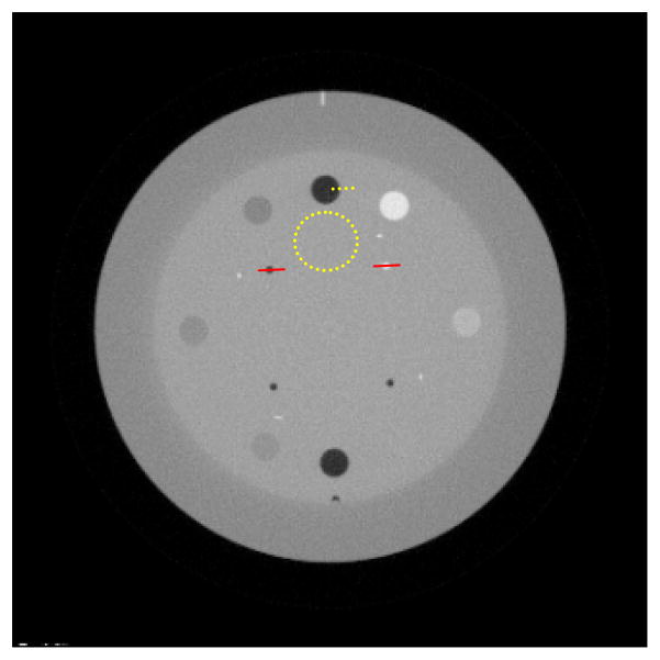
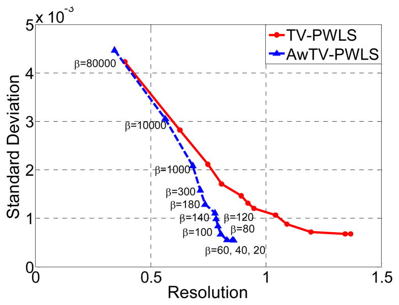
To investigate the effects of the two prior models, i.e., TV and AwTV model, the full-view 10mA data was utilized for this study. The resolution of the resulting image was calculated from the edge spread function (ESF) along the horizontal profile as indicated by the yellow dot lines on the top cold circle shown in Fig. 2. In addition, a small region is selected as indicated by the yellow dot circle in Fig. 2 to calculate the standard deviation σN. By varying the penalty parameter β from 20 to 8 × 10⁴, we can obtain two resolution-noise tradeoff curves in the coordinates (2.35σR, σN) for the TV-PRWLS and AwTV-PRWLS algorithms with δ = 0.006 as shown in Fig. 3.
Fig. 2.
The reconstructed transverse image of the CatPhan® 600 phantom from full-view normal-mAs projection data.
Fig. 3.
The resolution-noise tradeoff curves of the transverse reconstructed images of the CatPhan® 600 phantom by the TV-PRWLS and AwTV-PRWLS algorithms.
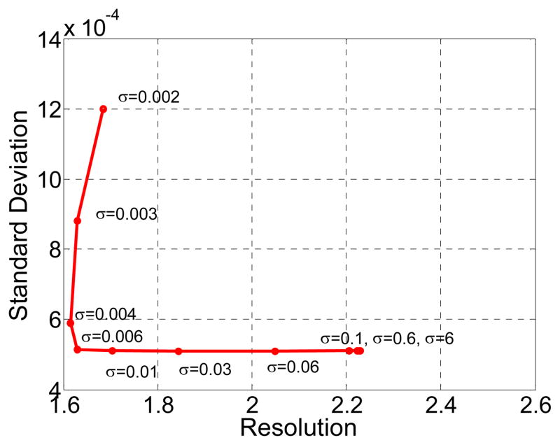
From Fig. 3, it can be observed that the result of AwTV-PRWLS algorithm has a higher resolution compared to the TV-PRWLS algorithm at the same noise level. In addition, a better balance between the noise and resolution can be observed as β = 140. In order to further validate the effects of parameter δ in the adaptive weights to the resulting image, a group of resolution-noise pairs were calculated towards the different δ values from 0.002 to 6 at β = 140 as shown in Fig. 4.
Fig. 4.
The resolution-noise tradeoff curve of the transverse reconstructed images of the CatPhan® 600 phantom by the AwTV-PRWLS algorithm with different δ values from 0.002 to 6.
As shown in Fig. 4, the resolution-noise tradeoff curve indicates that the reconstructed image by the AwTV-PRWLS algorithm has both good resolution and lowest noise level with δ = 0.006 for the CatPhan® 600 phantom study. Moreover, it should be mentioned that as the value of δ decreases from 0.006 to 0.002, the noise level (i.e., standard deviation) increases noticeably from 5.0818 × 10⁻⁴ to 1.2 × 10⁻³, and the associative resolution of the image decreases a little from 1.6293 to 1.6842. At the same time, as the value of δ increases from 0.006 to 6, the noise still maintains at a lower level while the resolution drops noticeably from 1.6293 to 2.2292 and finally locates at a fixed value when δ approaches a very large one. This result is consistent with our previous comparison study on the AwTV-POCS and TV-POCS [12] algorithms where the additional adaptive weights in the AwTV model show good property to preserve edges while mitigating noise of the resulting image.
III.A.2. Influence of the variance estimation model of projection on the PRWLS method
III.A.2.1 Visualization-based comparison
In this section, 79 projection views are extracted from the 80mA and 10mA projection data to generate type (2) and type (3) datum. Thus, the associative dosage can reduce to about 1/9, 1/8, and 1/72 of the dosage of full-view 80mA data, respectively. As for the comparison with the present AwTV-PRWLS, other three methods, i.e., the TV-PRWLS, AwTV- and TV-PUWLS were explored in this study. In the implementations, due to that a standard deviation can reflect the noise level of the to-be-reconstructed image, a ROI as indicated by the circle in was selected from the uniform background in the phantom to calculate standard deviation. To mitigate the effects caused by different parameter selection, different values of β were selected to keep the resulting images having the same noise level described by a standard deviation. Specifically, for the AwTV/TV-PRWLS methods, β =140 for all three types of data; for the AwTV/TV-PUWLS methods, β =5000.
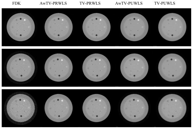
A reconstructed slice of the CatPhan® 600 phantom is shown in Fig. 5. The first row of Fig. 5 is the results reconstructed from type 1 (i.e., full-view 10mA projection) data by the FDK and AwTV/TV-PRWLS and AwTV/TV-PUWLS methods. The second and third rows of Fig. 5 are the results reconstructed from type 2 (i.e., 79-view 80mA projection) data and type 3 (i.e., 79-view 10mA projection) data. It can be seen that the FDK method cannot produce satisfied results in all the cases. In addition, the AwTV/TV-PRWLS methods achieve significant gains than the AwTV/TV-PUWLS methods in terms of noise suppression and resolution preservation. Small differences are also observed between the results from the AwTV-PRWLS and TV-PRWLS methods due to different penalty term settings. The related further discussion can be found in the following section.
Fig. 5.
The reconstructed images of the CatPhan® 600 phantom. The first row shows the images reconstructed from the full-view 10mA projection data. The second row shows the images reconstructed from the 79-view 80mA projection data. The third row shows the images reconstructed from the 79-view 10mA projection data. The display window is [0, 0.03].
III.A.2.2 Profile-based comparison
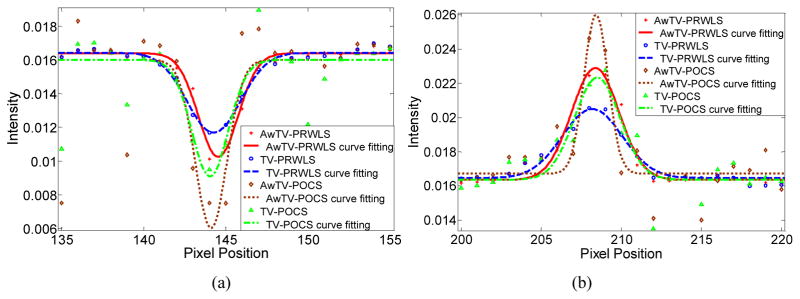
Figures 6, 7 and 8 show the profiles passing through the two spots, as indicated by red line in Fig. 2, in the images reconstructed from three types of data, respectively. A Gaussian like function is used to fit the profiles as indicated in the figures. From Fig. 6, we can observe that in the case of full-view 10mA projection data, the peak values of the results from AwTV/TV-PRWLS are much higher than that from AwTV/TV-PUWLS in both cold and hot spots. We also observe the gains from our AwTV model compared to the conventional TV model. For the 79-view 80mA projection data case, the results are shown in Fig. 7. In the 79-view 10mA projection data case, shown in Fig. 8, although all the images are not acceptable (i.e., inferior results), we still observe some gains by using the AwTV-PRWLS frame work.
Figure 6.
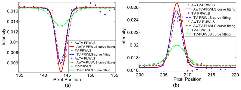
Horizontal profiles of the CatPhan® 600 phantom images reconstructed by different algorithms from full-view 10mA projection data. Picture (a) shows the profiles across the cold spot (146th row, 135th to 155th column). Picture (b) shows the profiles across the hot spot (139th row, 200th to 220th column).
Figure 7.
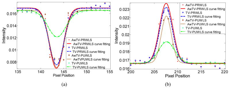
Horizontal profiles of the CatPhan® 600 phantom images reconstructed by different algorithms from 79-view 80mA projection data. Picture (a) shows the profiles across the cold spot (146th row, 135th to 155th column). Picture (b) shows the profiles across the hot spot (139th row, 200th to 220th column).
Figure 8.
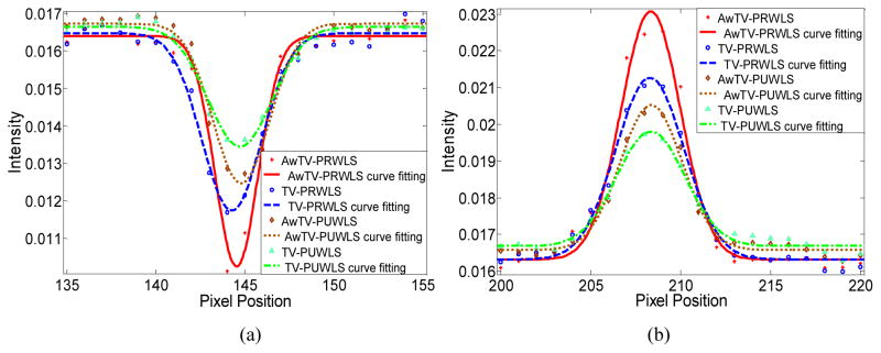
Horizontal profiles of the CatPhan® 600 phantom images reconstructed by different algorithms from 79-view 10mA projection data. Picture (a) shows the profiles across the cold spot (146th row, 135th to 155th column). Picture (b) shows the profiles across the hot spot (139th row, 200th to 220th column).
III.A.2.3. FWHM measures
To further quantitatively analyze the gains from the present PRWLS method than the PUWLS method, the FWHM of the two spots (a cold spot and a hot spot) are calculated and shown in Table II. The Table II reveals the AwTV/TV-PRWLS methods can produce smaller values than the AwTV/TV-PUWLS methods on both hot and cold spots, which is consistent with our observation about the profile comparison. It should be mentioned that the FWHM values of the cold spots in the results from 79-view 80mA projection data by AwTV-PUWLS has the smallest value than the other results. This apparent contradiction, however, is likely due to the curve fitting options which make the area under curve of the Gaussian-like bell shape are much smaller than others and can be illuminated by observing the curve fitting results shown in Fig. 7(b).
Table II.
The FWHM value of the cold and hot spots in Fig. 3
| Data type of projection | Position | AwTV-PRWLS | TV-PRWLS | AwTV-PUWLS | TV-PUWLS |
|---|---|---|---|---|---|
| Full-views 10mA | cold spot | 4.7470 | 4.7565 | 4.8222 | 5.7763 |
| hot spot | 4.6836 | 4.9891 | 4.9749 | 6.0207 | |
| 79-views 80mA | cold spot | 5.0455 | 5.0689 | 5.2241 | 6.3967 |
| hot spot | 4.4650 | 4.4979 | 3.5885 | 5.7085 | |
| 79-views 10mA | cold spot | 3.9222 | 5.3275 | 5.3181 | 6.0419 |
| hot spot | 5.4802 | 6.1406 | 5.7246 | 6.3215 |
III.A.3. Convergence analysis of the AwTV-PWLS algorithm
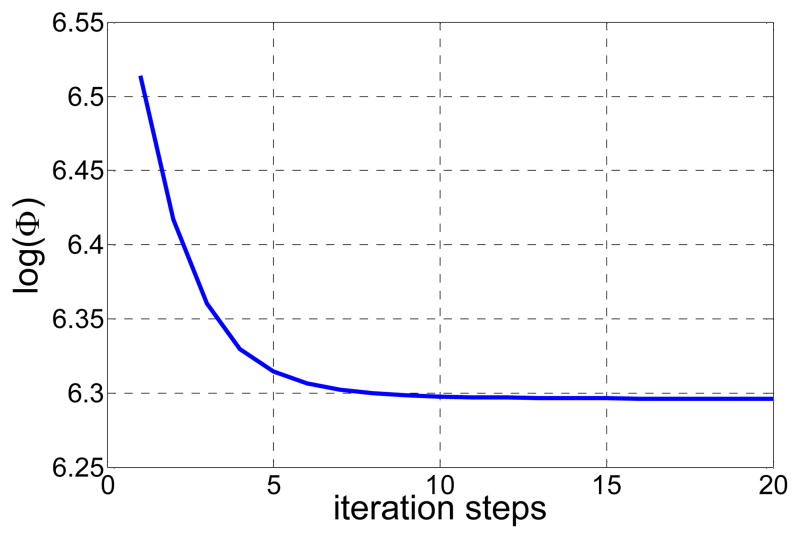
The convergence property of the AwTV-PRWLS algorithm was documented by calculating the value of cost function Φ for the full-view 80mA projection CatPhan® 600 phantom data. Figure 9 shows the value of log(Φ) versus the iteration steps for the AwTV-PRWLS algorithm. We can observe that the value of Φ decreases monotonously as the number of iteration steps increases. Finally, we found the objective value arrived at a stable value at the 20th iteration and we believe the algorithm has converged sufficiently and the to-be-estimated image would only have tiny changes (hardly be observed by human eye) for further iteration.
Fig. 9.
Convergence analysis: log(Φ) v.s. iteration steps.
III.A.4. Comparisons of the AwTV/TV-PRWLS and AwTV/TV-POCS methods
III.A.4.1 Visualization-based comparison
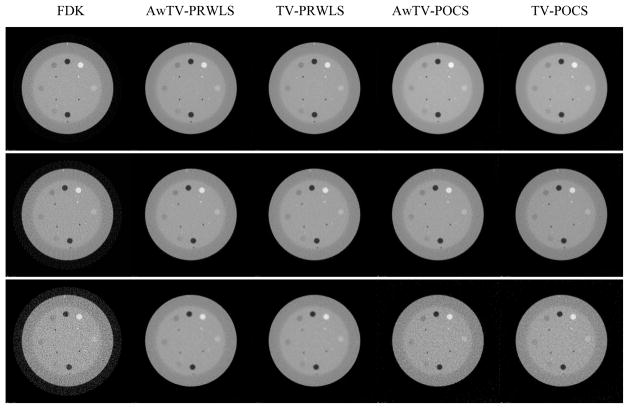
According to our previous study [12], the AwTV/TV-POCS algorithms show satisfactory results for image reconstruction from sparse-view 80mA projection data. To further validate the two types of strategy (i.e., the POCS and PRWLS) for different types of projection data measurements (i.e., low-mAs data or sparse-view data), the AwTV/TV-PRWLS and AwTV/TV-POCS algorithms were implemented to reconstruct three types of data as mentioned in previous section. In the AwTV/TV-PRWLS strategies, the penalty parameter β was selected to be 140 to ensure the backgrounds have similar noise levels as the full-view 80mA FDK image. For the AwTV/TV-POCS approaches, five POCS steps and two TV gradient descent steps [5, 6, 12] were executed in each general loop to achieve the results with similar noise level. The results are shown in Fig. 10.
Fig. 10.
The reconstructed images of the CatPhan® 600 phantom. The first row shows the images reconstructed from the full-view 10mA projection data. The second row shows the images reconstructed from the 79-view 80mA projection data. The third row shows the images reconstructed from the 79-view 10mA projection data. The display window is [0, 0.03].
III.A.4.2 Profile-based comparison
To further compare the reconstructed images, the profiles and FWHM values were calculated as shown in Figs. 11–13. Figure 11 indicates that the results from AwTV/TV-PRWLS have higher peak values on both spots indicating better performance on edge preserving for full–view 10mA projection data. Figure 12 indicates that the results from AwTV/TV-POCS have higher peak values on both spots for 79-view 80mA projection data. Obviously, in the 79-view 10mA projection data case, it is difficult to make any confidential conclusion for the inferior results. Although we observe the AwTV/TV-POCS shows some improvement to the AwTV/TV-PRWLS, the background noise is much higher than the results from AwTV/TV-PRWLS.
Figure 11.
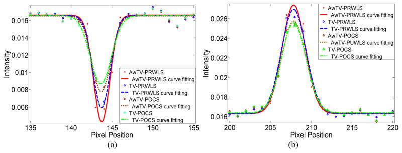
Horizontal profiles of the CatPhan® 600 phantom images reconstructed by different algorithms from full-view 10mA projection data. Picture (a) shows the profiles across the cold spot (146th row, 135th to 155th column). Picture (b) shows the profiles across the hot spot (and 139th row, 200th to 220th column).
Figure 13.
Horizontal profiles of the CatPhan® 600 phantom images reconstructed by different algorithms from 79-view 10mA projection data. Picture (a) shows the profiles across the cold spot (146th row, 135th to 155th column). Picture (b) shows the profiles across the hot spot (and 139th row, 200th to 220th column).
Figure 12.
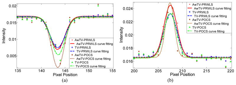
Horizontal profiles of the CatPhan® 600 phantom images reconstructed by different algorithms from 79-view 80mA projection data. Picture (a) shows the profiles across the cold spot (146th row, 135th to 155th column). Picture (b) shows the profiles across the hot spot (and 139th row, 200th to 220th column).
III.A.4.3. FWHM measures
The FWHM values of those fitted profiles are shown in Table III, which are consistent with our conclusion for profile comparison. From Table III, we can observe that for full-views 10mA case, the AwTV-PRWLS method has the smallest value compared to other three methods on both cold and hot spots. In the case of 79-views 80mA projection data, the AwTV-POCS has the smallest value which corresponds to the highest resolution. In the case of 79-views 10mA projection data, all the four methods failed to reconstruct good results.
Table III.
The FWHM values of the cold and hot spots in Fig. 9
| Data type of projection | Position | AwTV-PRWLS | TV-PRWLS | AwTV-POCS | TV-POCS |
|---|---|---|---|---|---|
| Full-views 10mA | cold spot | 4.7470 | 4.7565 | 4.9797 | 4.9816 |
| hot spot | 4.6836 | 4.9891 | 4.8880 | 5.0220 | |
| 79-views 80mA | cold spot | 5.0455 | 5.0689 | 4.8504 | 4.9162 |
| hot spot | 4.4650 | 4.4979 | 2.9963 | 4.2629 | |
| 79-views 10mA | cold spot | 3.9222 | 5.3275 | 3.1866 | 3.6049 |
| hot spot | 5.4802 | 6.1406 | 2.4487 | 4.4086 |
III.B. Anthropomorphic head phantom study
III.B.1. Visualization and profile-based comparison
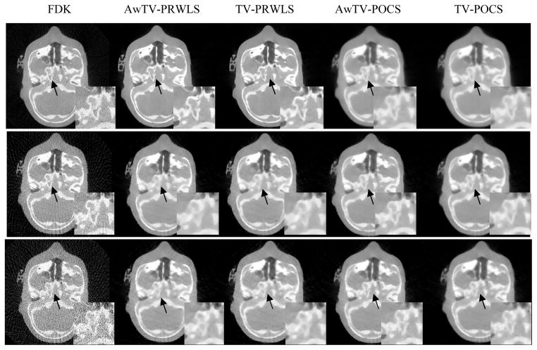
Figure 14 shows the transverse images of the anthropomorphic head phantom reconstructed by different methods from the cone-beam projection data acquired with 125 kVp, 80mA and 10mA protocols. For the cases of sparse-view projection measurements from the 80mA and 10mA, 113 views from the full views were extracted as sparse-view data for image reconstruction.
Fig. 14.
Transverse reconstructed images of the anthropomorphic head phantom. The first row shows the images reconstructed from the full-view 10mA projection data. The second row shows the images reconstructed from the 113-view 80mA projection data. The third row shows the images reconstructed from the 113-view 10mA projection data. The display window is [0, 0.03].
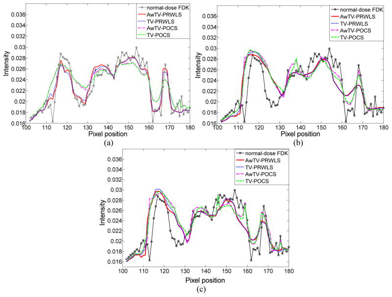
The first column of Fig. 14 shows the images reconstructed by the FDK method from the three types of projection data. It can be observed that the FDK method did not produce satisfactory results from these three types of data due to the noise and artifacts caused by the missing data or both. The first row of Fig. 14 shows the images reconstructed by the FDK, AwTV/TV-PRWLS and AwTV/TV-POCS methods from the full-view 10mA projection data. It can be observed that, in this case, both the AwTV/TV-PRWLS algorithms can efficiently suppress noise without losing the bone structures. On the contrary, to keep the same noise level with the results from AwTV/TV-PRWLS method, the images reconstructed by the AwTV/TV-POCS methods are softer and over-smoothed to suppress noise. The second row of Fig. 14 shows the images reconstructed from the 113-view 80mA projection data. It can be seen that both the AwTV/TV-POCS methods show some advantages compared to the results of the AwTV/TV-PRWLS methods. The third row of Fig. 14 shows the images reconstructed from the 113-view 10mA projection data. It can be seen that all the four strategies mentioned above cannot produce satisfactory results. Furthermore, the associative horizontal profiles across the 102th to 180th columns at the 180th row are plotted in Fig. 15. It can be seen that the profile of the results from AwTV-PRWLS is much closer to the full-view 80mA FDK image in the case of full-views 10mA projection data. In the both the cases of sparse-views with 80mA and 10mA, the AwTV-POCS shows better performance than other methods.
Fig. 15.
The horizontal profiles (102th to 180th columns at 180th row) of the reconstructed images from: (a) the full-view 10mA projection data; (b) the 113-view 80mA projection data; and (c) the 113e-view 10mA projection data.
III.B.2. Resolution-noise tradeoff comparison
Figure 16 shows the curve of the resolution and standard deviation of the background area with different β settings from the full-view 10mA projection data. The resolutions are calculated from the ESF as indicated in Fig. 16(a). It can be observed that in the same background noise level, the results of the AwTV-PRWLS algorithm have higher resolution than the results of the TV-PRWLS algorithm, which is consistent with the results from the CatPhan® 600 phantom study.
Fig. 16.
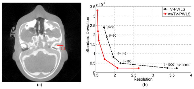
The resolution-noise tradeoff curves: (a) the transverse reconstructed images of the anthropomorphic head phantom; (b) the resolution-noise trade off curves of the TV-PRWLS and AwTV-PRWLS algorithms.
IV. DISCUSSION AND CONCLUSION
In this paper, we presented a statistical image reconstruction method based on the PRWLS strategy for CT image reconstruction. There are two motivations triggered this study. Firstly, we adopted a novel AwTV [12] as a regularization term (i.e., the a priori term) to penalize the RWLS problem, which can mitigate the over-smoothing or recover more edge details compared to the conventional TV penalty. Secondly, the variances of the projection data are estimated with inclusion of the electronic background noise [19], which is considered to accurately describe the statistical property of the low-mAs projection data. Although the effect of the electronic background noise is minor for normal-mAs CT projection data due to the large quantity of photons in the measurement, the detected number of photons in the case of low-mAs scan is dramatically decreased. Thus, the effects of the electronic background noise could not be ignored [19]. In this study, by using a new variance estimation of projection data as weights in the present AwTV-PRWLS strategy, the RWLS term (i.e., the primary term) is more accurate than the uniform WLS without utilizing the statistical property. It should be mentioned that in a penalized likelihood image reconstruction, a widely-used smoothing penalty term can suppress the reconstruction variance dramatically and, therefore, make the task to see the gain by a more accurate variance description even challenging. Nevertheless, despite the challenging, it is not reasonable to reject the use of a more accurate variance description in the penalized likelihood image reconstruction framework.
Through extensive experiments with quantitative and qualitative measures, we found that the AwTV/TV-PRWLS strategies can yield more details than the AwTV/TV-PUWLS strategies in all three types of datasets. For example, as we can see from the resolution-noise tradeoff curves and the FWHM studies, the advantage of the AwTV term compared to the conventional TV term is significant noticeable. Furthermore, the AwTV-based strategies show more efficiency to accurately preserve edge details than the conventional TV term.
In the present study, besides the comparison between the AwTV/TV-PRWLS and AwTV/TV-PUWLS strategies, we also executed a comparison between the AwTV/TV-PRWLS strategies and the well-known AwTV/TV-POCS strategies with three types of datasets. Both the FWHM value and visual comparison via displaying the results of the AwTV/TV-PRWLS and AwTV/TV-POCS strategies have demonstrated that the AwTV/TV-PRWLS methods can reconstruct satisfactory image from full-view 10mA projection data. Compared to the AwTV/TV-PRWLS strategies, the AwTV/TV-POCS strategies require that the estimated projections data should obey high fidelities to the observed projection data. Meanwhile, in practice, this condition is really hard to be met in low-mAs CT measurements. On the other side, the PRWLS model can be mathematically proven to follow the concept of maximum a posteriori (MAP) estimation, which fully utilizes the statistical property of the noise model of the signal. As a result, the AwTV/TV-PRWLS strategies could converge to a close solution when the number of projections is enough. As shown in section III.A.4 and III.B, we can conjecture the AwTV/TV-PRWLS strategies would show some advantages than the AwTV/TV-POCS strategies in full-projection view case. We may conclude that PRWLS method can obtain a more accurate solution the other present method in this study.
In the studies using the sparse-view 80mA projection data, both the AwTV/TV-POCS strategies show more advantages than the AwTV/TV-PRWLS strategies in terms of achieving smaller FWHM values. Due to the piecewise constant hypothesis and the knowledge of the high SNR of the observed data, the AwTV/TV-POCS strategies always aim to find an unique optimal solution having a minimum AwTV/TV value from the feasible region [30]. However, the AwTV/TV-PRWLS strategies always look for the solution from an unconstraint minimization problem, which indicated there would be multiple candidate solutions meet the minimization condition [6]. In addition, there is no such mechanism to tell us which is the best. Thus, it could be more possible to reconstruct a satisfactory result from a sparse-view 80mA case by using the AwTV/TV-POCS strategies.
It is worth to note that all AwTV/TV-POCS and AwTV/TV-PRWLS algorithms fail to produce satisfactory results in the case of the sparse-view 10mA projection data. One possible reason is that there are always some unsatisfied conditions for using these two types of strategies (i.e., the low-fidelity of the detected projection data in the POCS strategy and the low number of observations in the PRWLS strategy).
In summary, the presented AwTV-PRWLS strategy is a more efficient way to accurately reconstruct the image from low-mAs (i.e., 10mA) full projection data and the AwTV-POCS strategy is a more efficient way to reconstruct the image from sparse-view normal-mAs (i.e., 80mA) projection data. As we mentioned at the beginning of this paper, the efficiencies of the AwTV model compared to other priors are still unknown and shall be investigated further. Therefore, the comparison between the AwTV prior and other prior terms, such as the generalized Gaussian Markov random field (GGMRF) prior [31], the reweight TV prior [32], the TV-stokes prior [33] or the prior information from previous scan [13, 34, 35], will be one task in our further research. In addition, how to solve the TV/AwTV problem efficiently and accurately will be another task in our future studies [36, 37]. Another interesting topic is how to utilize TV-based image reconstruction methods toward different clinical applications, such as high resolution micro-CT [38] and multiple objects reconstruction [39], which could be another task in our future work.
Acknowledgments
This work was partially supported by the NIH/NCI under Grant #CA143111 and #CA082402. J. Ma also was partially supported by the NSF of China under Grant #81000613 and #81101046 and the National Key Technologies R&D Program of China under Grant #2011BAI12B03. The authors are grateful to the editing effort from Ms. Donna Carroll.
References
- 1.Brenner D, Hall E. Computed Tomography – An Increasing Source of Radiation Exposure. N ENGL J MED. 2007;357:2277–2284. doi: 10.1056/NEJMra072149. [DOI] [PubMed] [Google Scholar]
- 2.Kalra MK, Wittram C, Maher MM, Sharma A, Avinash GB, Karau K, Halpern TL, Saini S, Shepard JA. Can noise reduction filters improve low-radiation-dose chest CT images? Pilot study. Radiology. 2003;228(1):257–264. doi: 10.1148/radiol.2281020606. [DOI] [PubMed] [Google Scholar]
- 3.Smith A, Dillon W, Gould R, Wintermark M. Radiation dose-reduction strategies for neuroradiology CT protocols. American Journal of Neuroradiology. 2007;28(9):1628–1632. doi: 10.3174/ajnr.A0814. [DOI] [PMC free article] [PubMed] [Google Scholar]
- 4.McCollough CH, Primak AN, Braun N, Kofler J, Yu L, Christner J. Strategies for reducing radiation dose in CT. Radiologic Clinics of North America. 2009;47(1):27–40. doi: 10.1016/j.rcl.2008.10.006. [DOI] [PMC free article] [PubMed] [Google Scholar]
- 5.Sidky E, Kao C, Pan X. Accurate image reconstruction from few-views and limited angle data in divergent-beam CT. Journal of X-Ray Science and Technology. 2006;14(2):119–139. [Google Scholar]
- 6.Sidky E, Pan X. Image reconstruction in circular cone-beam CT by constrained, total-variation minimization. Physics in Medicine and Biology. 2008;53:4777–4807. doi: 10.1088/0031-9155/53/17/021. [DOI] [PMC free article] [PubMed] [Google Scholar]
- 7.Li T, Li X, Wang J, Wen J, Lu H, Hsieh J, Liang Z. Nonlinear sinogram smoothing for low-dose X-ray CT. IEEE Transactions on Nuclear Science. 2004;51:2505–2513. [Google Scholar]
- 8.Wang J, Li T, Lu H, Liang Z. Penalized weighted least-squares approach to sinogram noise reduction and image reconstruction for low-dose X-ray CT. IEEE Transactions on Medical Imaging. 2006;25(10):1272–1283. doi: 10.1109/42.896783. [DOI] [PMC free article] [PubMed] [Google Scholar]
- 9.La Rivière PJ, Bian J, Vargas PA. Penalized-likelihood sinogram restoration for CT. IEEE Transactions on Medical Imaging. 2006;25(8):1022–1036. doi: 10.1109/tmi.2006.875429. [DOI] [PubMed] [Google Scholar]
- 10.Bian J, Siewerdsen Jh, Han X, Sidky EY, Prince JL, Pelizzari CA, Pan X. Evaluation of sparse-view reconstruction from flat-panel-detector cone-beam CT. Physics in Medicine and Biology. 2010;55:6575–6599. doi: 10.1088/0031-9155/55/22/001. [DOI] [PMC free article] [PubMed] [Google Scholar]
- 11.Donoho D. Compressed sensing. IEEE Transactions on Information Theory. 2006;52(4):1289–1306. [Google Scholar]
- 12.Liu Y, Ma J, Fan Y, Liang Z. Adaptive-weighted total variation minimization for sparse data toward low-dose x-ray computed tomography image reconstruction. Physics in Medicine and Biology. 2012;57:7923–7956. doi: 10.1088/0031-9155/57/23/7923. [DOI] [PMC free article] [PubMed] [Google Scholar]
- 13.Chen G, Tang J, Leng S. Prior image constrained compressed sensing (PICCS) Proc Soc Photon Instrum Eng. 2008;6856:1–18. doi: 10.1117/12.770532. [DOI] [PMC free article] [PubMed] [Google Scholar]
- 14.Hsieh J. Adaptive streak artifact reduction in CT resulting from excessive X-ray photon noise. Med Phys. 1998;25:2139–2147. doi: 10.1118/1.598410. [DOI] [PubMed] [Google Scholar]
- 15.Xu J, Tsui BM. Electronic noise modeling in statistical iterative reconstruction. IEEE Transactions on Medical Imaging. 2009;18(6):1228–1239. doi: 10.1109/TIP.2009.2017139. [DOI] [PMC free article] [PubMed] [Google Scholar]
- 16.Elbakri IA, Fessler JA. Statistical image reconstruction for polyenergetic X-ray CT. IEEE Transaction on Medical Imaging. 2002;21(2):89–99. doi: 10.1109/42.993128. [DOI] [PubMed] [Google Scholar]
- 17.Elbakri IA, Fessler JA. Efficient and accurate likelihood for iterative image reconstruction in X-ray CT. Proceeding of SPIE Medical Imaging 2003. 2003;5032:1839–1850. [Google Scholar]
- 18.Wang J, Li T, Xing L. Iterative image reconstruction for CBCT using edge-preserving prior. Medical Physics. 2009;36(1):252–260. doi: 10.1118/1.3036112. [DOI] [PMC free article] [PubMed] [Google Scholar]
- 19.Ma J, Liang Z, Fan Y, Liu Y, Huang J, Chen W, Lu H. Variance abalysis of x-ray CT sonograms in the presence of electronic noise background. Medical Physics. 2012;39(7):4051–4065. doi: 10.1118/1.4722751. [DOI] [PMC free article] [PubMed] [Google Scholar]
- 20.Yu H, Wang G. A soft-threshold filtering approach for reconstruction from a limited number of projections. Physics in Medicine and Biology. 2010;55:3905–3916. doi: 10.1088/0031-9155/55/13/022. [DOI] [PMC free article] [PubMed] [Google Scholar]
- 21.Defrise M, Vanhove C, Liu X. An algorithm for total variation regularization in high-dimensional linear problems. Inverse Problem. 2011;6:065002. [Google Scholar]
- 22.Ouyang L, Timothy S, Wang J. Effects of the penalty on the penalized weighted least-squares image reconstruction for low-dose CBCT. Physics in Medicine and Biology. 2011;56:5535–5552. doi: 10.1088/0031-9155/56/17/006. [DOI] [PubMed] [Google Scholar]
- 23.Ramni S, Fessler J. Convergent Iterative CT Reconstruction Sparsity-Based Regularization. Fully3D conference proceeding. 2011:302–305. [Google Scholar]
- 24.Yan M, Vese HLA. Expectation Maximization and Total Variation Based Model for Computed Tomography Reconstruction form Undersampled Data. Proceedings of SPIE Medical Imaging 2011. 2011:7961. [Google Scholar]
- 25.Whiting BR. Signal statistics of X-ray CT. Proceedings of SPIE Medical Imaging 2002. 2002:4682. [Google Scholar]
- 26.Lasio GM, Whiting BR, Williamson JF. Statistical reconstruction for X-ray CT using energy-integration detectors. Physics in Medicine and Biology. 2007;52:2247–2266. doi: 10.1088/0031-9155/52/8/014. [DOI] [PubMed] [Google Scholar]
- 27.Ma J, Feng Q, Feng Y, Huang J, Chen W. Generalized Gibbs priors based positron emission tomography reconstruction. Computers in Biology and Medicine. 2010;40(6):565–571. doi: 10.1016/j.compbiomed.2010.03.012. [DOI] [PubMed] [Google Scholar]
- 28.Fessler JA. Penalized weighted least-squares image reconstruction for Positron emission tomography. IEEE Transactions on Medical Imaging. 1994;13(2):290–300. doi: 10.1109/42.293921. [DOI] [PubMed] [Google Scholar]
- 29.Wang J, Li T, Liang Z, Xing L. Dose reduction for kilovotage cone-beam computed tomography in radiation therapy. Physics in Medicine and Biology. 2008;53:2897–2909. doi: 10.1088/0031-9155/53/11/009. [DOI] [PubMed] [Google Scholar]
- 30.Candès E, Romberg J, Tao T. Robust uncertainty principles: Exact signal reconstruction from highly incomplete frequency information. IEEE Transactions on Information Theory. 2006;52(2):489–509. [Google Scholar]
- 31.Bouman C, Sauer K. A Generalized Gaussian Image Model for Edge-Preserving MAP Estimation. IEEE Transactions on Medical Imaging. 1993;2(3):296–310. doi: 10.1109/83.236536. [DOI] [PubMed] [Google Scholar]
- 32.Chang M, Li L, Chen Z, Xiao Y, Zhang L, Wang G. A few-view reweighted sparsity hunting (FRESH) method for CT image reconstruction. Journal of X-Ray Science and Technology. 2013;21(2):161–176. doi: 10.3233/XST-130370. [DOI] [PubMed] [Google Scholar]
- 33.Liu Y, Liang Z, Ma J, Lu H, Wang K, Zhang H, Moore W. Total Variation-Stokes Strategy for Sparse-View X-ray CT Image Reconstruction. IEEE Transactions on Medical Imaging. 2014;33(3):749–763. doi: 10.1109/TMI.2013.2295738. [DOI] [PMC free article] [PubMed] [Google Scholar]
- 34.Ma J, Huang J, Zhang H, Feng Q, Lu H, Liang Z, Chen W. Low-Dose Computed Tomography Image Restoration Using Previous Normal-Dose Scan. Medical Physics. 2011;38(10):5713–5731. doi: 10.1118/1.3638125. [DOI] [PMC free article] [PubMed] [Google Scholar]
- 35.Ma J, Zhang H, Gao Y, Huang J, Liang Z, Feng Q, Chen W. Iterative Image Reconstruction for Cerebral Perfusion CT Using a Pre-contrast Scan Induced Edge-Preserving Prior. Physics in Medicine and Biology. 2012;57:7519–7542. doi: 10.1088/0031-9155/57/22/7519. [DOI] [PMC free article] [PubMed] [Google Scholar]
- 36.Jian X, Lou Y, Lewis J, Li R, Gu X, Men C, Song WY, Jiang SB. GPU-based fast low-dose cone beam CT reconstruction via total variation. Journal of X-ray Science and Technology. 2011;19(2):139–154. doi: 10.3233/XST-2011-0283. [DOI] [PubMed] [Google Scholar]
- 37.Khaled AS, Beck TJ. Successive binary algebraic reconstruction technique: An algorithm for reconstruction from limited angle and limited number of projections decomposed into individual components. Journal of X-ray Science and Technology. 2013;21(1):9–24. doi: 10.3233/XST-130363. [DOI] [PubMed] [Google Scholar]
- 38.Sen Sharma K, Jin X, Holzner C, Narayanan S, Liu B, Wang D, Agah M, Wang L, Yu H, Wang G. Experimental studies on few-view reconstruction for high-resolution micro-CT. Journal of X-ray Science and Technology. 2013;21(1):25–42. doi: 10.3233/XST-130364. [DOI] [PubMed] [Google Scholar]
- 39.Lu Y, Tang Z, Zhao J, Wang G. TV-based image reconstruction of multiple objects in a fixed source-detector geometry. Journal of X-Ray Science and Technology. 2012;20(3):277–289. doi: 10.3233/XST-2012-0337. [DOI] [PubMed] [Google Scholar]


