A practical introduction to skeletons for the plant sciences

Abstract

Before the availability of digital photography resulting from the invention of charged couple devices in 1969, the measurement of plant architecture was a manual process either on the plant itself or on traditional photographs. The introduction of cheap digital imaging devices for the consumer market enabled the wide use of digital images to capture the shape of plant networks such as roots, tree crowns, or leaf venation. Plant networks contain geometric traits that can establish links to genetic or physiological characteristics, support plant breeding efforts, drive evolutionary studies, or serve as input to plant growth simulations. Typically, traits are encoded in shape descriptors that are computed from imaging data. Skeletons are one class of shape descriptors that are used to describe the hierarchies and extent of branching and looping plant networks. While the mathematical understanding of skeletons is well developed, their application within the plant sciences remains challenging because the quality of the measurement depends partly on the interpretation of the skeleton. This article is meant to bridge the skeletonization literature in the plant sciences and related technical fields by discussing best practices for deriving diameters and approximating branching hierarchies in a plant network.

The advent of digital imaging accelerated the development of computational methods to digitally reconstruct the shape of plant networks from imaging data. From reconstructions, detailed measurements such as network width or diameters of network links can be derived for a plant network. The importance of reconstructions and measurements (Godin, 2000; Spalding and Miller, 2013) is founded in the many known or hypothesized links between plant network properties and actual functions of plants (Brodribb and Feild, 2000; Enquist, 2002; Lynch, 2011; Lynch and Brown, 2012). In particular, roots system architecture (Lynch, 1995; de Dorlodot et al., 2007), tree crown architecture (Delagrange et al., 2004), or leaf vein structures (Roth-Nebelsick et al., 2001; Mason et al., 2013; Price et al., 2013) are examples of plant networks. Measurements of such networks are analyzed in the context of genotype to phenotype mapping (El-Soda et al., 2014) as well as breeding efforts (Holland et al., 2003; Finkel, 2009), evolutionary studies of plant species (Green and Hickey, 2005; Fernandez et al., 2010; Feild et al., 2011), or plant growth simulation (Vansteenkiste et al., 2014).

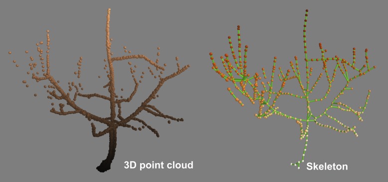
Images encode the shape of plant networks such as roots, tree crowns, or leaf venation. Most commonly, images are digitally represented in a two- or three-dimensional raster of pixels or of voxels, respectively. Some imaging techniques produce point clouds of 3D coordinates that often employ no neighborhood information between the points. Recently, the combination of imaging data with skeletonization algorithms became popular as a tool to extract the hierarchies and geometric measurements of plant networks. Skeletons consist of a collection of (approximated) curves being mostly centered within the plant network of interest (Fig. 1). In this article, I discuss the fundamental characteristics of imaging data in the context of studying plant networks and give an overview of existing skeletonization concepts. Within the skeletonization overview, I highlight concepts that were applied to plant networks. In the remainder of the article, I introduce two basic skeleton concepts in detail and demonstrate their applicability to plant networks on selected examples.

Fig. 1.

3D point cloud data obtained with a terrestrial laser scanner and the corresponding curve approximation skeleton of an orchard tree. The skeleton was computed with SkelTre (Bucksch et al., 2010).

THE BOUNDARY CONCEPT AND OCCLUSION IN IMAGING DATA

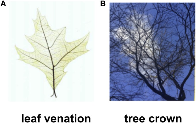
Before applying skeletonization algorithms, it is important to understand the intrinsic constraints of imaging data. Imaging technologies capture data about an object surface and/or interior within the specification of an imaging sensor. For example, a digital photo camera collects the light reflected from surfaces that face the photo sensor. At each location of the photo sensor, a value for the received wavelength is stored as an electrical potential or as the number of photons counted within a certain time frame. The stored wavelength corresponds to colors that we recognize in the pixels of the image. In the case of a plant network, this physical process of capturing light is a projection of the plant network onto a plane. The result is a 2D image that encodes the form of a plant network. For leaf venation networks, this projection does not cause any self-occlusion (Fig. 2). However, the projection onto the 2D plane comes at a cost for other plant networks such as heavily branched tree crowns or dense roots. In both cases, branches will occlude parts of the tree crown (Fig. 2) or rootstock. As a result, the digital photograph misses network information at all self-occluded locations. Similar to recording reflections of light, it is also possible to record absorption rates of wavelengths that penetrate the plant network.

Fig. 2.

Plant networks with and without occlusion. (A) Image of a cleared leaf with its venation network visible. The venation network is not occluding itself through the projection onto the image plane. Image taken from http://clearedleavesdb.org (Das et al., 2014). (B) Image of a tree crown. The branches occlude each other, such that the image does not contain the information of the complete branches.

3D imaging technologies improve upon the occlusion problem. In general, 3D data are obtained from the reflection of waves from the plant surface or from waves penetrating the plant network such that the absorption rate varies through different tissues. Technologies relying on the reflection of light from a surface include structured light methods that project a known pattern onto the plant network and calculate 3D information from the distortion of the projected pattern (Salvi et al., 2004). Another technology is terrestrial laser scanning (Vosselman and Maas, 2010) that relies on the reflection of laser beams from the surfaces. The round-trip time of the laser from the sensor to surface determines the distance between sensor and surface because of the constant speed of light. In practice, occlusion effects still occur as missing data, but can be minimized by using registration techniques to combine different views of the plant network (Bucksch and Koshelham, 2013). The benefit of the obtained 3D information is that distribution of the network in 3D space allows the use of prior knowledge, such as assuming allometric relations in a branching structure (Aiteanu and Klein, 2014), to recover an approximation of the network. Ideally, the occlusion problem is resolvable with imaging technologies that penetrate the plant network, such as X-ray (Mairhofer et al., 2013) or magnetic resonance imaging (Schulz et al., 2013), that record changing absorption rates in different plant tissues. As a result, not only the outer surface, but also the internal architecture of the plant is resolvable. The important commonality between all these imaging technologies is that the plant network is represented as a boundary between itself and the free space surrounding the object in 2D and 3D. Or, more intuitively spoken, the boundary of a 3D plant network separates its enclosed volume from its “outside” environment. Data representations that just encode the plant network and the “outside” are called binary, because they assign a 1 to every plant network location and a 0 to every background location. In most application scenarios, we can safely assume the boundary of a plant network to be smooth, i.e., the boundary has no sharp corners or breaklines.

Once we understand the concept of a boundary, we can observe that skeletons are derived from this interface between the plant network and environment. Thus, a skeleton representation is computed on the basis of the boundary and, therefore, a skeleton represents boundary properties rather than the hierarchies and extensions of biological interest.

SKELETON CONCEPTS AND PLANT APPLICATIONS

Current literature reviews a plethora of skeleton concepts to be computed from 2D binary images (Lam et al., 1992), 3D images of voxels (Sobiecki et al., 2014), and point clouds (Cornea and Min, 2007; Bucksch, 2011). Two basic skeleton concepts used today are the medial axis (Lee, 1982) and the Reeb graph (Biasotti et al., 2008) shown in Fig. 3. The computation of the medial axis can be performed on 2D binary images (Serra, 1986), 3D voxels (Palágyi, 2002), and point clouds (Amenta et al., 2001). A noteworthy extension is the Hamilton-Jacobi skeleton (Siddiqi et al., 2002), which enhances the medial axis with a flux equation to achieve more robustness to noise. In recent years, the field of computer graphics developed several new skeleton concepts that make use of prior knowledge of the plant network. Rotational symmetry axis (ROSA) assumes rotational symmetry around the skeletal curves to enhance robustness against missing data from point clouds (Tagliasacchi et al., 2009). The assumption of a tree structure to extract a skeleton from point cloud data was introduced in Livny et al. (2010) for trees and has been applied to plant networks of grape clusters (Schöler and Steinhage, 2012; Steinhage et al., 2012). A very recent concept is the L₁-medial skeleton (Huang et al., 2013), which shows promising results on point clouds of plants.

Fig. 3.

Comparison of the medial axis and the Reeb graph for a simple rectangle. The medial axis (MA) was extracted using a morphological thinning algorithm. Examples are shown of corresponding circles whose center (c) build the medial axis and touch the boundary of the plant network M in two points. The Reeb graph (RG) was computed using the height function F to extract the contours (green line) at height levels i₁ and i₂ from the rectangular plant network M at intervals of s. The center of the contracted contour is marked with a cross. The source code for all examples is available on https://github.com/abucksch.

The use of skeletonization algorithms to obtain quantitative measurements of plant networks was first applied on tree crowns to estimate the radiative properties by simulating the foliage and fine branches from laser data (Cote et al., 2009) and to derive branch hierarchy information along with length and diameter distributions (Bucksch and Fleck, 2011; Delagrange et al., 2014). Leaf veins were quantified with skeletons to obtain estimates of areole measures and hierarchies (Price et al., 2011, 2013, 2014; Price, 2012). A recent article introduced a framework to identify legumes on the basis of leaf vein features (Larese et al., 2014). The branching structure of roots is another plant network that is often assessed with skeletons to obtain measurements of phenotypic traits (Iyer-Pascuzzi et al., 2010; Clark et al., 2011; Galkovskyi et al., 2012; Pound et al., 2013) to be related to regions of the genome (Topp et al., 2013). Pound et al. (2013) introduced a skeletonization concept for plant phenotyping that uses a probability field computed from the gray values of a 2D image to grow a connected skeleton of young and sparse roots. The growth is initiated at a user-defined location to the root tips. Free software exists that allows manual enforcement of skeleton centeredness and correction of miscomputed branching hierarchy. The references for tree crowns are examples of successful applications developed on the basis of a Reeb graph. Except for Pound et al. (2013), the chosen examples for leaves and roots apply to the medial axis.

Medial axis

The medial axis (Fig. 3) was introduced by Harry Blum (Blum, 1967) and was inspired by line-like structures created by the process of extinguishing fires. Simply imagine a patch of dry grassland, the whole border of which is ignited at one moment in time. If the fire propagates inward at a constant speed, then the fire fronts meet at the location of the medial axis. Although there is no generally agreed-upon definition of the medial axis (Attali et al., 2009), we can use here a simplified definition that can be visually followed in Fig. 3 using the same variables. The medial axis MA of a plant network M with a smooth boundary is the set of points inside the root network that consists of centers (c_i) of circles in two dimensions or spheres in three dimensions, whose boundary touches in at least two points (t_i,_j and t_i,_j+1) the boundary of the plant network. Here, touching is used as a synonym for the circle/sphere being tangent to the boundary of M.

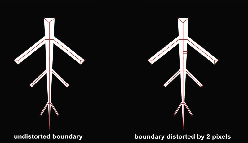
The definition of the medial axis implies that each local change of the boundary changes the medial axis. Such changes correspond to locally occurring/vanishing maxima, minima, or saddle points on the boundary. Consequently, additional branches occur in the medial axis that may not represent the actual network. Reasons for additional branches include noise in the imaging data and tissue growth that results in a locally bulging boundary (Fig. 4). As a result, direct biological interpretation from the medial axis skeleton is problematic. A simple but efficient correction that makes use of a property of the medial axis is to remove branches that are shorter than the known radius of a circle/sphere at a branching point plus a user-defined threshold. In some applications, a threshold might be hard to define, such that methods to prune the medial axis have to be applied (e.g., Bai et al., 2007).

Fig. 4.

Sensitivity of the medial axis to boundary distortions. Two pixels were added to the boundary, which results in two extra branches that do not belong to the plant network hierarchy.

One problem arising in 3D applications of the medial axis is the occurrence of planes. For many plant applications, this problem is irrelevant, because plant organs are often cylindrical or planar and therefore result in curves. However, there are solutions to reduce these planes to curves (Palágyi and Kuba, 1998; Gorte and Pfeifer, 2004).

Reeb graph

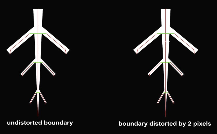
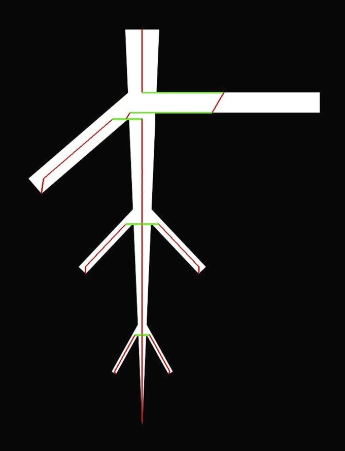
The Reeb graph (Fig. 3) is a skeletonization concept introduced in 1946 (Reeb, 1946) and used to describe the change of an object shape in relation to a function expanded over the object. A simple way to imagine a Reeb graph is to think of a banana sliced—lengthwise—by a knife. The path of the knife along the banana can be thought of as the function that is expanded over the banana. The centers of the cutting area through the banana are the points on the Reeb graph that get connected to the center of the next cutting area in direction of the path. The following formal definition can be graphically followed in Fig. 3. Given a plant network M with smooth boundary and a piecewise linear function F, the level set at a value i is defined as the set of points in M with function value equal to i. As a practical example, if F is the height function whose function values are the values along the y-axis of a Cartesian coordinate system, then the level sets are simply the intersections when slicing through the object at intervals of size s orthogonal to the y-axis. To obtain the Reeb graph, we analyze the change of the connected components of the level sets of F, called contours. The Reeb graph RG of F is obtained by contracting the contours of F to points. For plants, this point can be chosen as the center of the contour, because most contours are convex. The center points of the contours assemble the vertices of the Reeb graph, which are connected via edges to the “closest” vertices obtained at the next function value i+s. For easier understanding, the given definition includes the embedding of the graph into the plant network. The original literature on Reeb graphs uses an abstract definition, which only defines the merge and split of contours free of coordinates. An example of the introduced construction is shown in Fig. 5 with the same binary images used in Fig. 4. Additionally, Fig. 5 demonstrates the robustness of the Reeb graph to small changes on the boundary.

Fig. 5.

Reeb graph of a simple branching structure extracted with the height function. Vertices are marked in red. Edges are marked in green if the distance between two vertices is larger than two pixels. At these center points, diameter measurements can be derived without interpolation of a curve between two vertices. The level sets were extracted at intervals of one pixel. The robustness of the Reeb graph to small disturbances of the boundary is demonstrated in the example in Fig. 3.

The contours obtained by using height function are horizontal slices through the plant network. Problems can arise because the height function is not rotation invariant. To understand the potential problems, consider the Reeb graph of a vertical trunk of a plant network with a child branch emerging at a 90° angle from a parent branch (Fig. 6). At the level of the child branch, the contours include both the child and parent branch. Hence, only one contour for parent and child branch is extracted. As a result, consecutive center points appear to be “far from each other” or “shifted.”

Fig. 6.

Problems arising from the choice of the contour-extracting function F. The height function is not rotation invariant, which results in a local shift of the Reeb graph at the location where a branch is emerging at a 90° angle.

A different choice of the function F can result in different Reeb graphs that can overcome the problems of the height function. Several solutions have been suggested to choose a suitable function F. Known solutions include the choice of different global functions (Biasotti et al., 2000) or determining a suited function locally (Biasotti et al., 2008; Bucksch et al., 2010), as shown in Fig. 7.

Fig. 7.

Solution to rotation invariance. (A) A point cloud of a tree obtained with a terrestrial laser scanner. (B) A computed SkelTre skeleton that contains the Reeb graph. The computation changes locally the function to extract the contours. (C) The extracted contours of the tree on the left colored randomly. The highlighted red boxes show a noncentered skeleton part and the extracted contours. Image taken from Bucksch et al. (2010). With permission from Springer Science+Business Media: Visual Computer, SkelTre: Robust skeleton extraction from imperfect point clouds, Vol. 26, 2010, pp. 1283–1300, A. Bucksch, R. Lindenbergh, and M. Menenti, Fig. 5.

APPROXIMATING THE BRANCHING HIERARCHY OF A PLANT FROM REAL DATA

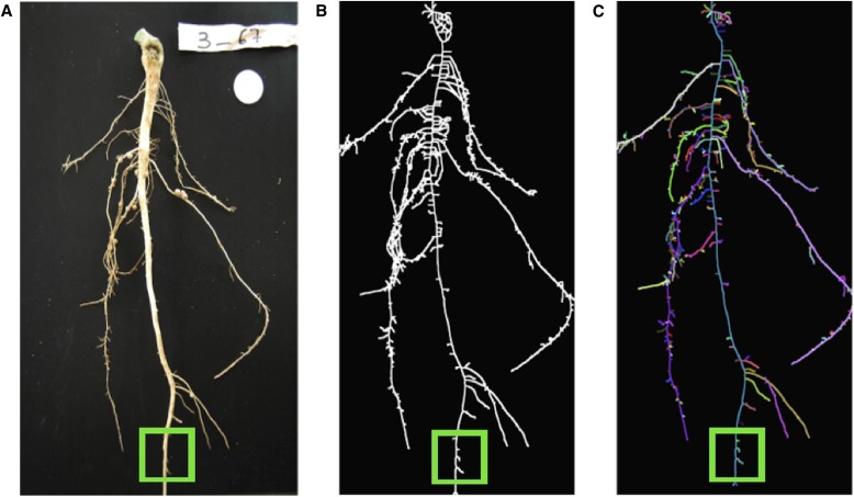
In Fig. 8, the medial axis and its segmentation of a cowpea root system was computed from a 2D image. The segmentation allows the detection of branches that do not represent the actual plant architecture. The segmentation was achieved by tracing the shortest path from the tip of the medial axis closest to the top row of the image to every root tip that is represented in the medial axis. The tracing resolves approximately for the loops resulting from the projection of the three-dimensional arrangement of roots to the image plane. Note that this strategy only applies to sparse networks, where branches do not occlude each other.

Fig. 8.

Detecting medial axis parts for removal. (A) A digital image of a cowpea root. (B) The medial axis derived from the image. (C) The segmented skeleton with random colors for each detected branch. Smaller branches are now removable by using a threshold and the known radius of the medial circle at the tip of each branch. The green box indicates an example area where additional branches can be removed.

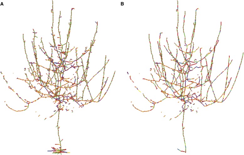
Figure 9 shows a 3D skeleton of a tree crown. Here, the skeleton is represented as a graph embedded into the original point cloud of a tree. All vertices with one incident edge that connect to vertices with three or more incident edges are removed from the originally extracted graph. The resulting skeleton approximates the actual branching structure of the tree crown (Bucksch, 2011).

Fig. 9.

(A) Removal of additional branches with the SkelTre skeleton graph. (B) Vertices with only one incident edge and an adjacent vertex with three or more incident edges removed. Image taken from Bucksch (2011).

SKELETON CENTEREDNESS USED TO DERIVE DIAMETERS IN PLANT APPLICATIONS

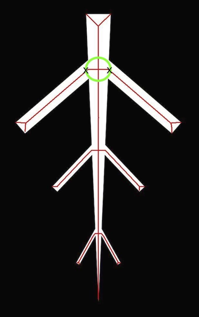
For plant networks, noncentered skeleton parts occur at locations where a child branch emerges from a parent branch (Fig. 7 and Fig. 10). Noncenteredness is implicit because a skeleton is a one-dimensional representation of a plant network that expands in two or three dimensions. This expansion is what we visually recognize as thickness and can be seen as the result of the expansion process of a growing one-dimensional curve (Bucksch et al., 2014). Therefore, every connected skeleton of a branching plant network travels from a branching point through a region of “thickness” before it reaches the location where the branch emerges from the boundary (Fig. 10). As a result, the skeleton part between the branching point and the point of branch emergence on the boundary is not centered. In the case of the medial axis, we can simply subtract the radius of the medial circle at the branching point from the emerging skeletal branch. In the case of the Reeb graph, we may identify jumps in the size of the contour on suited data. As a result, we obtain an approximation of the point of branch emergence on the boundary. Computing the point of branch emergence corresponds closely to measurements that can be obtained manually on the real plant, e.g., with a measuring tape, when measuring along the surface of the branch from the start of a branch on the trunk surface to the tip. For the Reeb graph, we can detect such regions as “long edges.” Note that vertices are favorable locations to derive measurements from the plant network because the graph can maintain centeredness for its vertices while the edges are not necessarily centered.

Fig. 10.

Noncentered locations of the medial axis within the green medial circle. To be a connected skeleton, the medial axis passes through an area of the object interior before reaching the point of branch emergence marked with a cross.

A QUANTITATIVE EXAMPLE OF SKELETON-DRIVEN TRAIT COMPUTATION

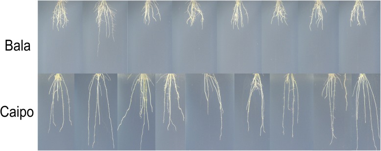
In the following, I apply the introduced skeleton concepts to images from a freely available rice root data set used in Iyer-Pascuzzi et al. (2010). The data set consists of images that show the root from several side views. I selected one image per individual root of the Caipo and Bala genotypes. Each image was selected such that occlusion of roots is visually minimized, which corresponds to the view of maximal root width. Overall, I used nine images of the Caipo data set and eight images of the Bala data, shown in Fig. 11. Both data sets were imaged with the same imaging setup such that results measured in pixels are comparable. The origin of the image is set to be the upper left corner. The absolute value of the negative y-direction corresponds to the row numbers.

Fig. 11.

The Bala and Caipo images. Maximum tip diameter, root width, and rooting depth were extracted to differentiate both genotypes from each other.

The three example traits—maximum tip diameter, root width, and rooting depth—were computed for the selected Bala and Caipo images. Caipo and Bala were chosen because they visually contrast with each other in these traits (Fig. 11). A tip on the medial axis is defined as a pixel with only one neighbor and the diameter is known from the corresponding medial circle. To estimate root width, I used the difference between maximal and minimal column values occupied by the skeleton. Rooting depth corresponds to the maximal row number reached by one of the tips. I also applied noise filtering with a threshold of two pixels to eliminate branches resulting from noise as described above.

Caipo shows a maximum tip diameter of 3.9 pixels with a standard deviation (SD) of 0.57. Bala resulted in a maximum tip diameter of 4.4 pixels (SD = 0.50). A t-test performed on the two measurement sets resulted in a P = 0.13 and suggests that the maximum tip diameter differentiates both genotypes. Furthermore, I extracted estimates of the two known traits—root width and rooting depth. Root width resulted in an average of 607.11 pixels (SD = 224.90) for Caipo and an average of 504.38 pixels (SD = 66.14) for Bala. Although the t-test resulted only in P = 0.23 for the small set of test images, the genotypes differed strongly in their standard deviation. The strongest differentiation (P < 0.0001) between the two genotypes was achieved with the rooting depth. Rooting depth of Caipo was 1317.80 pixels (SD = 151.35) on average. In comparison, the rooting depth of Bala was about half as deep as the rooting depth of Caipo, resulting in an average of 625.50 pixels (SD = 181.62). I used an early version of the Digital Imaging of Root Traits (DIRT) platform (www.dirt.biology.gatech.edu) to compute the traits from the medial axis. The computation results are included in Appendix S1 ^{(29KB, xls)} .

DISCUSSION

The advancement of image processing algorithms has resulted in a wide variety of software tools throughout biology (Eliceiri et al., 2012) and the plant sciences in particular (Lobet et al., 2013). In addition to end-user software, open-source libraries for scripting languages such as MATLAB or Python (Coelho, 2013; van der Walt et al., 2014) offer access to skeletonization methods. In particular, Python and its scientific libraries have become widely used in interdisciplinary research and education (Deutsch, 2014). Software libraries enable researchers to adapt skeletonization methods to their specific applications. Specific application needs can often be solved via open community platforms such as MATLAB Central, stack overflow, or stack exchange that offer access to source code for easy tasks, such as implementations of 3D skeletonizations in MATLAB (Schena, 2004) or finding branches in a skeleton (stackoverflow.com, 2013). From a user perspective, I introduced two skeletonization basic concepts and provided insight into mechanisms that potentially influence the statistical analysis of data computed with available software packages or code snippets collected on the Internet. However, it remains the responsibility of the researcher to judge and document if measurement errors induced by imperfect data or the skeletonization concept have significant influence on the achieved results.

CONCLUSIONS

Skeletons are powerful descriptors for analyzing plant networks, if applied with care. In this article I pointed out two difficulties:

• 1. Spurious branches have to be removed from an extracted skeletal structure to obtain an improved approximation of the actual plant network.

• 2. Diameter measurements of the plant network of interest cannot be derived at all locations of the skeleton.

The choice for a particular skeletonization concept is dependent on the application, but knowledge of the basic underlying concepts will make it easier to adapt source code to plant applications. These adaptions result in improved data quality computed from skeletons. As a consequence of improved data quality, the statistical analysis of the naturally large geometric variations within plant networks is facilitated.

Achieving a one-to-one correspondence between the actual plant network and a skeleton extracted from imaging data are only possible on sparse plant networks. The limiting factor is not the skeleton concept, but the imaging technology and its ability to resolve the complete plant network. Therefore, preparing near-ideal input data will involve manual work to correct for the physical limits imposed by certain imaging technologies. The simple examples shown here should help end-users to judge the results computed with the chosen software or encourage users to contact the author of the software to interpret the results correctly.

Although I used several thresholds in this article, I do not propose them as an optimal algorithmic solution, but as a simple tool to start experiencing and understanding skeleton concepts. Appendix S2 ^{(28KB, docx)} contains annotated references to freely available data, source/pseudo codes, and executable software referenced in this article.

LITERATURE CITED

- Aiteanu F., Klein R. 2014. Hybrid tree reconstruction from inhomogeneous point clouds. Visual Computer 30: 763–771 [Google Scholar]
- Amenta N., Choi S., Kolluri R. K. 2001. The power crust, unions of balls, and the medial axis transform. Computational Geometry 19: 127–153 [Google Scholar]
- Attali D., Boissonnat J.-D., Edelsbrunner H. 2009. Stability and computation of medial axes: A state-of-the-art report. In T. Möller, B. Hamann, and R. D. Russell [eds.], Mathematical foundations of scientific visualization, computer graphics, and massive data exploration, 109–125. Springer, New York, USA. [Google Scholar]
- Bai X., Latecki L. J., Liu W.-Y. 2007. Skeleton pruning by contour partitioning with discrete curve evolution. IEEE Transactions on Pattern Analysis and Machine Intelligence 29: 449–462 [DOI] [PubMed] [Google Scholar]
- Biasotti S., Falcidieno B., Spagnuolo M. 2000. Extended Reeb graphs for surface understanding and description. In G. Bertrand, M. Couprie, and L. Perroton [eds.], Discrete geometry for computer imagery, 185–197. Springer, Berlin, Germany. [Google Scholar]
- Biasotti S., Giorgi D., Spagnuolo M., Falcidieno B. 2008. Reeb graphs for shape analysis and applications. Theoretical Computer Science 392: 5–22 [Google Scholar]
- Blum H. 1967. A transformation for extracting new descriptors of shape. In W. Wathen-Dunn [ed.], Models for the perception of speech and visual form: Proceedings of a symposium, 362–380. MIT Press, Cambridge, Massachusetts, USA.
- Brodribb T., Feild T. 2000. Stem hydraulic supply is linked to leaf photosynthetic capacity: Evidence from New Caledonian and Tasmanian rainforests. Plant, Cell & Environment 23: 1381–1388 [Google Scholar]
- Bucksch A. 2011. Revealing the skeleton from imperfect point clouds. Dr. Hut, Munich, Germany [Google Scholar]
- Bucksch A., Fleck S. 2011. Automated detection of branch dimensions in woody skeletons of fruit tree canopies. Photogrammetric Engineering and Remote Sensing 77: 229–240 [Google Scholar]
- Bucksch A., Koshelham K. 2013. Localized registration of point clouds of botanic trees. IEEE Geoscience and Remote Sensing Letters 10: 631–635 [Google Scholar]
- Bucksch A., Lindenbergh R., Menenti M. 2010. SkelTre: Robust skeleton extraction from imperfect point clouds. Visual Computer 26: 1283–1300 [Google Scholar]
- Bucksch A., Turk G., Weitz J. S. 2014. The fiber walk: A model of tip-driven growth with lateral expansion. PLoS ONE 9: e85585. [DOI] [PMC free article] [PubMed] [Google Scholar]
- Clark R. T., MacCurdy R. B., Jung J. K., Shaff J. E., McCouch S. R., Aneshansley D. J., Kochian L. V. 2011. Three-dimensional root phenotyping with a novel imaging and software platform. Plant Physiology 156: 455–465 [DOI] [PMC free article] [PubMed] [Google Scholar]
- Coelho L. P. 2013. Mahotas: Open source software for scriptable computer vision. Journal of Open Research Software 1: e3 [Google Scholar]
- Cornea N. D., Min P. 2007. Curve-skeleton properties, applications, and algorithms. IEEE Transactions on Visualization and Computer Graphics 13: 530–548 [DOI] [PubMed] [Google Scholar]
- Cote J.-F., Widlowski J.-L., Fournier R. A., Verstraete M. M. 2009. The structural and radiative consistency of three-dimensional tree reconstructions from terrestrial LiDAR. Remote Sensing of Environment 113: 1067–1081 [Google Scholar]
- Das A., Bucksch A., Price C. A., Weitz J. S. 2014. ClearedLeavesDB: An online database of cleared plant leaf images. Plant Methods 10: 8. [DOI] [PMC free article] [PubMed] [Google Scholar]
- de Dorlodot S., Forster B., Pagès L., Price A., Tuberosa R., Draye X. 2007. Root system architecture: Opportunities and constraints for genetic improvement of crops. Trends in Plant Science 12: 474–481 [DOI] [PubMed] [Google Scholar]
- Delagrange S., Jauvin C., Rochon P. 2014. PypeTree: A tool for reconstructing tree perennial tissues from point clouds. Sensors (Basel, Switzerland) 14: 4271–4289 [DOI] [PMC free article] [PubMed] [Google Scholar]
- Delagrange S., Messier C., Lechowicz M. J., Dizengremel P. 2004. Physiological, morphological and allocational plasticity in understory deciduous trees: Importance of plant size and light availability. Tree Physiology 24: 775–784 [DOI] [PubMed] [Google Scholar]
- Deutsch J. M. 2014. Biophysics software for interdisciplinary education and research. American Journal of Physics 82: 442–450 [Google Scholar]
- El-Soda M., Malosetti M., Zwaan B. J., Koornneef M., Aarts M. G. M. 2014. Genotype × environment interaction QTL mapping in plants: Lessons from Arabidopsis. Trends in Plant Science 19: 390–398 [DOI] [PubMed] [Google Scholar]
- Eliceiri K. W., Berthold M. R., Goldberg I. G., Ibáñez L., Manjunath B. S., Martone M. E., Murphy R. F., et al. 2012. Biological imaging software tools. Nature Methods 9: 697–710 [DOI] [PMC free article] [PubMed] [Google Scholar]
- Enquist B. J. 2002. Universal scaling in tree and vascular plant allometry: Toward a general quantitative theory linking plant form and function from cells to ecosystems. Tree Physiology 22: 1045–1064 [DOI] [PubMed] [Google Scholar]
- Feild T. S., Brodribb T. J., Iglesias A., Chatelet D. S., Baresch A., Upchurch G. R., Gomez B., et al. 2011. Fossil evidence for Cretaceous escalation in angiosperm leaf vein evolution. Proceedings of the National Academy of Sciences, USA 108: 8363–8366 [DOI] [PMC free article] [PubMed] [Google Scholar]
- Fernandez R., Das P., Mirabet V., Moscardi E., Traas J., Verdeil J.-L., Malandain G., Godin C. 2010. Imaging plant growth in 4D: Robust tissue reconstruction and lineaging at cell resolution. Nature Methods 7: 547–553 [DOI] [PubMed] [Google Scholar]
- Finkel E. 2009. With ‘phenomics,’ plant scientists hope to shift breeding into overdrive. Science 325: 380–381 [DOI] [PubMed] [Google Scholar]
- Galkovskyi T., Mileyko Y., Bucksch A., Moore B., Symonova O., Price C., Topp C., et al. 2012. GiA Roots: Software for the high throughput analysis of plant root system architecture. BMC Plant Biology 12: 116. [DOI] [PMC free article] [PubMed] [Google Scholar]
- Godin C. 2000. Representing and encoding plant architecture: A review. Annals of Forest Science 57: 413–438 [Google Scholar]
- Gorte B., Pfeifer N. 2004. Structuring laser-scanned trees using 3D mathematical morphology. International Archives of Photogrammetry and Remote Sensing 35: 929–933 [Google Scholar]
- Green W., Hickey L. 2005. Leaf architectural profiles of angiosperm floras across the Cretaceous/Tertiary boundary. American Journal of Science 305: 983–1013 [Google Scholar]
- Holland J. B., Nyquist W. E., Cervantes-Martinez C. T. 2003. Estimating and interpreting heritability for plant breeding: An update. Plant Breeding Reviews 22: 9–112 [Google Scholar]
- Huang H., Wu S., Cohen-Or D., Gong M., Zhang H., Li G., Chen B. 2013. L1-medial skeleton of point cloud. ACM Transactions on Graphics 32: 65 [Google Scholar]
- Iyer-Pascuzzi A. S., Symonova O., Mileyko Y., Hao Y., Belcher H., Harer J., Weitz J. S., Benfey P. N. 2010. Imaging and analysis platform for automatic phenotyping and trait ranking of plant root systems. Plant Physiology 152: 1148–1157 [DOI] [PMC free article] [PubMed] [Google Scholar]
- Lam L., Lee S.-W., Suen C. Y. 1992. Thinning methodologies: A comprehensive survey. IEEE Transactions on Pattern Analysis and Machine Intelligence 14: 869–885 [Google Scholar]
- Larese M. G., Namías R., Craviotto R. M., Arango M. R., Gallo C., Granitto P. M. 2014. Automatic classification of legumes using leaf vein image features. Pattern Recognition 47: 158–168 [Google Scholar]
- Lee D.-T. 1982. Medial axis transformation of a planar shape. IEEE Transactions on Pattern Analysis and Machine Intelligence 4: 363–369 [DOI] [PubMed] [Google Scholar]
- Livny Y., Yan F., Olson M., Chen B., Zhang H., El-Sana J. 2010. Automatic reconstruction of tree skeletal structures from point clouds. ACM Transactions on Graphics 29: 151 [Google Scholar]
- Lobet G., Draye X., Périlleux C. 2013. An online database for plant image analysis software tools. Plant Methods 9: 38. [DOI] [PMC free article] [PubMed] [Google Scholar]
- Lynch J. P. 1995. Root architecture and plant productivity. Plant Physiology 109: 7. [DOI] [PMC free article] [PubMed] [Google Scholar]
- Lynch J. P. 2011. Root phenes for enhanced soil exploration and phosphorus acquisition: Tools for future crops. Plant Physiology 156: 1041–1049 [DOI] [PMC free article] [PubMed] [Google Scholar]
- Lynch J. P., Brown K. M. 2012. New roots for agriculture: Exploiting the root phenome. Philosophical Transactions of the Royal Society of London. Series B, Biological Sciences 367: 1598–1604 [DOI] [PMC free article] [PubMed] [Google Scholar]
- Mairhofer S., Zappala S., Tracy S., Sturrock C., Bennett M. J., Mooney S. J., Pridmore T. P. 2013. Recovering complete plant root system architectures from soil via X-ray μ-Computed Tomography. Plant Methods 9: 8. [DOI] [PMC free article] [PubMed] [Google Scholar]
- Mason C. M., McGaughey S. E., Donovan L. A. 2013. Ontogeny strongly and differentially alters leaf economic and other key traits in three diverse Helianthus species. Journal of Experimental Botany 64: 4089–4099 [DOI] [PubMed] [Google Scholar]
- Palágyi K. 2002. A 3-subiteration 3D thinning algorithm for extracting medial surfaces. Pattern Recognition Letters 23: 663–675 [Google Scholar]
- Palágyi K., Kuba A. 1998. A 3D 6-subiteration thinning algorithm for extracting medial lines. Pattern Recognition Letters 19: 613–627 [Google Scholar]
- Pound M. P., French A. P., Atkinson J. A., Wells D. M., Bennett M. J., Pridmore T. 2013. RootNav: Navigating images of complex root architectures. Plant Physiology 162: 1802–1814 [DOI] [PMC free article] [PubMed] [Google Scholar]
- Price C. A. 2012. LEAF GUI: Analyzing the geometry of veins and areoles using image segmentation algorithms. In J. Normanly [ed.], High-throughput phenotyping in plants, 41–49. Springer, New York, New York, USA. [DOI] [PubMed] [Google Scholar]
- Price C. A., Knox S.-J. C., Brodribb T. J. 2013. The influence of branch order on optimal leaf vein geometries: Murray’s Law and area preserving branching. PLoS ONE 8: e85420. [DOI] [PMC free article] [PubMed] [Google Scholar]
- Price C. A., Munro P. R., Weitz J. S. 2014. Estimates of leaf vein density are scale dependent. Plant Physiology 164: 173–180 [DOI] [PMC free article] [PubMed] [Google Scholar]
- Price C. A., Symonova O., Mileyko Y., Hilley T., Weitz J. S. 2011. Leaf extraction and analysis framework graphical user interface: Segmenting and analyzing the structure of leaf veins and areoles. Plant Physiology 155: 236–245 [DOI] [PMC free article] [PubMed] [Google Scholar]
- Reeb G. 1946. Sur les points singuliers d’une forme de Pfaff completement intégrable ou d’une fonction numérique. Comptes Rendus Academie Sciences Paris 222: 307 [Google Scholar]
- Roth-Nebelsick A., Uhl D., Mosbrugger V., Kerp H. 2001. Evolution and function of leaf venation architecture: A review. Annals of Botany 87: 553–566 [Google Scholar]
- Salvi J., Pages J., Batlle J. 2004. Pattern codification strategies in structured light systems. Pattern Recognition 37: 827–849 [Google Scholar]
- Schena G. 2004. Skeleton in 3D. Website http://www.mathworks.com/matlabcentral/fileexchange/4917-skeleton-in-3d [accessed 10 July 2014].
- Schöler F., Steinhage V. 2012. Towards an automated 3D reconstruction of plant architecture. In J. L. Pfaltz, M. Nagl, and B. Böhlen [eds.], Applications of graph transformations with industrial relevance, 51–64. Springer, New York, New York, USA. [Google Scholar]
- Schulz H., Postma J., Dusschoten D., Scharr H., Behnke S. 2013. Plant root system analysis from MRI images. In G. Csurka, M. Kraus, R. Laramee, P. Richard, and J. Braz [eds.], Computer vision, imaging and computer graphics: Theory and application, vol. 359, Communications in Computer and Information Science, 411–425. Springer, Berlin, Germany. [Google Scholar]
- Serra J. 1986. Introduction to mathematical morphology. Computer Vision Graphics and Image Processing 35: 283–305 [Google Scholar]
- Siddiqi K., Bouix S., Tannenbaum A., Zucker S. W. 2002. Hamilton-Jacobi skeletons. International Journal of Computer Vision 48: 215–231 [Google Scholar]
- Sobiecki A., Jalba A., Telea A. 2014. Comparison of curve and surface skeletonization methods for voxel shapes. Pattern Recognition Letters 10.1016/j.patrec.2014.01.012. [Google Scholar]
- Spalding E. P., Miller N. D. 2013. Image analysis drives a renaissance in growth measurement. Current Opinion in Plant Biology 16: 100–104 [DOI] [PubMed] [Google Scholar]
- STACKOVERFLOW.COM. 2013. Find branches in skeleton image using MATLAB. Website http://dsp.stackexchange.com/questions/7622/find-branches-in-skeleton-image-using-matlab [accessed 15 April 2014].
- Steinhage V., Schöler F., Balfer J. 2012. A model-based approach to high performance phenotyping. Proceedings of the International Conference on Informatics for Environmental Protection (EnviroInfo), Dessau, Germany, 2012, 303–310. [Google Scholar]
- Tagliasacchi A., Zhang H., Cohen-Or D. 2009. Curve skeleton extraction from incomplete point cloud. ACM Transactions on Graphics 28: 71 [Google Scholar]
- Topp C. N., Iyer-Pascuzzi A. S., Anderson J. T., Lee C.-R., Zurek P. R., Symonova O., Zheng Y., et al. 2013. 3D phenotyping and quantitative trait locus mapping identify core regions of the rice genome controlling root architecture. Proceedings of the National Academy of Sciences, USA 110: E1695–E1704 [DOI] [PMC free article] [PubMed] [Google Scholar]
- van der Walt S., Schönberger J. L., Nunez-Iglesias J., Boulogne F., Warner J. D., Yager N., Gouillart E., Yu T. 2014. . Scikit-image: Image processing in Python. PeerJ PrePrints 2: e336v2. [DOI] [PMC free article] [PubMed] [Google Scholar]
- Vansteenkiste J., Van Loon J., Garré S., Pagès L., Schrevens E., Diels J. 2014. Estimating the parameters of a 3-D root distribution function from root observations with the trench profile method: Case study with simulated and field-observed root data. Plant and Soil 375: 75–88 [Google Scholar]
- Vosselman G., Maas H.-G. 2010. Airborne and terrestrial laser scanning. Whittles, Dunbeath, Scotland [Google Scholar]
Associated Data
This section collects any data citations, data availability statements, or supplementary materials included in this article.