Dynamic functional connectivity analysis reveals transient states of dysconnectivity in schizophrenia

Abstract

Schizophrenia is a psychotic disorder characterized by functional dysconnectivity or abnormal integration between distant brain regions. Recent functional imaging studies have implicated large-scale thalamo-cortical connectivity as being disrupted in patients. However, observed connectivity differences in schizophrenia have been inconsistent between studies, with reports of hyperconnectivity and hypoconnectivity between the same brain regions. Using resting state eyes-closed functional imaging and independent component analysis on a multi-site data that included 151 schizophrenia patients and 163 age- and gender matched healthy controls, we decomposed the functional brain data into 100 components and identified 47 as functionally relevant intrinsic connectivity networks. We subsequently evaluated group differences in functional network connectivity, both in a static sense, computed as the pairwise Pearson correlations between the full network time courses (5.4 minutes in length), and a dynamic sense, computed using sliding windows (44 s in length) and k-means clustering to characterize five discrete functional connectivity states. Static connectivity analysis revealed that compared to healthy controls, patients show significantly stronger connectivity, i.e., hyperconnectivity, between the thalamus and sensory networks (auditory, motor and visual), as well as reduced connectivity (hypoconnectivity) between sensory networks from all modalities. Dynamic analysis suggests that (1), on average, schizophrenia patients spend much less time than healthy controls in states typified by strong, large-scale connectivity, and (2), that abnormal connectivity patterns are more pronounced during these connectivity states. In particular, states exhibiting cortical–subcortical antagonism (anti-correlations) and strong positive connectivity between sensory networks are those that show the group differences of thalamic hyperconnectivity and sensory hypoconnectivity. Group differences are weak or absent during other connectivity states. Dynamic analysis also revealed hypoconnectivity between the putamen and sensory networks during the same states of thalamic hyperconnectivity; notably, this finding cannot be observed in the static connectivity analysis. Finally, in post-hoc analyses we observed that the relationships between sub-cortical low frequency power and connectivity with sensory networks is altered in patients, suggesting different functional interactions between sub-cortical nuclei and sensorimotor cortex during specific connectivity states. While important differences between patients with schizophrenia and healthy controls have been identified, one should interpret the results with caution given the history of medication in patients. Taken together, our results support and expand current knowledge regarding dysconnectivity in schizophrenia, and strongly advocate the use of dynamic analyses to better account for and understand functional connectivity differences.

Highlights

• •Studied both static and dynamic connectivity changes in schizophrenia during rest
• •Small but significant connectivity differences might be obscured in static analysis.
• •Patients show significant differences in dwell times in multiple states.
• •Disrupted thalamo-cortical connectivity in schizophrenia in a state-specific manner

1. Introduction

It has been more than 100 years since Kraepelin (1971) intuited that the clinical syndrome he described as ‘dementia praecox’ and was later to become schizophrenia (Bleuler, 1950) was an organic brain disorder. In that time, we have learned a great deal about the neural differences associated with the illness through a variety of approaches; however we have yet to determine the root causes of schizophrenia. Structural imaging has revealed subtle differences between patients and controls, but these do not reflect differences in brain function. Task-based functional imaging approaches can probe differences in neuronal network activity, however such approaches are limited by both pragmatic issues such as subjects performing scanner tasks differently (Mathalon and Ford, 2008; Mazoyer et al., 2001) leading to interpretational difficulties, and broader theoretical limitations, such as the validity of using transitory state-based measures to make inferences about chronic or persistent illness states. Resting state functional connectivity can identify networks of co-activating brain areas, overcoming some of these limitations by essentially providing a comprehensive set of functional networks that resemble those during various tasks (Smith et al., 2009). However these approaches have used measures of brain connectivity averaged over multiple minutes at rest giving a static or steady state connectivity likely blurring together different modes of dynamic brain activity.

Dynamics are potentially even more prominent during resting-state (Deco et al., 2013), during which mental activity is unconstrained, than in task-activation studies. By not capturing the underlying changes in dynamics important differences are obscured and our ability to detect the functional brain changes that characterize complex mental illness is blurred. There is recent interest in this topic as several new studies have focused on dynamic connectivity changes. Studies in both animals and humans demonstrated that the spontaneous blood oxygen level dependent (BOLD) signals measured during rest exhibit intrinsic spatiotemporal dynamic organization (Chang and Glover, 2010; Hutchison et al., 2013b; Keilholz et al., 2013; Liu and Duyn, 2013; Sakoğlu et al., 2010). Most of these methods do not evaluate the whole brain (Liu and Duyn, 2013) or scale to multiple subjects (Cribben et al., 2012), and studies of spatial dynamics are quite limited. We recently proposed a way of characterizing dynamic changes in whole brain functional connectivity (FC) using short time windowed correlations computed on time courses of spatial independent components obtained using independent component analysis and further clustering these dynamic connectivity patterns using k-means approach (Allen et al., 2012).

To our knowledge, no fMRI studies have yet focused on the dynamics of the resting fMRI differences in schizophrenia. Despite the large body of evidence showing aberrant brain structural and functional connectivity in schizophrenia (Breakspear et al., 2003; Calhoun et al., 2011; Friston, 1998; Pearlson and Marsh, 1999; Pearlson, 2000), there is a lack of consistency of observed functional connectivity differences in schizophrenia across studies (Fox and Greicius, 2010). For example, some studies have reported increased connectivity within the default mode regions (Whitfield-Gabrieli et al., 2009) or between nodes of default mode regions and cortical and subcortical regions in patients with schizophrenia (Salvador et al., 2010) while others found both reduced and mixed connectivity between default mode regions and cortical regions (see Fornito et al., 2012 for a review). Although this could in part be due to differences in disease subtypes or symptoms, we hypothesize that part of the heterogeneity is driven by making comparisons using a static connectivity measure of functional connectivity obtained which represents an average across different dynamic modes of brain activity during an unconstrained resting state. In this work, our goal was to assess whole brain functional connectivity differences between healthy controls (HC) and schizophrenia (SZ) patients and to evaluate if any observed differences primarily occur in certain connectivity states during the scan duration. We show that during eyes closed resting conditions, compared to healthy controls, patients with schizophrenia show hypoconnectivity within sensory regions, hyperconnectivity of the thalamus with these regions and that these differences are pronounced in a couple of connectivity states consistently across participants.

2. Materials and methods

2.1. Participants

In this work, we report on resting state functional magnetic resonance imaging data collected from 163 healthy controls (117 males, 46 females; mean age 36.9) and 151 age- and gender matched patients with SZ (114 males, 37 females; mean age 37.8) during eyes closed condition at 7 different sites across United States and pass data quality control (see supplemental material). Informed consent was obtained from each participant prior to scanning in accordance with the Internal Review Boards of corresponding institutions. A total of 162 volumes of echo planar imaging BOLD fMRI data were collected with a TR of 2 s on 3T scanners.

2.2. Imaging parameters

Imaging data for six of the seven sites was collected on a 3T Siemens Tim Trio System and on a 3T General Electric Discovery MR750 scanner at one site. Resting state fMRI scans were acquired using a standard gradient-echo echo planar imaging paradigm: FOV of 220 × 220 mm (64 × 64 matrix), TR = 2 s, TE = 30 ms, FA = 770, 162 volumes, 32 sequential ascending axial slices of 4 mm thickness and 1 mm skip. Subjects had their eyes closed during the resting state scan.

2.3. Data preprocessing

Data processing was performed using a combination of toolboxes (AFNI1, SPM2, GIFT3) and custom code written in Matlab. We performed rigid body motion correction using the INRIAlign (Freire and Mangin, 2001) toolbox in SPM to correct for subject head motion followed by slice-timing correction to account for timing differences in slice acquisition. Then the fMRI data were despiked using AFNI's 3dDespike algorithm to mitigate the impact of outliers. The fMRI data were subsequently warped to a Montreal Neurological Institute (MNI) template and resampled to 3 mm³ isotropic voxels. Instead of gaussian smoothing, we smoothed the data to 6 mm full width at half maximum (FWHM) using AFNI's BlurToFWHM algorithm which performs smoothing by a conservative finite difference approximation to the diffusion equation. This approach has been shown to reduce scanner specific variability in smoothness providing “smoothness equivalence” to data across sites (Friedman et al., 2008). Each voxel time course was variance normalized prior to performing group independent component analysis as this has shown to better decompose subcortical sources in addition to cortical networks.

2.4. Group independent component analysis

After preprocessing the data, functional data from both control and patient groups were analyzed using spatial group independent component analysis (GICA) framework as implemented in the GIFT software (Calhoun et al., 2001; Erhardt et al., 2011). Spatial ICA decomposes the subject data into linear mixtures of spatially independent components that exhibit a unique time course profile. A subject-specific data reduction step was first used to reduce 162 time point data into 100 directions of maximal variability using principal component analysis. Then subject reduced data were concatenated across time and a group data PCA step reduced this matrix further into 100 components along directions of maximal group variability. One hundred independent components were obtained from the group PCA reduced matrix using the infomax algorithm (Bell and Sejnowski, 1995). To ensure stability of estimation, we repeated the ICA algorithm 20 times in ICASSO4, and aggregate spatial maps were estimated as the modes of component clusters. Subject specific spatial maps (SMs) and time courses (TCs) were obtained using the spatiotemporal regression back reconstruction approach (Calhoun et al., 2001; Erhardt et al., 2011) implemented in GIFT software.

2.5. Post-ICA processing

Subject specific SMs and TCs underwent post-processing as described in our earlier work (Allen et al., 2012). Briefly, we obtained one sample t-test maps for each SM across all subjects and thresholded these maps to obtain regions of peak activation clusters for that component; we also computed mean power spectra of the corresponding TCs. We identified a set of components as intrinsic connectivity networks (ICNs) if their peak activation clusters fell on gray matter and showed less overlap with known vascular, susceptibility, ventricular, and edge regions corresponding to head motion. We also ensured that the mean power spectra of the selected ICN time courses showed higher low frequency spectral power. This selection procedure resulted in 47 ICNs out of the 100 independent components obtained. The cluster stability/quality (I_q) index for these ICNs over 20 ICASSO runs was very high (I_q > 0.9) for all of the components, except an ICN that resembles language network (I_q = 0.74).

The subject specific TCs corresponding to the ICNs selected were detrended, orthogonalized with respect to estimated subject motion parameters, and then despiked. The despiking procedure involved detecting spikes as determined by AFNI's 3dDespike algorithm and replacing spikes by values obtained from third order spline fit to neighboring clean portions of the data. The despiking process reduces the impact/bias of outliers on subsequent FNC measures (see Supplemental Fig. 1 in (Allen et al., 2012)).

Fig. 1.

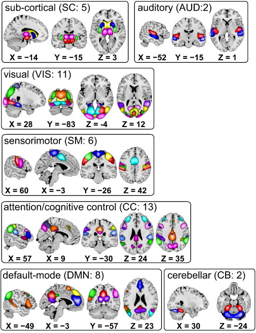
Composite maps of the 47 identified intrinsic connectivity networks (ICNs), sorted into seven subcategories. Each color in the composite maps corresponds to a different ICN. Component labels and peak coordinates are provided in Table 1.

2.6. Static functional network connectivity (sFNC)

We computed functional network connectivity (FNC), defined as pairwise correlation between ICN time courses, as a measure of average connectivity among different ICNs during the scan duration. In this work, the FNC computed using the whole ICN time courses is referred to as stationary or static FNC (sFNC). Since correlation among brain networks is primarily shown to be driven by low frequency fluctuations in BOLD fMRI data (Cordes et al., 2001), we band pass filtered the processed ICN time courses between [0.01–0.15] Hz using 5th order Butterworth filter prior to computing FNC between ICNs. The mean sFNC matrix was computed over subjects. The mean sFNC matrix was initially organized into modular partitions using the Louvain algorithm of the brain connectivity toolbox (https://sites.google.com/site/bctnet/). The modular partitions obtained from the algorithm were slightly rearranged to match the order of sFNC matrix rows to our recent work (Allen et al., 2012). After this ordering, the rows of sFNC matrix were partitioned into sub-cortical (SC), auditory (AUD), visual (VIS), sensorimotor (SM), a broad set of regions involved in cognitive control (CC) and attention, default-mode network (DMN) regions, and cerebellar (CB) components as shown in Fig. 1.

Following our earlier work, we used a MANCOVA framework (Allen et al., 2011) with backward selection to assess group differences in sFNC between ICNs. In addition to diagnosis, we used gender and site as factors, age as a covariate, as well as interactions of age by diagnosis and gender by diagnosis. Additionally, we included mean framewise displacement, (meanFD) as nuisance covariate to account for any residual motion related variance in ICA derived measures, as suggested by recent studies investigating the effects of microhead movements on functional connectivity measures (Satterthwaite et al., 2013; Yan et al., 2013). At each step, the multivariate model compared the variance explained in the response variable by the current full model to a reduced model (obtained by dropping one term and any associated interactions) using the Wilks' Lambda likelihood ratio test statistic (Christensen, 2001). In each iteration of model reduction, the least significant term that does not meet α = 0.01 threshold for the F-test is removed. The final reduced model contains all the terms and their interaction terms (if any) if the main effect or its interaction term meets the threshold. Subsequent univariate tests are performed using the final reduced model. The univariate results are presented along with the false discovery rate (FDR) multiple comparison correction threshold of p_FDR = 0.05. The sFNC results are summarized in Fig. 2.

Fig. 2.

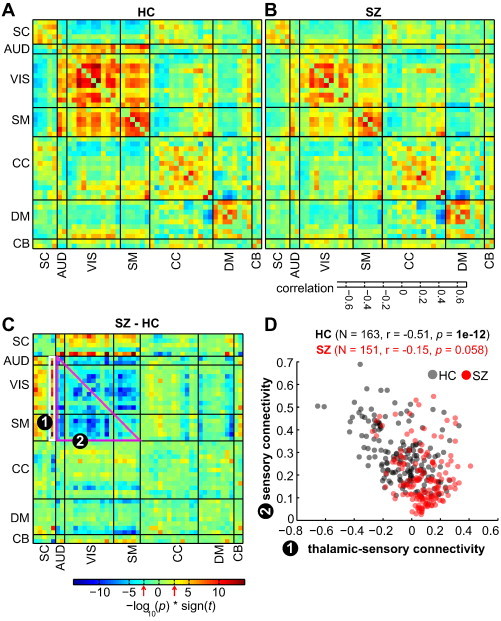
(A–B) Mean static functional network connectivity (sFNC) map for healthy controls (A) and patients with schizophrenia (B) after correcting for age, gender and meanFD. Thick black lines partition the FNC maps into the seven subcategories depicted in Fig. 1. The seven subcategories into which the ICNs are partitioned into are: sub-cortical (SC), auditory (AUD), visual (VIS), sensorimotor (SM), cognitive control (CC) and attention, default-mode network (DMN), and cerebellar (CB) components. C) The group difference (SZ–HC) in sFNC. Values are plotted as −log10(p-value) × sign(t-statistic), where statistics are obtained from the diagnosis term in univariate multiple regression models (see SI methods). The FDR threshold (q < 0.05) is depicted on the color bar with red arrows. D) Covariation between thalamic-sensory (AUD, VIS, SM) connectivity and sensory connectivity. Thalamic-sensory connectivity is defined as the average correlation between the thalamic network and all AUD, VIS and SM networks (average of cells within white rectangle labeled (1)); sensory connectivity is defined as the average correlation between all AUD, VIS, and SM ICNs (average of cells within magenta rectangle labeled (2)). Correlation between thalamic-sensory connectivity and sensory connectivity is more pronounced in HC (black circles) compared to SZ (red circles).

2.7. Dynamic functional network connectivity (dFNC)

As recent studies both in animals and humans have highlighted the nonstationary nature of functional connectivity in BOLD fMRI data (Chang and Glover, 2010; Hutchison et al., 2013), we sought to determine whether the observed sFNC differences were primarily driven by certain connectivity configurations (Hutchison et al., 2013a). Following our recent work (Allen et al., 2012), dynamic FNC (dFNC) between two ICA time courses was computed using a sliding window approach with a window size of 22 TR (44 s) in steps of 1 TR (Fig. 3A). As in our earlier work, the window constituted a rectangular window of 22 time points convolved with Gaussian of sigma 3 TRs to obtain tapering along the edges. Since estimation of covariance using time series of shorter length can be noisy, we estimated covariance from regularized inverse covariance matrix (ICOV) (Smith et al., 2011; Varoquaux et al., 2010) using the graphical LASSO framework (Friedman et al., 2008). We imposed an additional L1 norm constraint on the inverse covariance matrix to enforce sparsity. The regularization parameter was optimized for each subject by evaluating the log-likelihood of unseen data of the subject in a cross-validation framework. It has recently been reported that the original graphical LASSO implementation might not ensure positive semi-definiteness of the estimated covariance matrix (Mazumder and Hastie, 2012) and so we verified that all of the eigenvalues of the estimated dynamic covariance matrices estimated are positive. After computing dFNC values for each subject, these covariance values were Fisher-Z transformed and residualized with respect to age, gender and site using the reduced model determined from our sFNC analysis.

Fig. 3.

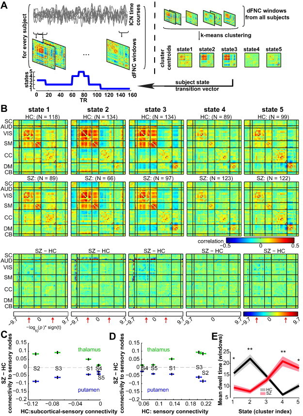
A) Schematic depicting the computation of the state transition vector for each subject. First, dFNC matrices are computed on windowed portions of the ICN time courses. Then, dFNC matrices from all subjects are clustered using the k-means algorithm, yielding cluster centroids and cluster membership assignment for all windows. When viewed in time, the window membership represents the state transition vector. B) The medians of cluster centroids by state for HC (top) and SZ (middle) along with the count of subjects that had at least one window in each state are shown. The bottom row shows the results of two sample t-test results performed across subject median dFNC maps by state, with the FDR threshold (q < 0.05) indicated by red arrows. (C–D) Illustration of the dependence of group differences on connectivity states/patterns. In (C), the group difference (SZ–HC) in thalamic-sensory connectivity, and putamen–sensory connectivity are plotted as a function of subcortical-sensory antagonism (average of cells within subcortical to sensory nodes) found in each state averaged over HC. In (D), the same group differences are displayed as a function of sensory connectivity. The error bars in (C–D) are obtained using bootstrap resampling. E) The mean ± standard error of dwell times by state for HC (black) and SZ (red). Asterisks indicate p < 0.05 (FDR corrected) and double asterisks indicate p < 0.001 (FDR corrected), as obtained via two-sample t-tests.

2.8. Clustering

Based on our observation that patterns of dFNC connectivity patterns reoccur within subjects across time and also across subjects, we used a k-means algorithm to cluster these dynamic FNC windows, partitioning the data into a set of separate clusters so as to maximize the correlation within a cluster to the cluster centroid. Instead of clustering all of the dFNC windows across all subjects, initial clustering was performed on a subset of windows from each subject, called subject exemplars hereafter, corresponding to windows of maximal variability in correlation across component pairs. To obtain the exemplars, we first compute variance of dynamic connectivity across all pairs at each window. We then select windows corresponding to local maxima in this variance time course. This resulted in an average of 8 subject exemplar windows per subject (range: 4–13). The optimal number of centroid states was estimated using the elbow criterion, defined as the ratio of within cluster to between cluster distances. A k of 5 was obtained using this method in a search window of k from 2 to 9. The correlation distance metric was chosen as it is more sensitive to the connectivity pattern irrespective of magnitude (although choosing other distance functions such as L1 distance did not make a difference in observed results). These sets of initial group centroids were used as a starting point to cluster all of the dFNC windows from all subjects.

2.9. Group differences in dynamic connectivity

We computed a subject median (computed element-wise) for each partition from the subject windows that were assigned to that partition as a representative pattern of connectivity of the subject for that state. To investigate if the observed effects of diagnosis on sFNC are primarily driven by certain dynamic FNC states, we used these subject medians for each state and evaluated the differences using a two sample t-test in a univariate manner. All of the results reported correspond to a false discovery rate multiple comparison correction threshold q < 0.05.

Using these subject state vectors, we also computed average dwell times in each state and also probability of transitioning from one state to another. Group differences in dwell times in each state as well as in probability of transition between states were also evaluated using two sample t-tests. We did not observe any significant differences in probability of transition between states across subjects.

2.10. Relationship between low frequency power and connectivity

Given the state-specific differences in connectivity between SC and AUD, VIS, and SM regions and recent findings on the influence of amplitude of low frequency fluctuations on local and long range functional connectivity measures (Di et al., 2013), we performed a post-hoc analysis evaluating the relationship between power of each SC ICN and its connectivity by state. To perform this analysis, for every subject, we computed the power spectrum of each SC ICN time course in the low frequency range (0.023–0.08 Hz; the lower threshold corresponds to the slowest frequency resolved by 44 s window) within each dynamic state, as well as the mean of the subjects' FNC connectivity between the SC node and sensory ICNs as a measure of its connectivity strength (Fig. 4A). To assess the group difference in the relationships between LF power of a component and its connectivity to sensory ICNs, robust regression models were fit for each SC component, predicting SC-sensory connectivity as a function of LF power, diagnosis, and a diagnosis-by-LF power interaction.

Fig. 4.

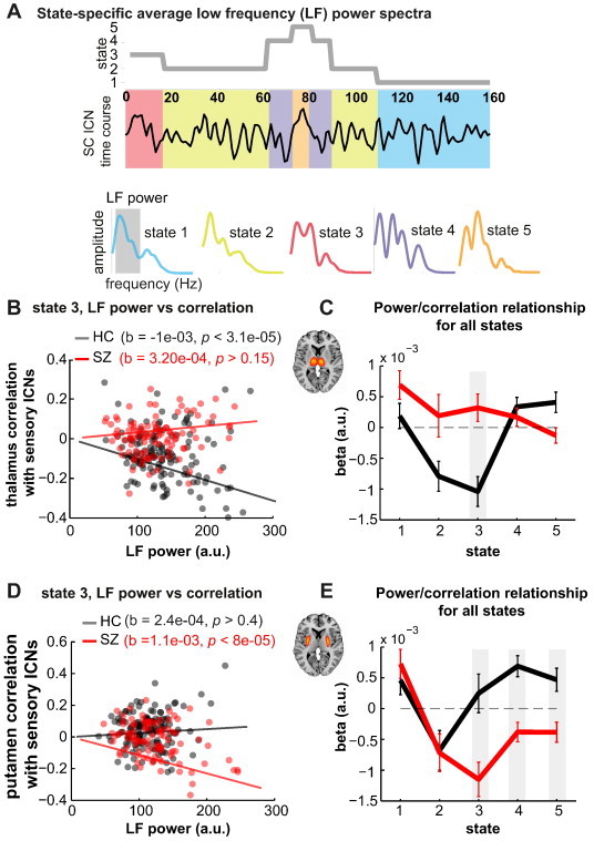
A) Schematic depicting the computation of state-specific average low frequency (LF) power spectra. A power spectrum is computed for each window (22 TRs) of an ICN time course and the spectra corresponding to the same state (obtained from subject state transition vector) are averaged together to obtain the power spectrum for that state and ICN. LF power is defined as the area under the curve in the low frequency range (0.023–0.08 Hz). B) Scatter plot showing the relationship between thalamic LF power from state 3 and state 3 thalamic-sensory connectivity for HC (black circles) and SZ (red circles). Robust fit least square regression lines are also plotted. C) Slopes estimating the linear relationship between thalamic LF power and thalamic-sensory connectivity for all states. Shaded gray area denotes a significant difference in slopes between groups (p < 0.05, FDR corrected). D) and E) show the same relationships for putamen LF power and putamen–sensory connectivity.

3. Results

Eyes-closed resting state fMRI scans from 151 SZ patients and 163 age- and gender matched healthy controls were obtained as part of the multi-site fBIRN project (Potkin and Ford, 2009). Following previous investigations of whole-brain functional connectivity (Allen et al., 2012), intrinsic connectivity networks (ICNs) and their associated time courses were decomposed using spatial ICA (Fig. 1, Table 1). Forty seven ICNs are broadly categorized based on anatomy and prior knowledge of their function into the following sub-categories: subcortical (SC), auditory (AUD), visual (VIS), somatomotor (SM), cognitive control (CC) processes, default-mode (DMN), and cerebellar (CB) networks. To characterize group differences in functional connectivity, we examined both the static functional network connectivity (sFNC), defined as temporal correlation between ICNs computed using the whole ICN time course and representing average connectivity between the networks (Jafri et al., 2008), and the dynamic FNC (dFNC), computed using a sliding-window and clustering approach, capturing the changes in connectivity throughout the scan (Allen et al., 2012).

Table 1.

Peak activations of ICN spatial maps for high model order decomposition. The quality index I_q associated with each ICN is listed in parentheses adjacent to the component number.

	BA	Nv	Tmax.	Coordinate
Sub-cortical networks
IC 75 (0.97)
Bi substantia nigra		317	31.6	–15, –15, –9
IC 1 (0.97)
R putamen		327	63.3	24 12,–3
L putamen		288	58.8	–24, 12, –6
IC 13 (0.98)
Bi caudate		665	50.6	–9, 18, 0
IC 2 (0.98)
R globus pallidum		293	56.7	30, –6, 0
L globus pallidum		275	51.6	–30, –6.3
IC 18 (0.98)
Bi thalamus		534	55.3	–9, –15, 3
Auditory networks
IC 58 (0.97)
L Heschl's gyrus	41	440	38.3	–36, –30, 12
R superior temporal gyrus	22	359	36.9	51, –15, 3
IC 51 (0.97)
R middle temporal gyrus	21	440	32.6	63, –15, –9
L middle temporal gyrus	21	300	30.4	–60, –18, –6
Visual networks
IC 91 (0.93)
R lingual gyrus	19	277	29.9	27, –66, –6
IC 57 (0.98)
L parahippocampal gyrus	37	234	37.5.0	–24, –45, –12
R parahippocampal gyrus	37	206	39.3	30, –45, –12
IC 42 (0.98)
R middle temporal gyrus	39	325	42.4	51, –69, 6
L middle occipital gyrus	37	201	33.8	–45, –72, 6
IC 60 (0.98)
R precuneus	19	357	39.8	30, –78, 33
L cuneus	19	278	33.6	–27, –78, 27
IC 20 (0.98)
R Middle Frontal gyrus	10	332	31.2	–30, –93, –6
L superior frontal gyrus	10	278	29.4	30, –90, 5
IC 76 (0.98)
Left lingual gyrus	18	802	41.7	–9, –78, –6
IC 78 (0.98)
R cuneus	18	949	29	3, –87, 21
IC 80 (0.97)
R middle temporal gyrus	22	414	38.4	54, –51, 12
L middle temporal gyrus	22	185	28.1	–54, –51, 9
IC 7 (0.98)
R cuneus	17	855	54.4	3, –84, 6
IC 43 (0.98)
R calcarine gyrus	30	952	23.2	15, –63, 9
IC 24 (0.97)
R Superior parietal lobule	7	768	25.3	–32, –88, –1
Somatomotor networks
IC 59 (0.98)
R postcentral gyrus	3	240	32.4	63, –15, 27
L postcentral gyrus	3	212	31.4	–60, –18, 33
IC 9 (0.98)
L medial frontal gyrus	6	823	51.9	42, –21, 54
IC 6 (0.97)
Right postcentral gyrus	3	622	39.8	42, –21, 54
IC 10 (0.98)
L precentral gyrus	4	598	39.6	–36, –24, 51
IC 5 (0.98)
R precentral gyrus	6	328	47.4	54, –6, 27
L precentral gyrus	6	288	49.6	–54, –9, 30
IC 74 (0.98)
L SMA	4	553	38.6	0, 0, 48
Cognitive control networks
IC 63 (0.97)
L fusiform gyrus	37	236	35.6	–42, –57, –12
R fusiform gyrus	37	89	28.1	45, –54, –12
IC 65 (0.97)
R inferior frontal gyrus	46	278	30	51, 39, 3
L inferior frontal gyrus	46	203	31.4	–45, 39, 3
IC 28 (0.98)
R inferior frontal gyrus	47	244	47.5	33, 24, –6
L inferior frontal gyrus	47	180	41.6	–33, 24, –6
IC 89 (0.91)
L supramarginal gyrus	40	293	37.3	–54, –57, 36
R supramarginal gyrus	40	288	38.7	60, –51, 9
IC 35 (0.92)
L precuneus	7	506	46.5	–6, –72, 39
R cingulate gyrus	23	120	39.9	3, –27, 27
IC 21 (0.98)
R middle frontal gyrus	10	332	31.2	33, 54, 12
L superior frontal gyrus	10	278	29.4	–33, 45, 21
IC 47 (0.98)
Cingulate gyrus	23	621	47.4	0, –36, 27
IC 94 (0.97)
R inferior parietal lobule	40	374	34.9	–42, –42, 45
IC 66 (0.98)
R inferior parietal lobule	40	510	41.2	42, −45, 48
IC 34 (0.95)
R inferior frontal gyrus	9	244	32.2	42, 9 30
L middle frontal gyrus	9	180	32.7	–45, 12 30
IC 40 (0.97)
Precuneus	7	661	50.4	0, –60, 48
IC 41 (0.96)
R insula	13	325	41	45, –3, 0
L insula	13	188	33.3	–45, 0, 3
IC 96 (0.96)
R inferior parietal loble	40	200	34.1	57, –30, 24
L inferior parietal loble	40	98	27.9	–60, –36, 24
Default-mode networks
IC 30 (0.93)
Precuneus	7	641	58.2	0, –57, 33
IC 53 (0.98)
L anterior cingulate gyrus	32	742	43.5	–3, 48, 12
IC 69 (0.97)
R medial frontal gyrus	8	443	45.8	3 2042, 45
IC 95 (0.97)
L angular gyrus	40	555	43	–48, –63, 42
IC 84 (0.98)
R angular gyrus	40	443	45.8	51, –60, 39
IC 90 (0.98)
R angular gyrus	39	213	36.1	45, –75, 30
L superior occipital gyrus	19	89	26.6	–36, –81, 30
IC 61 (0.74)
L middle temporal gyrus	22	197	29.3	–57, –42, 0
R inferior frontal gyrus	44	195	32.6	–54, 15 6
IC 12 (0.98)
L precuneus	30	729	57.1	–12, –57, 15
Cerebellar networks
IC 46 (0.97)
L culmen		182	32.2	–24, –42, –24
R culmen		171	33.8	27, –48, –24
IC 88 (0.97)
R declive		870	39.4	30, –75, –24

BA = Brodmann area; Nv = number of voxels in each cluster; T_max. = maximum t-statistic in each cluster; Coordinate = max coordinate (mm) in MNI space, following LPI convention.

3.1. Group differences in static FNC

Group differences in sFNC were evaluated with a MANCOVA statistical model with backward selection (Allen et al., 2011), treating gender, diagnosis, and site as factors of interest, age as a covariate, and mean framewise displacement (meanFD, mean of absolute frame to frame head motion assuming 50 mm head radius) as a nuisance covariate. Interactions between age and gender, and age and diagnosis were also included. The final terms retained in the model after backward selection using an alpha level of 0.01 included diagnosis (Hotelling's T = 214.9, < 1e−16), site (T = 213.0, p < 1e−13), age (T = 117.0, p < 2e−11), meanFD (T = 77.0, p < 2e−9), and an age-by-diagnosis interaction (T = 32.0, p < 5e−3). Subsequent univariate tests were performed using a reduced model with these terms. The group-specific mean sFNC matrices are shown in Fig. 2A–B along with the group difference (Fig. 2C), after residualizing with respect to gender, site and meanFD. Since the effect of diagnosis was tested with the age-by-diagnosis term included in the model, the diagnosis effect corresponds to differences at the mean age across groups. Repeating the analysis after dropping the age-by-diagnosis interaction term revealed an identical set of significant sFNC pairs, indicating sFNC differences in diagnosis are present across the age span studied for all ICN pairs that showed significant group differences5^*. Compared to the HC, the SZ group showed significantly weaker connectivity between all AUD, SM and VIS networks. Additionally, the SZ group showed hyperconnectivity between SC networks (particularly the thalamus) and AUD, VIS and SM cortical networks. As depicted in Fig. S1A and Fig. S1B, these group differences are consistent across all the sites with reasonably high effect sizes (Cohen's D range: [–1.5 1.5]).

Based on the observation of high within network connectivity among sensory (AUD, VIS and SM) ICNs and their inverse correlation to the thalamus, we tested if these two patterns covary across subjects. In Fig. 2D, we show that the mean strength of thalamic connectivity to sensory nodes (average of cells in white rectangle labeled (1) and referred to as thalamic-sensory connectivity) covaries with the strength of mean connectivity within these sensory ICNs (average of cells in magenta triangle labeled (2) and referred to as sensory connectivity) in an inverse manner that is much more pronounced in healthy controls than SZ patients.

To determine whether current medication could account for the observed sFNC differences related to diagnosis, we repeated the analysis after regressing out medication (summarized as chlorpromazine equivalence scores) from patient sFNC values. We found similar group differences (T = 195.3, p < 1e−16). Additional MANCOVA tests within the patient group investigating the effects of symptom scores (positive and negative symptom scores (PANSS), and general psychopathology scale) on sFNC measures revealed no significant associations. To determine whether the observed differences between the groups were largely a reflection of duration of chronic illness in patients per se, we regressed out duration of illness from the patient sFNC values and evaluated the effect of diagnosis using the MANCOVA model. The effect of diagnosis remained very significant (T = 184.9, p < 1e−15).

3.2. Group differences in dynamic FNC

The group-specific medians for each state are shown in Fig. 3B (top two rows). States 1, 2 and 3 show moderate to high correlation among the VIS, MOT and AUDICNs. In states 2 and 3, sub-cortical regions as well as a set of ICNs in CC category show antagonism with AUD, SM, and VIS ICNs as compared to state 1. State 3 distinguishes itself from state 2 with respect to connectivity of default mode ICNs; connectivity within default mode regions is stronger and also more anticorrelated from sensory and motor regions in state 3. State 4 shows a weak connectivity within each subcategory and demonstrates no strong connectivity between subcategories. State 5 is similar to state 4 except that the connectivity of default mode ICNs resembles that of state 3.

The group differences in dFNC among five identified connectivity states are shown in Fig. 3B (bottom row). Note that not all subjects have dynamic windows that are assigned to every state, thus the number of observations (subject-specific matrices, and therefore degrees of freedom in the model) changes with each state (see subject counts per state shown in Fig. 3B). Examining group differences by state demonstrates that the observed hyperconnectivity between the thalamus and sensory ICNs in patients with SZ occurs primarily during states 2 and 3, in which there is greater cortical–subcortical antagonism and when the sensorimotor networks are highly synchronized. To depict these relationships visually, we plot thalamic to sensory ICN hyperconnectivity as a function of each state's sensory-subcortical connectivity, computed by averaging dFNC between subcortical regions and sensory ICNs in Fig. 3C, and each state's average within sensory network connectivity in Fig. 3D, computed by averaging the dFNC values between sensory networks. In addition to the thalamus, dFNC analysis reveals that posterior putamen ICN is the only node among SC regions in which patients with SZ show hypoconnectivity with AUD, VIS and SM regions compared to HC; this hypoconnectivity is also more pronounced in states 2 and 3 where the thalamus shows hyperconnectivity (Fig. 3C and 3D). Subsequent tests investigating the association between thalamic hyperconnectivity and putamen hypoconnectivity revealed that these do not covary across subjects (r = 0.002 and 0.13 for states 2 and 3 respectively), suggesting distinct mechanisms.

An examination of the proportion of subject windows assigned to each state suggests that patients with SZ, in general, spend significantly more time in relatively more sparsely connected state 4, and less time in states 1 and 2 (Fig. 3E). Compared to HC, patients make fewer transitions to states 1 and 2, dwell in these states for much shorter duration, and make more transitions to states 4 and 5, as well as stay longer in these states. The dwell time patterns were consistent across all sites (Fig. S2). Even though patients dwell longer in states 4 and 5, the thalamic and sensory connectivity differences observed in sFNC are not pronounced during these states. Also, fewer patients transition into states 1, 2 and 3 compared to healthy controls suggesting variability in sFNC differences from smaller samples may well be determined by the probability that they transition into certain states.

To test whether the observed effects were related to wakefulness, the k-means clustering was repeated for dFNC windows corresponding to the first and second half of scan sessions separately. Consistent results were obtained regarding both the percent of windows assigned to each state, as well as in the state-specific group differences observed (albeit with a reduced strength in observed connectivity differences due to using 50% of the data), suggesting that the observed differences are not strongly driven by wakefulness, which would be expected to decrease during the scan.

Tests on association between SC nodes and their connectivity to sensory networks revealed that during states 2 and 3, HC demonstrate a significant negative slope between the thalamus power spectra and its connectivity to sensory ICNs, meaning that larger low frequency thalamic signal fluctuations are associated with greater anti-correlation with sensory areas. In contrast, patients show the opposite (state 3) or reduced (state 2) trend (Fig. 4C). The individual subject values for state 3 are shown in Fig. 4B. In addition to the thalamus, posterior putamen also showed group differences in the relationship between low frequency power and connectivity. In patients, greater low frequency power was associated with stronger putamen–sensory anti-correlation, however this trend was absent or reversed in states 3, 4, and 5 for healthy controls.

4. Discussion

In this study, we investigated the differences in functional connectivity dynamics during eyes closed resting between HC and SZ patients. Our analysis suggests that, compared with controls, patients show (1) hyperconnectivity between the thalamus and sensory networks, (2) reduced connectivity between auditory, sensorimotor and visual networks and (3) most pronounced abnormalities during connectivity states that exhibit cortical–subcortical antagonism and states of increased connectivity within sensory ICNs. Furthermore, the relationship between thalamic low frequency power and thalamocortical connectivity is altered during these connectivity states in SZ, with patients showing weak positive connectivity with greater power between the thalamus and sensory networks while healthy controls show inverse relationship between the two.

4.1. Thalamus dysconnectivity in schizophrenia

The observed hyperconnectivity between the thalamus and sensory ICNs in patients with SZ in sFNC is consistent with and significantly extends recent reports using seed-based connectivity approaches. By investigating connectivity of thalamic voxels to non-overlapping cortical seeds (Woodward et al., 2012), Woodward and colleagues showed that compared to HC, patients with SZ show stronger connectivity between the thalamus and motor/somatosensory regions while the connectivity between the thalamus and prefrontal cortex is lower. In a recent report using seed-based functional connectivity analysis, Anticevic and colleagues (Anticevic et al., 2013) demonstrate similar hyperconnectivity between the thalamus and sensory-motor cortices and hypoconnectivity between the thalamus and prefrontal–striatal–cerebellar regions in a large sample of patients with SZ. They also demonstrate interplay between nodes that show hypoconnectivity with the thalamus and nodes that demonstrate hyperconnectivity with the thalamus: In both healthy controls and patients with SZ, subjects that showed the lowest thalamo-prefrontal-cerebellar coupling were the ones that showed the highest thalamo-sensory-motor coupling and the strength of this coupling was much weaker in patients compared to controls. In our static FNC results, we replicate this finding (Fig. S3A) and in addition show that coupling within sensory-motor regions and cortical–subcortical antagonism co-occurs with this thalamic hyperconnectivity (Fig. S3B). Investigations of structural connectivity support these findings. Marenco and colleagues have shown higher total structural connectivity between the thalamus and sensory motor regions along with lower structural connectivity between the thalamus and prefrontal cortex using diffusion tensor imaging data (Marenco et al., 2011).

In addition to the thalamus hyperconnectivity, our sFNC results also suggest hypoconnectivity between AUD, VIS and SM ICNs in patients. This, apparently novel, finding is present in data from almost all sites, suggesting a robust and reproducible effect that should be explored in future work. The identification of this group difference, along with connectivity differences related to subcortical areas, speaks to the strength of our whole-brain, data-driven approach, which is not limited by the selection of specific seeds or regions of interest.

Although stationary analyses of FC do reveal significantly altered connectivity patterns in patients with SZ, it is critical to determine whether these differences persist throughout time, regardless of the mental activity in which subjects are engaged, or arise only during certain brain states. Using a dynamic analysis based on sliding windows and k-means clustering, we identified five different connectivity patterns (see Fig. 3), and found that the thalamus hyperconnectivity in patients is primarily observed in states that depict cortical–subcortical antagonism along with stronger connectivity within sensory ICNs. This antagonism between cortical and subcortical regions has been observed during descent to sleep, along with a breakdown of connectivity among default-mode regions (Larson-Prior et al., 2009; Spoormaker et al., 2010) with an increase in functional modularity (Boly et al., 2012). Similar functional connectivity states have been associated with slowing of EEG oscillations in simultaneous EEG–fMRI recordings (Allen et al., 2013). We speculate that during unconstrained state of eyes closed condition, connectivity patterns in state 2 might correspond to the descent into light sleep or drowsiness.

4.2. Advantages of a dynamic approach

The consistency of observed static connectivity differences or lack thereof between groups across independent studies could well be attributed to differences in the mental states during which subjects are scanned. In our multi-site study, patients with SZ spent significantly longer duration in weakly connected state 4 and tended to make fewer transitions to states that show cortical–subcortical antagonism; group differences in transitions show remarkable consistency across sites (see Fig. S2). Whether the observed differences in dwell times across states or the differences in connectivity strengths in a given state are more critical needs to be determined.

Given that the resting state data were collected in eyes closed state, one could argue that the observed sFNC group differences might be driven by differences in wakefulness between groups. Investigating these FC differences dynamically makes this less problematic as group differences in connectivity are computed from similar connectivity states obtained from data-driven clustering assignment. Also these state specific functional connectivity differences were prevalent during both halves of the rest scan suggesting that the observed differences may not be explained just by differences in wakefulness.

Furthermore, it has been suggested that functional connectivity measures computed as statistical association between networks over 5 or more minutes stabilize (Van Dijk et al., 2010) and follow anatomical connectivity (Deco et al., 2011). This measure of average connectivity, although useful, might not be enough to fully characterize the dynamically changing association between networks which is thought to be critical to process, coordinate, integrate and respond to internal and external stimuli (Hutchison et al., 2013). In the current analysis, the observed hypoconnectivity of putamen ICN with sensory ICNs in patients is more apparent in dynamic analysis and is not significant in sFNC analysis as this effect is specific to certain states.

4.3. Limitations and future directions

4.3.1. Future directions

The thalamus is a crucial node involved in transmitting, processing, communicating and integrating neuronal signals and composed of anatomically distinct sub-nuclei with different functional properties (Byne et al., 2009). Recent functional imaging studies reporting thalamo-cortical informational flow disruptions in patients with SZ have used either anatomically predefined ROI's within the thalamus (for example medio-dorsal nucleus ROI in Welsh et al., 2010) or data driven clustering of voxels within the thalamus based on their connectivity (Anticevic et al., 2013; Woodward et al., 2012) to further localize the perturbation within the thalamus. In our group ICA framework, the thalamus manifests as a single ICN and further localization of the observed disconnectivity in the thalamus can provide greater insights into the observed connectivity differences.

Also patients with SZ have been shown to have deficits in thalamic reticular nucleus neurobiology which plays an important role in top down processes such as attentional modulation as well as bottom up processes such as sensory gating and generation of sleep spindles (brief bursts of 12–16 Hz oscillations in EEG) during descent to sleep (Ferrarelli and Tononi, 2011). Additional experiments using simultaneous EEG–fMRI may help us understand what processes the observed state-specific connectivity differences in patients correspond to.

4.3.2. Limitations

Although we partially replicate the whole brain dynamic connectivity patterns observed in our earlier study performed on healthy controls (Allen et al., 2012), it is still unclear whether the observed connectivity patterns are of neural origin, or whether they are merely spurious patterns induced by non-neural sources. Although recent evidence from animals and humans has demonstrated links between FC dynamics and neural activity (Pan et al., 2013) as well as FC dynamics and behavioral variability (Fox and Raichle, 2007), reports have also highlighted the pitfall of over-interpreting fluctuations in FC as having a neural origin, when in fact these fluctuations can arise from basic BOLD signal properties (Handwerker et al., 2012; Hutchison et al., 2013; Keilholz et al., 2013). There is perhaps less concern for spurious findings in the current work due to our multivariate clustering approach, which we show in a control analysis using synthetic data where ICN time courses have been phase randomized in the Fourier domain. The phase randomized data yielded cluster centroids that did not have any modular structure, suggesting that the observed structure in connectivity patterns requires intact phase relationships across different nodes of the brain (Fig. S4 and Supplementary methods S2). Notably, this is not the case in univariate analyses that use measures of correlation variability (such as the standard deviation or Fourier power) as proxies for dynamics (Handwerker et al., 2012; Keilholz et al., 2013).

Recent neuroimaging studies have highlighted the importance of controlling for small micromovements of subjects' heads during the scan session, as such movements are shown to influence the functional connectivity metrics differently with distance between nodes (Power et al., 2012). In lieu of these concerns, the sFNC analysis was repeated with select few subjects that had a mean framewise displacement of less than 0.2 mm, and the dFNC analysis was performed on select windows after discarding any dynamic window segment that had a micromovement greater than 0.5 mm. In both analyses, the group differences in sFNC (Fig. S5), the centroids of clustered dFNC states as well the differences in dwell times in each state remained similar to the results obtained using all of the data (Fig. S6).

The patients with SZ were medicated and many have a history of alcohol and drug abuse, both of which might have an impact on observed group differences. Although the observed group differences in connectivity remain significant even after regressing out chlorpromazine equivalence scores of current medication from patient group, the effect of different medications cannot be equated as the underlying mechanism of the typical and atypical antipsychotics is quite different. Furthermore, long term effects of medication cannot be accounted for given the known impact of these medications on brain structure (Moncrieff and Leo, 2010) although regressing out duration of illness as a proxy did not have any impact on observed differences. Similar analysis on data from non-medicated first episode SZ patients would provide better insights into the primary causes of observed disturbances in FNC.

Appendix A. Supplementary data

Supplementary material.

References

- Allen E.A., Damaraju E., Plis S.M., Erhardt E.B., Eichele T., Calhoun V.D. Tracking whole-brain connectivity dynamics in the resting state. Cerebral Cortex. 2012;24(3):663–676. doi: 10.1093/cercor/bhs352. [DOI] [PMC free article] [PubMed] [Google Scholar]
- Allen E.A., Eichele T., Wu L., Calhoun V.D. EEG Signature of Functional Connectivity States. Organization of Human Brain Mapping; Seattle: 2013. [Google Scholar]
- Allen E.A., Erhardt E.B., Damaraju E., Gruner W., Segall J.M., Silva R.F., Havlicek M., Rachakonda S., Fries J., Kalyanam R., Michael A.M., Caprihan A., Turner J.A., Eichele T., Adelsheim S., Bryan A.D., Bustillo J., Clark V.P., Feldstein Ewing S.W., Filbey F., Ford C.C., Hutchison K., Jung R.E., Kiehl K.A., Kodituwakku P., Komesu Y.M., Mayer A.R., Pearlson G.D., Phillips J.P., Sadek J.R., Stevens M., Teuscher U., Thoma R.J., Calhoun V.D. A baseline for the multivariate comparison of resting-state networks. Frontiers in Systems Neuroscience. 2011 doi: 10.3389/fnsys.2011.00002. [DOI] [PMC free article] [PubMed] [Google Scholar]
- Bell A.J., Sejnowski T.J. An information-maximization approach to blind separation and blind deconvolution. Neural Computation. 1995;7:1129–1159. doi: 10.1162/neco.1995.7.6.1129. 7584893 [DOI] [PubMed] [Google Scholar]
- Anticevic A., Cole M.W., Repovs G., Murray J.D., Brumbaugh M.S., Winkler A.M., Savic A., Krystal J.H., Pearlson G.D., Glahn D.C. Characterizing thalamo-cortical disturbances in schizophrenia and bipolar illness. Cerebral Cortex. 2013 doi: 10.1093/cercor/bht165. [DOI] [PMC free article] [PubMed] [Google Scholar]
- Bleuler E. Dementia Praecox or the Group of Schizophrenias. International Universities Press; New York: 1950. [Google Scholar]
- Boly M., Perlbarg V., Marrelec G., Schabus M., Laureys S., Doyon J., Pélégrini-Issac M., Maquet P., Benali H. Hierarchical clustering of brain activity during human nonrapid eye movement sleep. Proceedings of the National Academy of Sciences of the U.S.A. 2012;109:5856–5861. doi: 10.1073/pnas.1111133109. [DOI] [PMC free article] [PubMed] [Google Scholar]
- Breakspear M., Terry J.R., Friston K.J., Harris A.W.F., Williams L.M., Brown K., Brennan J., Gordon E. A disturbance of nonlinear interdependence in scalp EEG of subjects with first episode schizophrenia. NeuroImage. 2003;20:466–478. doi: 10.1016/s1053-8119(03)00332-x. 14527607 [DOI] [PubMed] [Google Scholar]
- Byne W., Hazlett E.A., Buchsbaum M.S., Kemether E. The thalamus and schizophrenia: current status of research. Acta Neuropathologica. 2009;117:347–368. doi: 10.1007/s00401-008-0404-0. [DOI] [PubMed] [Google Scholar]
- Calhoun V.D., Adali T., Pearlson G.D., Pekar J.J. A method for making group inferences from functional MRI data using independent component analysis. Human Brain Mapping. 2001;14:140–151. doi: 10.1002/hbm.1048. 11559959 [DOI] [PMC free article] [PubMed] [Google Scholar]
- Calhoun V.D., Sui J., Kiehl K., Turner J., Allen E., Pearlson G. Exploring the psychosis functional connectome: aberrant intrinsic networks in schizophrenia and bipolar disorder. Frontiers in Psychiatry. 2011;2:75. doi: 10.3389/fpsyt.2011.00075. 22291663 [DOI] [PMC free article] [PubMed] [Google Scholar]
- Chang C., Glover G.H. Time-frequency dynamics of resting-state brain connectivity measured with fMRI. NeuroImage. 2010;50:81–98. doi: 10.1016/j.neuroimage.2009.12.011. 20006716 [DOI] [PMC free article] [PubMed] [Google Scholar]
- Christensen R. Advanced Linear Modeling: Multivariate, Time Series, and Spatial Data; Nonparametric Regression and Response Surface Maximization. Springer; 2001. [Google Scholar]
- Cordes D., Haughton V.M., Arfanakis K., Carew J.D., Turski P.A., Moritz C.H., Quigley M.A., Meyerand M.E. Frequencies contributing to functional connectivity in the cerebral cortex in “resting-state” data. AJNR. American Journal of Neuroradiology. 2001;22:1326–1333. 11498421 [PMC free article] [PubMed] [Google Scholar]
- Cribben I., Haraldsdottir R., Atlas L.Y., Wager T.D., Lindquist M.A. Dynamic connectivity regression: determining state-related changes in brain connectivity. Neuroimage. 2012;61:907–920. doi: 10.1016/j.neuroimage.2012.03.070. 22484408 [DOI] [PMC free article] [PubMed] [Google Scholar]
- Deco G., Jirsa V.K., McIntosh A.R. Emerging concepts for the dynamical organization of resting-state activity in the brain. Nature Reviews. Neuroscience. 2011;56:2043. doi: 10.1038/nrn2961. [DOI] [PubMed] [Google Scholar]
- Deco G., Ponce-Alvarez A., Mantini D., Romani G.L., Hagmann P., Corbetta M. Resting-state functional connectivity emerges from structurally and dynamically shaped slow linear fluctuations. Journal of Neuroscience. 2013;33:11239–11252. doi: 10.1523/JNEUROSCI.1091-13.2013. [DOI] [PMC free article] [PubMed] [Google Scholar]
- Di X., Kim E.H., Huang C.-C., Tsai S.-J., Lin C.-P., Biswal B.B. The influence of the amplitude of low-frequency fluctuations on resting-state functional connectivity. Frontiers in Human Neuroscience. 2013;7:118. doi: 10.3389/fnhum.2013.00118. 23565090 [DOI] [PMC free article] [PubMed] [Google Scholar]
- Erhardt E.B., Rachakonda S., Bedrick E.J., Allen E.A., Adali T., Calhoun V.D. Comparison of multi-subject ICA methods for analysis of fMRI data. Human Brain Mapping. 2011;32:2075–2095. doi: 10.1002/hbm.21170. 21162045 [DOI] [PMC free article] [PubMed] [Google Scholar]
- Ferrarelli F., Tononi G. The thalamic reticular nucleus and schizophrenia. Schizophrenia Bulletin. 2011;37:306–315. doi: 10.1093/schbul/sbq142. [DOI] [PMC free article] [PubMed] [Google Scholar]
- Fornito A., Zalesky A., Pantelis C., Bullmore E.T. Schizophrenia, neuroimaging and connectomics. Neuroimage. 2012;62:2296–2314. doi: 10.1016/j.neuroimage.2011.12.090. 22387165 [DOI] [PubMed] [Google Scholar]
- Fox M.D., Greicius M. Clinical applications of resting state functional connectivity. Frontiers in Systems Neuroscience. 2010;4:19. doi: 10.3389/fnsys.2010.00019. [DOI] [PMC free article] [PubMed] [Google Scholar]
- Fox M.D., Raichle M.E. Spontaneous fluctuations in brain activity observed with functional magnetic resonance imaging. Nature Reviews. Neuroscience. 2007;8:700–711. doi: 10.1038/nrn2201. 17704812 [DOI] [PubMed] [Google Scholar]
- Friedman J., Hastie T., Tibshirani R. Sparse inverse covariance estimation with the graphical lasso. Biostatistics (Oxford, England) 2008;9:432–441. doi: 10.1093/biostatistics/kxm045. 18079126 [DOI] [PMC free article] [PubMed] [Google Scholar]
- Friston K.J. The disconnection hypothesis. Schizophrenia Research. 1998;30:115–125. doi: 10.1016/s0920-9964(97)00140-0. 9549774 [DOI] [PubMed] [Google Scholar]
- Handwerker D.A., Roopchansingh V., Gonzalez-Castillo J., Bandettini P.A. Periodic changes in fMRI connectivity. Neuroimage. 2012;63:1712–1719. doi: 10.1016/j.neuroimage.2012.06.078. 22796990 [DOI] [PMC free article] [PubMed] [Google Scholar]
- Hutchison R.M., Womelsdorf T., Allen E.A., Bandettini P.A., Calhoun V.D., Corbetta M., Della Penna S., Duyn J.H., Glover G.H., Gonzalez-Castillo J. Dynamic functional connectivity: promise, issues, and interpretations. Neuroimage. 2013;80:360–368. doi: 10.1016/j.neuroimage.2013.05.079. 23707587 [DOI] [PMC free article] [PubMed] [Google Scholar]
- Hutchison R.M., Womelsdorf T., Gati J.S., Everling S., Menon R.S. Resting-state networks show dynamic functional connectivity in awake humans and anesthetized macaques. Human Brain Mapping. 2013;34:2154–2177. doi: 10.1002/hbm.22058. 22438275 [DOI] [PMC free article] [PubMed] [Google Scholar]
- Jafri M.J., Pearlson G.D., Stevens M., Calhoun V.D. A method for functional network connectivity among spatially independent resting-state components in schizophrenia. NeuroImage. 2008;39:1666–1681. doi: 10.1016/j.neuroimage.2007.11.001. 18082428 [DOI] [PMC free article] [PubMed] [Google Scholar]
- Keilholz S.D., Magnuson M.E., Pan W.-J., Willis M., Thompson G.J. Dynamic properties of functional connectivity in the rodent. Brain Connectivity. 2013;3:31–40. doi: 10.1089/brain.2012.0115. 23106103 [DOI] [PMC free article] [PubMed] [Google Scholar]
- Kraepelin E. Dementia Praecox and Paraphrenia. Krieger Publishing; 1971. [Google Scholar]
- Larson-Prior L.J., Zempel J.M., Nolan T.S., Prior F.W., Snyder A.Z., Raichle M.E. Cortical network functional connectivity in the descent to sleep. Proceedings of the National Academy of Sciences of the United States of America. 2009;106:4489–4494. doi: 10.1073/pnas.0900924106. 19255447 [DOI] [PMC free article] [PubMed] [Google Scholar]
- Liu X., Duyn J.H. Time-varying functional network information extracted from brief instances of spontaneous brain activity. Proceedings of the National Academy of Sciences of the United States of America. 2013;110:4392–4397. doi: 10.1073/pnas.1216856110. 23440216 [DOI] [PMC free article] [PubMed] [Google Scholar]
- Marenco S., Stein J.L., Savostyanova A.A., Sambataro F., Tan H.-Y., Goldman A.L., Verchinski B.A., Barnett A.S., Dickinson D., Apud J.A. Investigation of anatomical thalamo-cortical connectivity and fMRI activation in schizophrenia. Neuropsychopharmacology. 2011;37:499–507. doi: 10.1038/npp.2011.215. [DOI] [PMC free article] [PubMed] [Google Scholar]
- Mathalon D.H., Ford J.M. Divergent approaches converge on frontal lobe dysfunction in schizophrenia. American Journal of Psychiatry. 2008;165:944–948. doi: 10.1176/appi.ajp.2008.08050735. 18676596 [DOI] [PMC free article] [PubMed] [Google Scholar]
- Mazoyer B., Zago L., Mellet E., Bricogne S., Etard O., Houdé O., Crivello F., Joliot M., Petit L., Tzourio-Mazoyer N. Cortical networks for working memory and executive functions sustain the conscious resting state in man. Brain Research Bulletin. 2001;54:287–298. doi: 10.1016/s0361-9230(00)00437-8. 11287133 [DOI] [PubMed] [Google Scholar]
- Mazumder R., Hastie T. The graphical lasso: new insights and alternatives. Electronic Journal of Statistics. 2012;6:2125–2149. doi: 10.1214/12-EJS740. [DOI] [PMC free article] [PubMed] [Google Scholar]
- Moncrieff J., Leo J. A systematic review of the effects of antipsychotic drugs on brain volume. Psychological Medicine. 2010;40:1409–1422. doi: 10.1017/S0033291709992297. 20085668 [DOI] [PubMed] [Google Scholar]
- Pan W.-J., Thompson G.J., Magnuson M.E., Jaeger D., Keilholz S. Infraslow LFP correlates to resting-state fMRI BOLD signals. Neuroimage. 2013;74:288–297. doi: 10.1016/j.neuroimage.2013.02.035. 23481462 [DOI] [PMC free article] [PubMed] [Google Scholar]
- Pearlson G.D. Neurobiology of schizophrenia. Annals of Neurology. 2000;48:556–566. 11026439 [PubMed] [Google Scholar]
- Pearlson G.D., Marsh L. Structural brain imaging in schizophrenia: a selective review. Biological Psychiatry. 1999;46:627–649. doi: 10.1016/s0006-3223(99)00071-2. 10472416 [DOI] [PubMed] [Google Scholar]
- Potkin S.G., Ford J.M. Widespread cortical dysfunction in schizophrenia: the FBIRN imaging consortium. Schizophrenia Bulletin. 2009;35:15–18. doi: 10.1093/schbul/sbn159. 19023124 [DOI] [PMC free article] [PubMed] [Google Scholar]
- Power J.D., Barnes K.A., Snyder A.Z., Schlaggar B.L., Petersen S.E. Spurious but systematic correlations in functional connectivity MRI networks arise from subject motion. Neuroimage. 2012;59:2142–2154. doi: 10.1016/j.neuroimage.2011.10.018. 22019881 [DOI] [PMC free article] [PubMed] [Google Scholar]
- Sakoğlu Ü., Pearlson G.D., Kiehl K.A., Wang Y.M., Michael A.M., Calhoun V.D. A method for evaluating dynamic functional network connectivity and task-modulation: application to schizophrenia. Magnetic Resonance Materials in Physics, Biology and Medicine. 2010;23:351–366. doi: 10.1007/s10334-010-0197-8. [DOI] [PMC free article] [PubMed] [Google Scholar]
- Salvador R., Sarró S., Gomar J.J., Ortiz-Gil J., Vila F., Capdevila A., Bullmore E., McKenna P.J., Pomarol-Clotet E. Overall brain connectivity maps show corticosubcortical abnormalities in schizophrenia. Human Brain Mapping. 2010;31:2003–2014. doi: 10.1002/hbm.20993. 20225222 [DOI] [PMC free article] [PubMed] [Google Scholar]
- Satterthwaite T.D., Elliott M.a., Gerraty R.T., Ruparel K., Loughead J., Calkins M.E., Eickhoff S.B., Hakonarson H., Gur R.C., Gur R.E., Wolf D.H. An improved framework for confound regression and filtering for control of motion artifact in the preprocessing of resting-state functional connectivity data. Neuroimage. 2013;64:240–256. doi: 10.1016/j.neuroimage.2012.08.052. [DOI] [PMC free article] [PubMed] [Google Scholar]
- Smith S.M., Fox P.T., Miller K.L., Glahn D.C., Fox P.M., Mackay C.E., Filippini N., Watkins K.E., Toro R., Laird A.R., Beckmann C.F. Correspondence of the brain's functional architecture during activation and rest. Proceedings of the National Academy of Sciences of the United States of America. 2009;106:13040–13045. doi: 10.1073/pnas.0905267106. 19620724 [DOI] [PMC free article] [PubMed] [Google Scholar]
- Smith S.M., Miller K.L., Salimi-Khorshidi G., Webster M., Beckmann C.F., Nichols T.E., Ramsey J.D., Woolrich M.W. Network modelling methods for FMRI. Neuroimage. 2011;54:875–891. doi: 10.1016/j.neuroimage.2010.08.063. 20817103 [DOI] [PubMed] [Google Scholar]
- Spoormaker V.I., Schröter M.S., Gleiser P.M., Andrade K.C., Dresler M., Wehrle R., Sämann P.G., Czisch M. Development of a large-scale functional brain network during human non-rapid eye movement sleep. Journal of Neuroscience. 2010;30:11379–11387. doi: 10.1523/JNEUROSCI.2015-10.2010. [DOI] [PMC free article] [PubMed] [Google Scholar]
- Van Dijk K.R.A., Hedden T., Venkataraman A., Evans K.C., Lazar S.W., Buckner R.L. Intrinsic functional connectivity as a tool for human connectomics: theory, properties, and optimization. Journal of Neurophysiology. 2010;103:297–321. doi: 10.1152/jn.00783.2009. 19889849 [DOI] [PMC free article] [PubMed] [Google Scholar]
- Varoquaux G., Gramfort A., Poline J.-B., Thirion B. Brain covariance selection: better individual functional connectivity models using population prior. In: NIPS, editor. 2010. pp. 2334–2342. [Google Scholar]
- Welsh R.C., Chen A.C., Taylor S.F. Low-frequency BOLD fluctuations demonstrate altered thalamocortical connectivity in schizophrenia. Schizophrenia Bulletin. 2010;36:713–722. doi: 10.1093/schbul/sbn145. 18990709 [DOI] [PMC free article] [PubMed] [Google Scholar]
- Whitfield-Gabrieli S., Thermenos H.W., Milanovic S., Tsuang M.T., Faraone S.V., McCarley R.W., Shenton M.E., Green A.I., Nieto-Castanon A., LaViolette P., Wojcik J., Gabrieli J.D.E., Seidman L.J. Hyperactivity and hyperconnectivity of the default network in schizophrenia and in first-degree relatives of persons with schizophrenia. Proceedings of the National Academy of Sciences of the U.S.A. 2009;106:1279–1284. doi: 10.1073/pnas.0809141106. [DOI] [PMC free article] [PubMed] [Google Scholar]
- Woodward N.D., Karbasforoushan H., Heckers S. Thalamocortical dysconnectivity in schizophrenia. American Journal of Psychiatry. 2012;169:1092–1099. doi: 10.1176/appi.ajp.2012.12010056. [DOI] [PMC free article] [PubMed] [Google Scholar]
- Yan C.-G., Cheung B., Kelly C., Colcombe S., Craddock R.C., Di Martino A., Di, Li Q., Zuo X.-N., Castellanos F.X., Milham M.P. A comprehensive assessment of regional variation in the impact of head micromovements on functional connectomics. Neuroimage. 2013;76:183–201. doi: 10.1016/j.neuroimage.2013.03.004. 23499792 [DOI] [PMC free article] [PubMed] [Google Scholar]
Associated Data
This section collects any data citations, data availability statements, or supplementary materials included in this article.
Supplementary Materials