Abstract
Purpose
Parallel imaging allows the reconstruction of images from undersampled multi-coil data. The two main approaches are: SENSE, which explicitly uses coil sensitivities, and GRAPPA, which makes use of learned correlations in k-space. The purpose of this work is to clarify their relationship and to develop and evaluate an improved algorithm
Theory and Methods
A theoretical analysis shows: 1. The correlations in k-space are encoded in the null space of a calibration matrix. 2. Both approaches restrict the solution to a subspace spanned by the sensitivities. 3. The sensitivities appear as the main eigenvector of a reconstruction operator computed from the null space. The basic assumptions and the quality of the sensitivity maps are evaluated in experimental examples. The appearance of additional eigenvectors motivates an extended SENSE reconstruction with multiple maps, which is compared to existing methods
Results
The existence of a null space and the high quality of the extracted sensitivities are confirmed. The extended reconstruction combines all advantages of SENSE with robustness to certain errors similar to GRAPPA.
Conclusion
In this paper the gap between both approaches is finally bridged. A new autocalibration technique combines the benefits of both.
Keywords: Autocalibration, Parallel Imaging, GRAPPA, SENSE, Compressed Sensing
Introduction
In parallel MRI, data is simultaneously acquired from multiple receiver coils. Each coil exhibits a different spatial sensitivity profile, which acts as additional spatial encoding function. This can be used to accelerate the acquisition by subsampling k-space and reconstructing images by using the sensitivity information. Two different lines of reconstruction algorithms are in use today: Reconstruction algorithms based on explicit knowledge of the coil sensitivities such as SENSE [1, 2] and algorithms based on local kernels in k-space, which exploit the learned correlation between multiple channels in neighboring points in k-space, such as GRAPPA [3] and SPIRiT [4].
At least in principle, algorithms based on explicit knowledge of the sensitivities allow optimal reconstruction, e.g. in the sense of minimum mean square error or minimum-variance unbiased estimation, when used with exact sensitivities. Another advantage is that they are very general. They can be used with arbitrary sampling trajectories [5], and priors on the image can be easily incorporated [6, 7, 8]. However, it is often very difficult to accurately and robustly measure the sensitivities and even small errors can result in inconsistencies that lead to visible artifacts in the image. Various algorithms have been developed to enable autocalibration of the coil sensitivities [9] and to improve the calibration, for example by joint estimation of the sensitivities and image [10, 11]. On the other hand, algorithms based on learned correlations tend to fail for high acceleration factors, but are much more robust to errors. This later property makes them the preferred choice in clinical practice today.
In this work we bridge the gap by describing SENSE and GRAPPA as subspace methods, i.e., both reconstruct missing data by restricting the solution to a subspace. SENSE achieves this by combining the coil images using precalculated sensitivity maps, while autocalibrating methods achieve it by filtering with calibrated kernels in k-space. We then show that the dominant eigenvector of these k-space operators appear and behave as sensitivity maps. More importantly we show how these maps can be rapidly computed using an eigenvalue decomposition in image space, which results in robust high-quality sensitivity maps that can be estimated just from autocalibration lines in k-space. Because this procedure has evolved from the calibration of the original SPIRiT approach and its efficient eigenvector-based implementation [12, 13], parallel imaging using eigenvector maps will be referred to as ESPIRiT in this manuscript. Finally, a specific implementation of ESPIRiT is presented, which utilizes multiple sets of sensitivity maps. This approach enforces relaxed (“soft”) sensitivity constraints in an extended SENSE-based reconstruction algorithm instead of the usual strict constraint based on a single set of sensitivities – hence we coin the term “soft SENSE”. This implementation of ESPIRiT uses explicit maps, but offers robustness against certain types of error similar to autocalibrated methods. In particular, it is robust to the FOV limitation problem described in [14].
Theory
SENSE
SENSE poses the parallel imaging reconstruction as a linear inverse problem. Let m be the underlying magnetization image. Let Si be a diagonal matrix representing the sensitivity of the ith coil (1 ≤ i ≤ N for N coils) and let ℱ be a Fourier operator and 𝒫 an operator that chooses only acquired locations in k-space. The received signal for the ith coil can be written as
| (1) |
When the coil sensitivities are known or can be measured with sufficient accuracy, the reconstruction is a linear inverse problem that can be solved by (usually regularized) least squares either directly [2] or iteratively [5].
For the individual coil images mi = Sim, it follows that
| (2) |
Where Si are the normalized sensitivity maps. Equation 2 states that the vector of individal coil images is spanned point-wise by the vector of coil sensitivities. It also implies that the coil images vector belongs to a smaller subspace of a dimensionality 1/N of its size – i.e., has redundant, correlated information. This subspace idea is exploited in a related algorithm by Samsonov et. al. [15], where the reconstruction problem in Equation 1 can be re-defined to solve for the individual coils images mi = Sim. It uses the projection-onto-convex-sets algorithm (POCS) to compute a solution which lies in the subspace defined by Equation 2 and is consistent with the data according to yi = 𝒫ℱmi.
GRAPPA
GRAPPA is an auto-calibrating coil-by-coil reconstruction method. It poses the parallel imaging reconstruction as an interpolation problem in k-space. In the GRAPPA algorithm unacquired k-space values are synthesized by a linear combination of acquired neighboring k-space data from all coils.
To describe GRAPPA in simple notations it is convenient to define a set of block operators. The operators Rr represent the operation of choosing a block of k-space (from all the coils) out of the entire grid around the k-space positions indexed by r. The operators Pr represent local sampling patterns that choose only acquired samples from a block of k-space. Let y be a multi-coil k-space grid concatenated into a vector in which unacquired data are zero filled. So, the product PrRry is a vector containing only the acquired k-space neighborhood around the k-space position r. Then, the recovery of a missing sample in the ith coil at an unacquired position r is simply given by
| (3) |
Here gri are sets of reconstruction weights, called a GRAPPA kernel, specific to the particular sampling pattern around position r. The notation ()T represents a non-conjugated transpose. The full k-space grid is reconstructed by evaluating Equation 3 for all coils at each unacquired k-space position.
The GRAPPA kernels can be obtained by solving the relation in Equation 3 for the unknown variables gri at different positions in k-space, where the xi are known. Typically, this is done in a fully acquired region in the center of k-space, e.g., autocalibration (AC) region. To perform the calibration it is useful to construct a so called calibration matrix, denoted by A, from the AC portion of the acquired data. It is constructed by sliding a window throughout the AC data, taking each block (Rry)T inside the AC region to be a row in the matrix. The columns of A are shifted versions of the AC area, leading to a matrix structure known as Block-Hankel. Figure 1 illustrates the operators and data organization described so far. To obtain conditions for the weights gri, Equation 3 is rewritten using the calibration matrix and applied to all locations inside the AC region. This yields a set of ideal conditions for the reconstruction weights:
Figure 1.
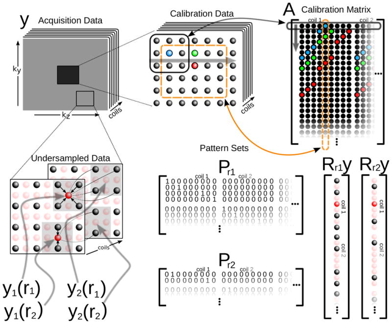
Data organization, indexing and operators that are used in the paper. Top: The calibration matrix A is constructed by sliding a window through the calibration data. The rows of A are overlapping k-space blocks from calibration data. Bottom-left: The indexing used to represent samples in k-space. Bottom-right: Applying Rr extracts a block in k-space and reorders it as a vector. Bottom-middle: Pattern set matrices associated with the k-space positions on the right. Applying PrRry extracts only acquired data from a block in k-space around position r.
| (4) |
where are data from the ith coil inside the AC region (orange square in the Fig. 1). In practice, kernels which solve this set of equations approximately are computed by solving a regularized least-squares problem [4, 16, 17].
By construction, one of the columns of A is . This is illustrated in Figure 1 where the area in the calibration marked by dashed orange square is used to construct the 5th column of A. We can write this as where ei is a vector with ‘1’ in the appropriate position that chooses the ith coil data, and ‘0’ elsewhere. Rewriting Equation 4, we get,
| (5) |
This means that are null-space vectors of the calibration matrix. The existence of a null-space implies redundancy in A and hence correlations between blocks of k-space, which can be used to synthesize missing samples. However are very specific null-space vectors which may represent only part of the redundant information. For this reason, we turn to characterize the null space directly.
Calibration Matrix and Null-Space Reconstruction
A very useful way to analyze the calibration matrix is to compute its singular value decomposition (SVD):
| (6) |
The columns of the V matrix in the SVD are a basis for the rows of A, and therefore basis for all the overlapping blocks in the calibration data. We can separate V into V⊥ which spans the null space of A and V‖ which spans its row-space. This is demonstrated well in Figure 2 using data obtained with an eight-channel head coil. The underlying information that we learn from the decomposition of the calibration data is that it lies in the subspace spanned by V‖ and not by V⊥. This information can then be used in the reconstruction to extrapolate unacquired measurements as this relation should be true for all the blocks in k-space and not just for the AC lines.
Figure 2.
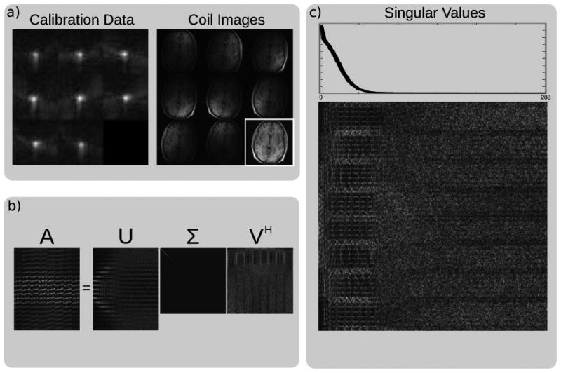
Singular value decomposition (SVD) of the calibration matrix. a) Magnitude of the calibration data in k-space and images from an eight-channel head coil. b) Magnitude of the SVD decomposition. The singular values are ordered by magnitude and appear on the diagonal of Σ. c) A zoomed view of the V matrix of the SVD and a plot of the singular vectors show that the calibration matrix has a null space. The k-space signal has support in V‖ and none in V⊥.
Given an undersampled k-space grid, each k-space block of the reconstruction x must satisfy two constraints,
| (7a) |
| (7b) |
The first is consistency with the calibration and the second is consistency with the data acquisition. Interpreting the (formally overdetermined) set of null-space constraints in the least-squares sense yields the normal equations
| (8) |
In the following, periodic boundary conditions are assumed, because they simplify the discussion considerably. Although this assumption is often implicitely used in MRI, it should be noted that it introduces minor numerical errors, which could be avoided by a rigorous derivation [18]. Assuming this, the equation can be transformed further to
| (9) |
where M represents and equals the number of samples in each patch of k-space data selected by Rr. This result can also be obtained by multiplying the first equation in 7a with from the left and summing over r. Because an operation of the form computes the correlation with each kernel in V‖ when performed for all r, it can be expressed as a set of convolutions.
This also applies to its adjoint and the symmetric product . Thus, by construction, 𝒲 is a convolution with a matrix-valued kernel where the matrix operates on the channel dimension. While the operations and are projections operating on patches, the operation 𝒲 is an average of projections and therefore Hermitian and positive semi-definite with eigenvalues smaller or equal to one.
Rewriting the first constraint in matrix form and merging all identical equations of the second constraint yields
| (10a) |
| (10b) |
where 𝒫 is a mask selecting only the acquired samples out of a full grid and results from merging the overlapping PrRr for all patches. The constraints can be enforced iteratively as in SPIRiT, which is different only in the operator 𝒲. This leads to a null-space reconstruction [13], which was independently developed by Zhang et. al., and reported in [19]. We extend these notions further and develop a new computationally efficient approach in which the connection to SENSE-based methods is made.
Sensitivity Maps as an Eigenvalue Problem
The null-space method (Eqs. 10) computes a solution in the null space of 𝒲 – I, while SENSE computes a solution in the subspace spanned by the coil sensitivities (Eq. 2). This suggests that these subspaces can be explicitly identified.
The solution x must satisfy 𝒲x = x, therefore, by definition, x belongs to a subspace spanned by the eigenvectors of 𝒲 corresponding to the eigenvalue ‘1’. If we write x in terms of the k-space of the original image weighted by the coil sensitivities, we get
| (11) |
where S = [S1S2 … SN]T is a vector of stacked coil sensitivities. Assuming that this is indeed a solution of Equations 10, we get
| (12) |
Applying the inverse Fourier transform on both sides of the equation, it follows that the vector of coil images is an eigenvector of ℱ−1𝒲ℱ for the eigenvalue ‘1’:
| (13) |
If we perform a direct eigenvalue decomposition of 𝒲, we should be able to find the sensitivities explicitly. Because the operator 𝒲 is a positive semi-definite matrix-valued convolution, it decouples into point-wise positive semi-definite matrix operations in the image domain:
| (14) |
The eigenvalue decomposition of the operator 𝒲 is simplified to solving a much smaller eigenvalue decomposition of 𝒢q for each position q in images space. The steps of one possible procedure for the computation of 𝒢q from the K kernels in V‖ are illustrated in Figure 3. Defining as the sensitivities at spatial position q and m(q) as the magnetization at this position, Equation 13 is reduced to
Figure 3.
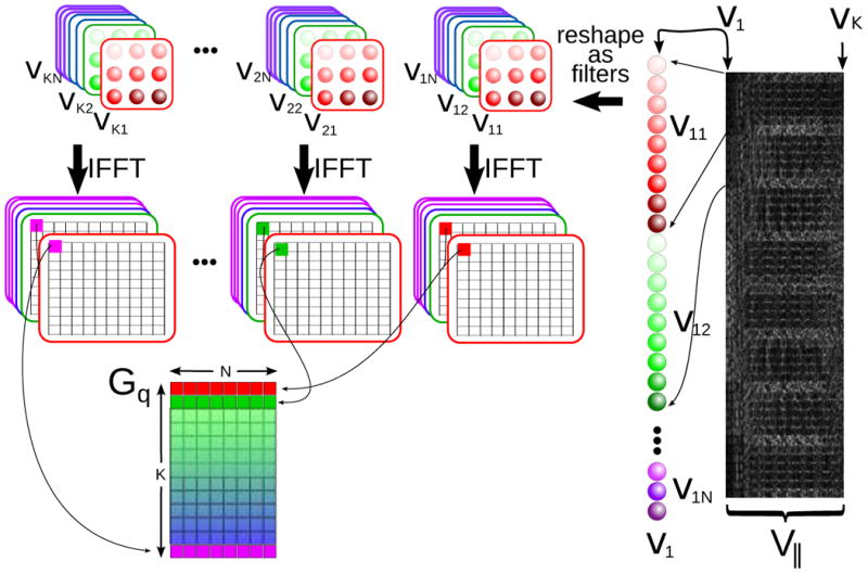
The construction of the 𝒢q matrices in Equation [14] is an efficient way to calculate the eigenvalues and vectors of 𝒲. Each basis vector in V‖ is reshaped (and flipped) into a convolution kernel in k-space. The convolutions can be efficiently implemented as multiplications in image space, resulting in separable K × N matrix multiplications Gq for each image-space position, where K is the number of kernels in V‖ (the rank of the calibration matrix A). Then .
| (15) |
At positions where m(q) is non-zero, this yields a condition for the sensitivities:
| (16) |
Thus, the explicit sensitivity maps can be found by an eigenvalue decomposition of all 𝒢q's choosing only the eigenvectors corresponding to eigenvalue ‘=1’. This is shown in Figure 4 for data from an eight-channel head coil. At locations where no eigenvalue ‘=1’ is found, the sensitivities are set to zero. These position correspond to locations without signal. The eigenvectors are defined only up to multiplication with an arbitrary complex number. For this reason, the norm of the eigenvectors at each location are normalized to one and one arbitrary chosen channel is used as a reference with zero phase [20].
Figure 4.
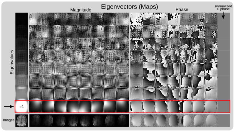
Explicit sensitivity maps from autocalibration data using eigenvalue decomposition: The figure shows the eigenvalues and eigenvectors of all 𝒢q in a map. 𝒢q has been computed as the Fourier transform of the reconstruction operator 𝒲 for data from an eight-channel head-coil using a 24 × 24 k-space calibration region and 6 × 6 kernel size. Left: Eigenvalues sorted in increasing magnitude from top to bottom. Eigenvalues ‘=1’ appear in positions where there is signal in the image. Right: Magnitude and phase of the eigenvector maps for each eigenvalue at all spatial positions. As expected, eigenvectors corresponding to eigenvalues ‘=1’ appear to be sensitivity maps. The magnitude and phase of the sensitivities follows closely the magnitude and phase of the individual coil images (bottom row). The eigenvectors are defined only up to multiplication with an arbitrary complex number. For this reason, the norm of the eigenvectors at each location are normalized to one and the 8th channel is used as a reference with zero phase.
In the ideal case, there is only a single eigenvector to the eigenvalue ‘1’ at each location and all other eigenvalues are ≪ 1. Then the solution for Equation 16 is equivalent to the projection onto the subspace spanned by the coil sensitivities (Eq. 2).
ESPIRiT: Implementation Using Soft SENSE
After computation of a single set of sensitivities, a standard SENSE reconstruction can be performed. In some cases errors in the acquisition lead to the appearance of multiple eigenvectors to eigenvalue ‘=1’ or additional eigenvalues smaller than one, indicating signal components which cannot be explained in terms of the strict SENSE model. Then, 𝒢q has the following form:
| (17) |
Here, Mq is usually one or two and all λj are often close to one. This motivates an extension of the reconstruction process: Instead of using a single set of sensitivity maps, Equation 1 is extended to a “soft” SENSE reconstruction, which uses a relaxed model of the signal based on multiple (M) image components mj and multiple sets of maps Sj:
| (18) |
A least-squares solution of this equation then yields several images (image components) mj at once.
In most applications the first component can be used as the reconstruction, while the other components represent errors which only have to be taken into account during reconstruction to avoid artifacts. If the other components present image content and can not be discarded, it might be necessary to do a magnitude combination to avoid signal loss due to phase cancellation. A third possibility is to compute the individual coil images according to and then combine the coil images mi in a post-processing step similar to GRAPPA. The first and last option can also be used for applications using phase information in the same way as SENSE and GRAPPA respectively.
As mentioned above, the reconstruction can be extended to integrate various regularization terms Q by formulating it as the optimization of a functional
| (19) |
For example, using the ℓ1-norm with a sparsity (e.g. wavelet) transform Ψ in yields ℓ1-ESPIRiT, which is usefull for a compressed sensing reconstruction of randomly undersampled data, similar to ℓ1-SPIRiT [4, 21].
Methods
In the spirit of reproducible research, we provide source code with examples for the proposed algorithm. It can be downloaded from: http://www.eecs.berkeley.edu/∼mlustig/Software.html
Fully-sampled data of the human brain was acquired on a 1.5 T scanner (GE, Waukesha, WI) using an eight-channel head coil for multiple subjects. Two data sets have been acquired with inversion-recovery prepared 3D RF-spoiled gradient-echo sequence (TR/TE = 12.2/5.2 ms and TR/TE = 9.7/4.1 ms, TI = 450 ms, FA = 20°, BW = 15 kHz, matrix size: 256 × 180 × 230 and 200 × 200 × 200, resolution: 1 mm isotropic) and one data set with a 2D spin-echo sequence (TR/TE = 550/14 ms, FA = 90°, BW = 19 kHz, matrix size: 320 × 168, slices: 6, slice thickness: 3 mm) using a reduced FOV of 200 mm × 150 mm, which was smaller than the head of the subject in phase-encoding direction (lateral).
The 3D data has been Fourier transformed along the readout direction and all further processing has been done for 2D k-space data of selected sections. The computation of the eigenvalue and eigenvector maps and the ESPIRiT reconstruction have been implemented in MatLab (MathWorks, Natick, MA) and in the C programming language using the FFTW [22] (http://www.fftw.org) and ACML (http://www.amd.com/acml, AMD, Sunnyvale, CA) libraries. For the computation of the eigendecomposition of 𝒢q, a version using orthogonal iteration has been implemented, which allows the efficient computation of the eigenvectors of only the largest eigenvalues. The number of iterations was set to 30.
The basic assumptions of the present work have been confirmed by computing the SVD of the calibration matrix and computing all eigenvalue and eigenvector maps for a single section of a 3D RF-spoiled gradient-echo data set using a calibration region of size 24 × 24 and a kernel size of 6 × 6.
In the following experiments, the quality of the computed sensitivity maps has been evaluated in different ways. If not mentioned otherwise, a calibration region of size 20 × 20 and kernel size of 5 × 5 has been used. In this work, the size of the null space has been estimated by setting a cut-off relative to the maximum singular value. The effect of this parameter has been evaluated for different values for k = 1 ⋯5 by computing eigenvalue maps and computing sensitivity maps corresponding to the largest eigenvalue. For these sensitivity maps, it has been tested how well fully-sampled data can be reproduced. In detail, fully-sampled coil images mj are projected onto the subspace spanned by the maps (see Eq. 2) and then the original images mj are subtracted to obtain the projection onto its orthogonal complement:
| (20) |
This shows the part of the images mj which is in the null space as approximated by the maps. Only noise should remain and any residual signal indicates imperfections of the sensitivities. For better visualization, the residual images for all channels have been combined by computing the point-wise root of the sum of absolute squares.
For the same data, the reconstruction quality of ESPIRiT has been compared with other autocalibrating parallel imaging algorithms. The following algorithms have been used: SENSE reconstruction using sensitivities estimated from the fully sampled k-space center according to [9], nonlinear inverse reconstruction (NLINV) [11], and GRAPPA [3] as described in the present work. The null space has been determined using and sensitivity maps have then been computed at all locations with eigenvalues larger than a threshold 0.9 and set to zero elsewhere. Reconstructions have been performed for a single section of a 3D data set orthogonal to the readout direction, which has retrospectively been undersampled along both phase-encoding direction by factors 3 × 2 and 2 × 2. GRAPPA kernels have been regularized by Tikhonov regularization with 3 × 10⁻⁴ relative to the 2-norm of AH A. SENSE and ESPRiT reconstructions have been regularized with 0.001 (using normalized sensitivities and Fourier transform), while NLINV was used with nine Newton steps.
Again using the same parameters, the quality of the calibration of different methods has been compared by computing how well fully-sampled data can be reproduced (as described above). For GRAPPA, a combined reconstruction kernel has been computed for a regular undersampling of 3 × 2 and used in place of in Equation 20. It should be noted that the computation of all necessary GRAPPA kernels depends on the sampling scheme, and the combination into a single convolution kernel is possible for regular sampling on a grid. Then, all kernels can be applied everywhere using a convolution, because the sampling pattern matched to a patch at a shifted location between the intended grid positions yields PrRr = 0.
To study the effect of different noise level on the calibration Gaussian white noise has been added to k-space to create data with 10× and 20× the noise level of the original acquisition. Using the same parameters as above, ESPIRiT calibration has been performed and the accuracy of the obtained sensitivity maps has been evaluated by projecting fully-sampled coil images mj of the original data onto the subspace spanned by the maps (see Eq. 2). In addition, images have been reconstructed for all noise levels for undersampling in both phase-encoding directions by 2 × 2 using ESPIRiT and GRAPPA.
That ESPIRiT has similar properties as GRAPPA is demonstrated with examples where the FOV is smaller than the object. Eigenvalue and eigenvector maps have been computed for a data set with full FOV, with reduced FOV in one dimension, and with reduced FOV in two dimensions. The ability to reconstruct proper images in this case by using multiple maps is demonstrated for spin-echo data, which has been undersampled by a factor of two in the phase-encoding (lateral) direction, and compared with other reconstruction algorithms. Here, a lower threshold of 0.8 has been used for calculation of the sensitivity maps to avoid truncation artifacts.
Finally, the behavior for other kinds of data corruption has been investigated with two examples. The first example used single-shot fly-back EPI (TE = 78.4 ms, ΔTE = 1.504 ms, BW = 125 kHz, matrix size: 128 × 48, FOV: 35 mm, slice thickness: 4 mm) of a human brain without fat suppression. Maps and corresponding images from an ESPIRiT reconstruction have been computed (calibration region: 24 × 24, kernel size: 6 × 6, , threshold: 0.9). The second example used 3D fast spin-echo MRI (TR/TE = 1,600/20.8 ms, 37 echos, BW = 62.5 kHz, matrix size: 320 × 288 × 236, resolution: 0.5 mm × 0.5 mm × 0.6 mm) of a human knee, which has been accelerated by a factor of 8.4 using variable-density Poisson-disc sampling [23]. Here, 3D sensitivity maps have been computed (calibration region: 243, kernel size: 63, , threshold: 0.9) for an eight-channel coil compressed to six virtual channels [24]. Each section along the readout direction has been reconstructed with a compressed-sensing ℓ1-ESPIRiT reconstruction with wavelet regularization. Volumes corresponding to the different maps have then been combined as described before to obtain a single volume for comparison with a similar ℓ1-SPIRiT [4, 21] reconstruction.
Results
The basic assumptions of the present work have been validated by computing the singular value decomposition of a calibration matrix constructed from experimental eight-channel data (Fig. 2). The data used to construct A was of size 24 × 24 × 8, and the kernel size (window size) was 6 × 6. These correspond to A being a [(24 − 6 + 1)2 × (6*6*8)] = [361 × 288] matrix. The figure shows the calibration data in k-space and the magnitude of the associated A, U, Σ and V matrices. It confirms that A indeed has a null space, which relates to the fact that the rows of A are correlated. That sensitivity maps can be estimated using the procedure outlined in the present work is demonstrated in Figure 4. It shows eigenvalue and eigenvector maps, which have been obtained by a point-wise eigendecomposition of the operator 𝒲. There exists an eigenvalue ‘=1’ everywhere in the area of support of the image, and the corresponding eigenvector has the structure of normalized coil sensitivities. The last row shows the corresponding individual coil images for comparison.
Figure 5 shows eigenvalue maps computed using a row space V‖ with different size K, which has been estimated by a cut-off σcut-off relative to the largest singular value of the calibration matrix. Here and in the following, the calibration matrix of size [(20 − 5 + 1)2 × (5 * 5 * 8)] = [256 × 200] has been computed from a calibration region of size 20 × 20 × 8 and for a kernel size of 5 × 5. For the values with k = 1 … 5 the number of kernels in V‖ are K = 21, 33, 44, 57, 101, respectively, from a total of 200 kernels. For higher thresholds, the estimated V‖ gets smaller until parts of the signal gets incorrectly included into the null space V⊥. In this case, even the largest eigenvalue of 𝒢q becomes smaller than one inside the support of the image. For lower thresholds, the null space gets very small and does not fully capture all correlations in the data. In the extreme case, when there is no null space left, all eigenvalues are ‘=1’ (not shown). Both extremes lead to errors in the sensitivities, which is evident by visual inspection of the sensitivities and indicated by residual energy in the projection of fully-sampled coil images onto the null space as approximated by the maps using Equation 20. Very good sensitivities can be obtained for a large range of values between .
Figure 5.
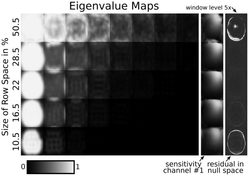
Eigenvalue maps computed when using a different number of kernels to estimate the row space V‖ of the calibration matrix A (rows). The percentages with respect to the total number of kernels are shown, corresponding to 101, 57, 44, 33, 21 kernels out of 200. The rightmost column shows a projection of fully-sampled coil images onto the null space as approximated by the sensitivities using Equation [20] (scaled by a factor 5 compared to the corresponding anatomical images in the following figures). If this projection contains residual energy in addition to noise, this indicates errors in the calibration.
Reconstructions using the estimated sensitivities are compared to other reconstruction algorithms for undersampling factors of 2 × 2 and 3 × 2 (see Fig. 6). For 2 × 2 undersampling, ESPIRiT and NLINV reconstruct artifact-free images, which have slightly better quality than the images reconstructed with SENSE and GRAPPA. For higher acceleration, all reconstructions start to deteriorate showing increased noise and aliasing artifacts (the trade-off is controlled by the regularization parameter). Under the experimental conditions chosen here, GRAPPA shows more severe artifacts and noise amplification compared to the other three algorithms, indicating errors in the calibration of the GRAPPA kernels. In contrast, the ESPIRiT algorithm, which uses sensitivities estimated from exactly the same calibration matrix as GRAPPA, allows a better reconstruction similar to the other SENSE-based algorithms. This is further confirmed by a direct evaluation of the quality of the maps. The last row of Figure 6 shows the projection of the coil images obtained from fully-sampled data onto the null space of different reconstruction methods. For NLINV and ESPIRiT the signal is almost completely removed and only noise remains, while for the other two algorithms some remaining signal indicates errors in the calibration.
Figure 6.
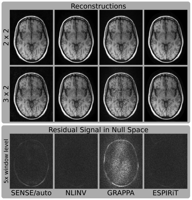
Images of a human brain. Fully-sampled data from an eight-channel coil has been retrospectively undersampled by factors of 2 × 2 and 3 × 2. Reconstruction has been performed using SENSE with autocalibration (SENSE/auto), nonlinear inversion (NLINV), GRAPPA, and ESPIRiT. The projection of fully-sampled individual coil images onto the null space has been computed for all methods and combined to a single image scaled by a factor of 5 (bottom row). For GRAPPA, the projection corresponds to a reconstruction operator corresponding to a regular 2 × 3 undersampling pattern. If the null space contains residual energy in addition to noise, this indicates errors in the calibration.
Data with different noise-level (orignal, 10×, 20×) has been used for calibration and reconstruction using ESPIRiT and GRAPPA (Fig. 7). The projection of the coil images of the original data onto the null space defined by ESPIRiT sensitivities shows only slightly increasing error even for a very high noise level. The images reconstructed from 2 × 2 undersampled data with the original noise level using ESPIRiT and GRAPPA are identical the images shown in Figure 6 and show better image quality for ESPIRiT than for GRAPPA, which is slightly compromised by aliasing artifacts. For higher noise levels, the images from both algorithms get disturbed by noise, although ESPIRiT is less affected than GRAPPA.
Figure 7.
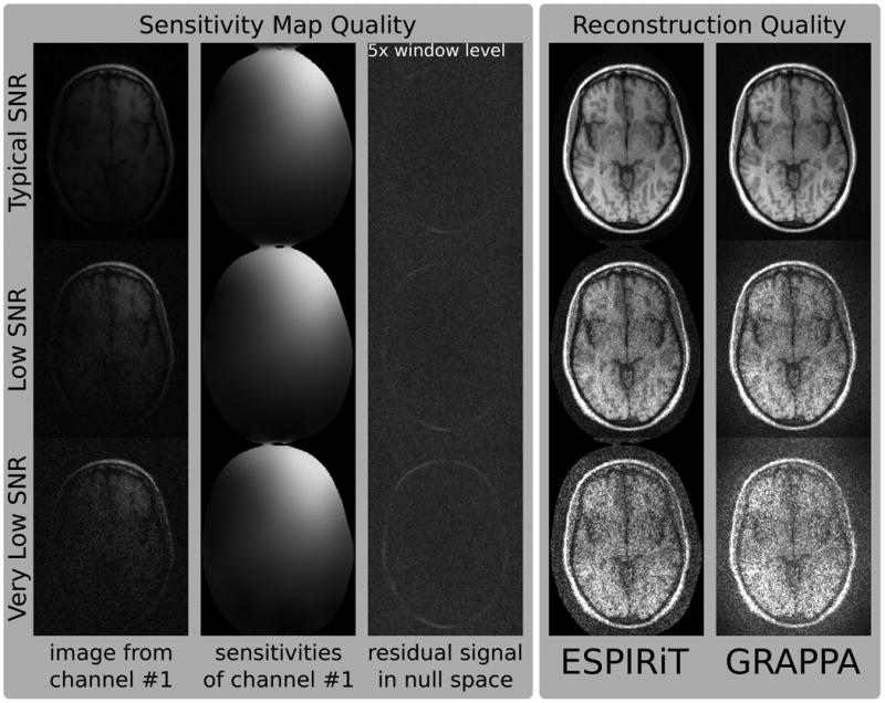
The effect of noise on the calibration of the sensitivity maps has been studied by adding noise to fully-sampled data (noise levels: 1×, 10×, 20×). 1st column: Fully-sampled images corresponding to the first channel for different noise levels. 2nd column: Sensitivity map of the first channel as estimated using the ESPIRiT calibration. 3rd column: The projection of the fully-sampled original data onto the nullspace defined by the sensitivities (scaled by a factor of 5). 4th and 5th column: Reconstruction results for ESPIRiT and GRAPPA for 2 × 2 undersampling.
In the following experiments, the FOV has been choosen to be smaller than the head of the subject. Figure 8 shows maps from a measurement where the FOV has been reduced in one and in two dimensions. Up to four eigenvectors for eigenvalue ‘=1’ appear in overlapping areas. This corresponds to the observation that a single smooth sensitivity map is not able to model the data correctly, but that this is possible using multiple maps. Figure 9 shows respective reconstructions from a two-fold undersampled scan. The methods assuming a single set of smooth sensitivity maps, i.e. SENSE with direct calibration and NLINV, are not able to recover correct coil sensitivities. The reconstructions show a severe artifact in the center of the image, which is absent for GRAPPA and ESPIRIT.
Figure 8.
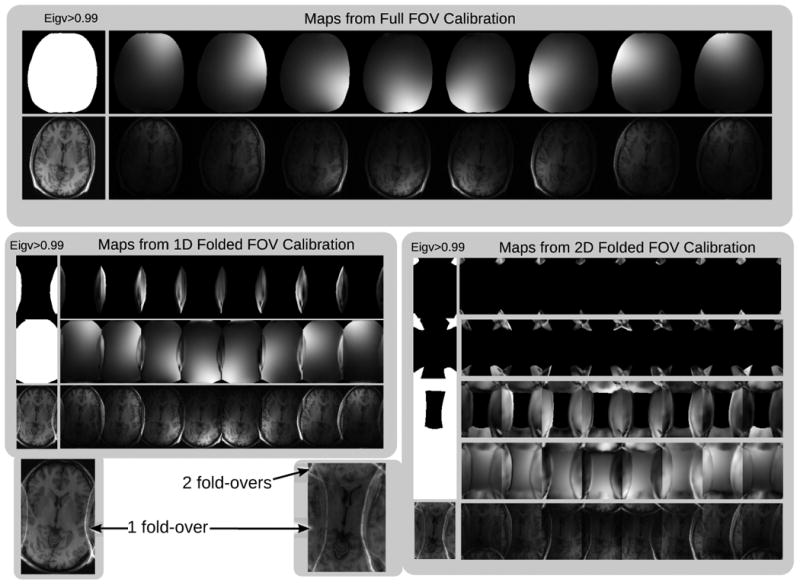
The effect of reduced FOV of the calibration lines. Top: When the supported FOV of the calibration covers the entire image, there is a single eigenvalue ‘=1’ at each spatial position and a single set of sensitivity maps. Bottom: When the the supported FOV of the calibration is smaller than the image, there are multiple eigenvalues ‘=1’ at positions that exhibit folding. For each eigenvalue ‘=1’ there is an associated set of sensitivity maps that is needed to faithfully represent the data. GRAPPA-like autocalibration methods implicitly use all the sensitivities with eigenvalues ‘=1’ and are not prone to the FOV limitation that is described in [14]. The eigenvalue approach is a tool to find these sensitivities explicitly. These sensitivities can be used in a SENSE-like ESPIRiT reconstruction that exhibits the same robustness to the calibration FOV as autocalibrating methods.
Figure 9.
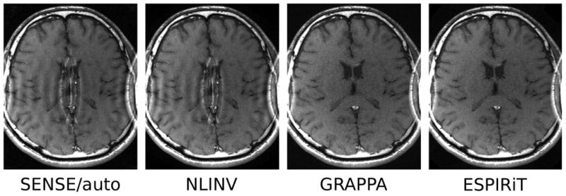
Reconstruction from two-fold undersamed data acquired with a FOV smaller than the object. In this case, a single set of sensitivity maps on the restricted FOV cannot represent the signal correctly. Direct calibration and nonlinear inversion cannot recover the sensitivities, and the corresponing reconstructed images have a severe artifact in the center of the image (SENSE/auto and NLINV). GRAPPA and ESPIRiT are able to reconstruct the center of the image correctly.
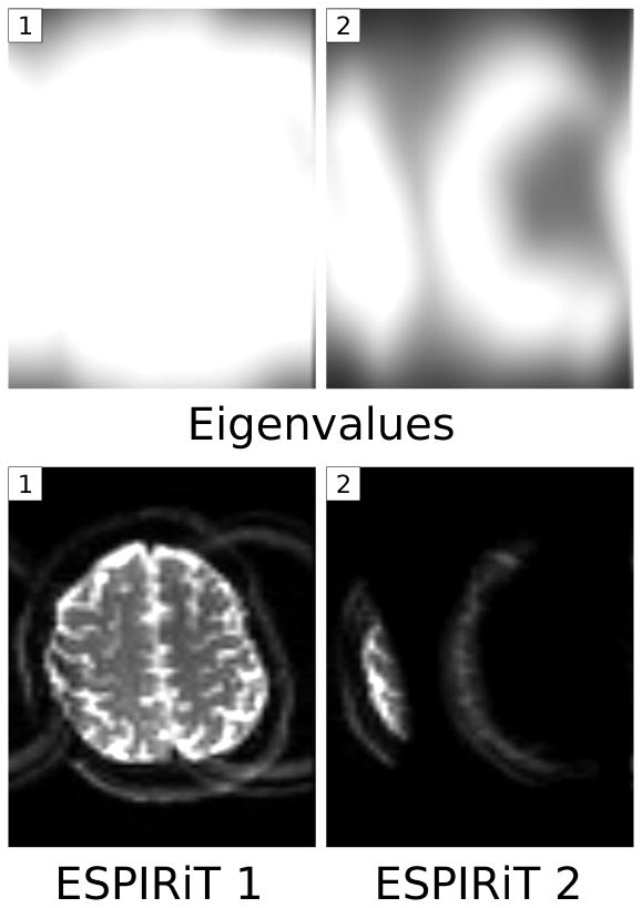
Multiple eigenvalues can also appear for other reasons. Figure 10 shows images of a highly-accelerated 3D fast spin-echo acquisition of a human knee presumably corrupted by motion. An additional eigenvalue close to one appears in the parts of the image, which are affected by motion, and the corresponding ESPIRiT reconstructions yield multiple image components. A comparison between ℓ1-ESPIRiT using only the first and using two maps shows that the use of additional maps can be beneficial. Restricting the reconstruction to use only one map as in SENSE causes a loss of signal, while the use of two maps yields image quality similar to ℓ1-SPIRiT. Figure 11 (supplementary material) shows eigenvalue maps for a single-shot EPI scan of a human brain without fat suppression. Here, an additional eigenvalue close to one appears in the parts of the image, which are affected by the shifted fat signal. The corresponding ESPIRiT reconstructions yield multiple images which reflect the different signal components.
Figure 10.
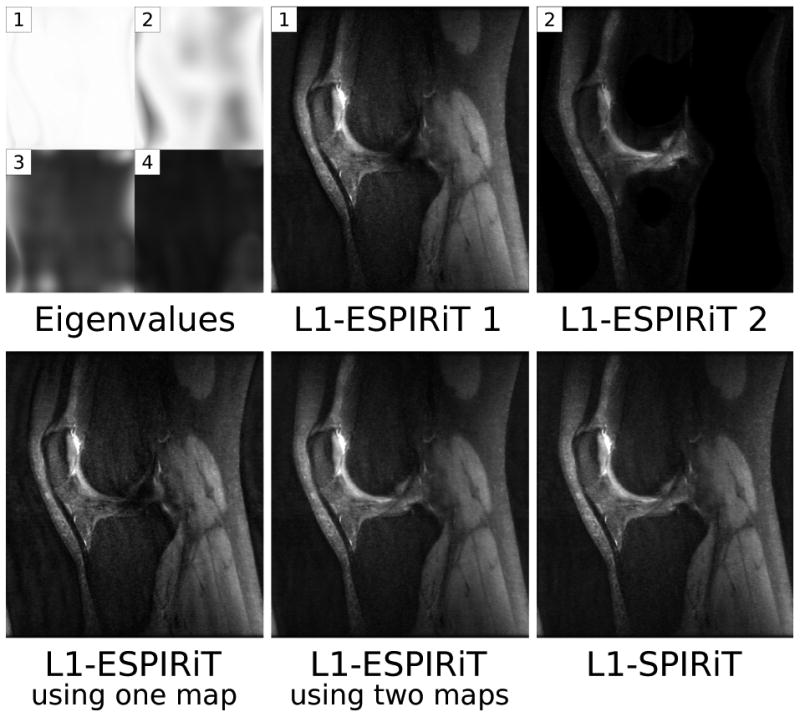
A single sagittal section from a motion-corrupted 3D scan of a human knee (readout direction: superior-inferior). Additional eigenvalues appear and the reconstruction with two sets of sensitivity maps yields two images (top). When restricting the ℓ1-ESPIRiT reconstruction to use only one set of maps, the signal corresponding to the second component is lost and additional artifacts appear. The combined image from ℓ1-ESPIRiT using two maps and the image reconstructed with ℓ1-SPIRIT do not suffer from this problem (bottom).
Figure 11.
Single-shot EPI of the human brain without fat suppression. The signals of water and shifted fat are not compatible with a single sensitivity map, and the maps of the two highest eigenvalues show that an additional eigenvalue appears in affected locations (top). An ESPIRiT reconstruction using two sets of sensitivity maps yields two separate images (bottom).
Discussion
Null Space of the Calibration Matrix
Doing a coil-by-coil calibration in k-space involves building the calibration matrix A. The linear dependence between the samples causes A to have a null space. Values in the row space of A correspond to the underlying signal, whereas those in the null space are not consistent and correspond to noise. This idea to analyze a correlation matrix to identify signal and noise subspaces has been known for a long time in frequency estimation [25, 26, 27]. Similar ideas have been used multichannel blind deconvolution [28, 29] and exploited for autocalibrated parallel MRI [30, 31]. The idea is also used in recent work about calibrationless parallel MRI reconstruction using low-rank matrix completion [32].
The vectors that span the null space can be used to synthesize missing samples. This leads to a null-space reconstruction [19, 13], which can be understood as an improved version of the SPIRiT algorithm [4]. In the null-space reconstruction, the reconstruction operator is constructed directly from the SVD of the calibration matrix, and is guaranteed to only pass components in row space and none in null space, which is not necessarily true for the original SPIRiT operator.
Properties of GRAPPA
As shown in the present work, GRAPPA kernels are also related to null-space vectors of the calibration matrix. This insight leads to a better understanding of GRAPPA, whose properties have sometimes been described as paradoxical [33, 34]. GRAPPA kernels have a specific structure to allow reconstruction in a single step: they only have entries where samples have been acquired and are required to have a one in the center. Due to these restrictions, the least-squares solution often only approximates the null-space constraint and this approximation becomes worse with higher acceleration as fewer and fewer entries are allowed and GRAPPA becomes less and less accurate. The examples shown in the present work use a relatively small kernel size, which makes them more susceptible to this effect. SPiRiT and null-space kernels do not depend on the sampling pattern and make use of all but one samples in each patch, allowing a more accurate approximation of the null-space constraint.
GRAPPA kernels are usually not uniquely defined by the null-space constraint. This makes it possible to choose the one with the smallest norm using regularization, which avoids noise amplification during the reconstruction. A paradoxical effect related to this is that the quality of a GRAPPA reconstruction can improve with increasing noise in the calibration area, which has been empirically described in [34]. The existence of a null space of the calibration matrix implies that its condition number is infinite in the ideal noise-less case and becomes finite only due to noise (or explicit regularization). Another property of GRAPPA which has remained somewhat mysterious is the ability to reconstruct images even when the FOV becomes smaller than the object [14, 33]. In this case even the calibration data itself becomes undersampled. As shown here for null-space kernels, this is related to the appearance of multiple eigenvectors to the eigenvalue one in the reconstruction operator.
Computation of Sensitivity Maps
This work links GRAPPA, SPIRiT, and the null-space method to SENSE-based reconstruction techniques which make explicit use of coil sensitivities. The sensitivities can be calculated from an eigendecomposition of the reconstruction operator, which can be performed efficiently in the image domain. This local computation of the sensitivities has some similarity to a previously published method for the estimation of the sensitivities from a local correlation matrix in image space [35, 20] and could also be thought of as a generalization of the subspace-based method presented in [36]. Using these sensitivities for image reconstruction offers all advantages of SENSE, i.e. linear scaling with the number of receive channels with respect to computational demand, optimal reconstruction quality, straightforward extension to non-Cartesian sampling, and integration of various types of regularization techniques.
With a sufficiently large calibration area, the technique decribed in the present work allows the estimation of the sensitivities with very high precision, as demonstrated by direct evaluation of their accuray and by comparison with other methods. Notably, this is possible even though the kernels are usually too small to fully capture all correlations in k-space. Iterative enforcement of the constraints as in SPIRiT at all positions in k-space leads to additional consistency conditions, which are not visible in a small patch of k-space. This is similar to how a repeated application of a filter with small support can achieve a sharper transition from stop to pass band than what is possible with a single application. Computing the eigenvector to the eigenvalue ‘=1’ of the reconstruction directly extracts a consistent subspace, which then describes also correlations in k-space which might reach further than the size of the kernel.
Reconstruction with Multiple Maps
Multiple eigenvectors to the eigenvalue one appear when the data does not conform to the SENSE model. By extending a SENSE reconstruction to use multiple maps, these additional signal components can be taken into account. For example, it is possible to reconstruct images from under-sampled data without a central aliasing artifact when using a small FOV, which is possible with GRAPPA and SPIRiT, but not with basic SENSE or NLINV. It should be noted that NLINV can also recover a correct image in this situation, when explicitely using an extended FOV in the reconstruction [18]. Other errors might also lead to the occurrence of additional eigenvalues, as long as the calibration region is affected. For example, in the case of a shifted fat ghost in single-shot EPI the appearance of an additional map corresponds to the fact that the fat signal is compatible with shifted coil sensitivities [37, 38]. Because the two components do not correspond to water and fat, but to an arbitrary mixture, a separation or a removal of the fat signal is not directly possible. Nevertheless, the use of two maps could allow a parallel MRI reconstruction, which would have errors related to the fat signal when using only one map. For other errors additional maps might also allow an improved reconstruction, such as in the example of with motion corruption, although this depends on the exact nature of the corruption and can not always be expected. While noise behavior using a single set of maps is identical to SENSE-based methods, this changes when multiple maps are used. In this case, g-factor maps can be computed using a straightforward extension of the formula given by Pruessmann et al. [2] for periodic sampling and with Monte-Carlo methods in the general case.
Computation Time
Using a multi-threaded implementation on two CPUs with six cores, calibration for a single 2D slice and iterative reconstruction using two maps each took less than one second for all presented examples. Calibration and compressed-sensing parallel-imaging reconstruction of the complete 3D knee data set took about 1:30 minutes and 4:30 minutes, respectively. With an implementation using similar to [21] using four CPUs, the 3D reconstruction can be performed in 2 minutes. Because the point-wise eigendecomposition is parallelizable, a similar speed-up is expected from a GPU implementation of the calibration, which is already in development.
Conclusions
In this paper, the gap between the two main approaches to parallel MRI has finally been bridged. We have shown that all parallel imaging methods restrict the solution to a subspace spanned by the coil-sensitivities. Based on this observation, properties of methods such as GRAPPA and SPIRiT can be analyzed and better understood. In addition, a new hybrid reconstruction method has been presented, which combines the advantages from both approaches. While other related methods which operate in k-space such as nullspace method (PRUNO) may achieve comparable image quality, they don't offer the flexibility and efficiency of the proposed image-domain method. Nevertheless, more work will necessary to define the most optimal method for a given application.
Supplementary Material
Acknowledgments
This work was supported by NIH grants P4IRR09784, R0IEB009690, American Heart Association I2BGIA9660006, UC Discovery Grant 193037, and GE Healthcare.
Footnotes
Presented in part at the 19th Annual Meeting of ISMRM, Montreal, Canada, 2011.
References
- 1.Ra JB, Rim CY. Fast imaging using subencoding data sets from multiple detectors. Magn Reson Med. 1993;30:142–145. doi: 10.1002/mrm.1910300123. [DOI] [PubMed] [Google Scholar]
- 2.Pruessmann KP, Weiger M, Scheidegger MB, Boesiger P. SENSE: Sensitivity encoding for fast MRI. Magn Reson Med. 1999;42:952–962. [PubMed] [Google Scholar]
- 3.Griswold MA, Jakob PM, Heidemann RM, Nittka M, Jellus V, Wang J, Kiefer B, Haase A. Generalized autocalibrating partially parallel acquisitions (GRAPPA) Magn Reson Med. 2002;47:1202–1210. doi: 10.1002/mrm.10171. [DOI] [PubMed] [Google Scholar]
- 4.Lustig M, Pauly JM. SPIRIT: Iterative self-consistent parallel imaging reconstruction from arbitrary k-space. Magn Reson Med. 2010;64:457–471. doi: 10.1002/mrm.22428. [DOI] [PMC free article] [PubMed] [Google Scholar]
- 5.Pruessmann KP, Weiger M, Börnert P, Boesiger P. Advances in sensitivity encoding with arbitrary k-space trajectories. Magn Reson Med. 2001;46:638–651. doi: 10.1002/mrm.1241. [DOI] [PubMed] [Google Scholar]
- 6.Raj A, Singh G, Zabih R, Kressler B, Wang Y, Schuff N, Weiner M. Bayesian parallel imaging with edge-preserving priors. Magn Reson Med. 2007;57:8–21. doi: 10.1002/mrm.21012. [DOI] [PMC free article] [PubMed] [Google Scholar]
- 7.Block KT, Uecker M, Frahm J. Undersampled radial MRI with multiple coils. Iterative image reconstruction using a total variation constraint. Magn Reson Med. 2007;57:1086–1098. doi: 10.1002/mrm.21236. [DOI] [PubMed] [Google Scholar]
- 8.Lustig M, Donoho DL, Pauly JM. Sparse MRI: The application of compressed sensing for rapid MR imaging. Magn Reson Med. 2007;58:1182–1195. doi: 10.1002/mrm.21391. [DOI] [PubMed] [Google Scholar]
- 9.McKenzie CA, Yeh EN, Ohliger MA, Price MD, Sodickson DK. Self-calibrating parallel imaging with automatic coil sensitivity extraction. Magn Reson Med. 2002;47:529–538. doi: 10.1002/mrm.10087. [DOI] [PubMed] [Google Scholar]
- 10.Ying L, Sheng J. Joint image reconstruction and sensitivity estimation in SENSE (JSENSE) Magn Reson Med. 2007;57:1196–1202. doi: 10.1002/mrm.21245. [DOI] [PubMed] [Google Scholar]
- 11.Uecker M, Hohage T, Block KT, Frahm J. Image reconstruction by regularized nonlinear inversion – Joint estimation of coil sensitivities and image content. Magn Reson Med. 2008;60:674–682. doi: 10.1002/mrm.21691. [DOI] [PubMed] [Google Scholar]
- 12.Lai P, Lustig M, Brau AC, Vasanawala S, Beatty PJ, Alley M. Efficient L1SPIRiT reconstruction (ESPIRiT) for highly accelerated 3d volumetric MRI with parallel imaging and compressed sensing. Proceedings of the 18th Annual Meeting of the ISMRM; Stockholm. 2010. p. 345. [Google Scholar]
- 13.Lustig M, Lai P, Murphy M, Vasanawala SS, Elad M, Zhang J, Pauly JM. An eigen-vector approach to autocalibrating parallel MRI, where SENSE meets GRAPPA. Proceedings of the 19th Annual Meeting of the ISMRM; Montreal. 2011. p. 479. [Google Scholar]
- 14.Griswold MA, Kannengiesser S, Heidemann RM, Wang J, Jakob PM. Field-of-view limitations in parallel imaging. Magn Reson Med. 2004;52:1118–1126. doi: 10.1002/mrm.20249. [DOI] [PubMed] [Google Scholar]
- 15.Samsonov AA, Kholmovski EG, Parker DL, Johnson CR. POCSENSE: POCS-based reconstruction for sensitivity encoded magnetic resonance imaging. Magn Reson Med. 2004;52:1397–1406. doi: 10.1002/mrm.20285. [DOI] [PubMed] [Google Scholar]
- 16.Qu P, Wang C, Shen GX. Discrepancy-based adaptive regularization for GRAPPA reconstruction. J Magn Reson Imaging. 2006;24:248–255. doi: 10.1002/jmri.20620. [DOI] [PubMed] [Google Scholar]
- 17.Liu W, Tang X, Ma Y, Gao JH. Improved parallel MR imaging using a coefficient penalized regularization for GRAPPA reconstruction. Magn Reson Med. 2013;69:1109–1114. doi: 10.1002/mrm.24344. [DOI] [PubMed] [Google Scholar]
- 18.Uecker M. PhD thesis. Georg-August-Universität; Göttingen: 2009. Nonlinear Reconstruction Methods for Parallel Magnetic Resonance Imaging. [Google Scholar]
- 19.Zhang J, Liu C, Moseley ME. Parallel reconstruction using null operations. Magn Reson Med. 2011;66:1241–1253. doi: 10.1002/mrm.22899. [DOI] [PMC free article] [PubMed] [Google Scholar]
- 20.Griswold M, Walsh D, Heidemann R, Haase A, Jakob P. The use of an adaptive reconstruction for array coil sensitivity mapping and intensity normalization. Proceedings of the 10th Annual Meeting of the ISMRM; Honolulu, Hawaii. 2002. p. 2410. [Google Scholar]
- 21.Murphy M, Alley M, Demmel J, Keutzer K, Vasanawala S, Lustig M. Fast ℓ1-SPIRiT compressed sensing parallel imaging MRI: Scalable parallel implementation and clinically feasible runtime. IEEE Trans Med Imaging. 2012;31:1250–1262. doi: 10.1109/TMI.2012.2188039. [DOI] [PMC free article] [PubMed] [Google Scholar]
- 22.Frigo M, Johnson SG. The design and implementation of FFTW3. Proc IEEE. 2005;93:216–231. [Google Scholar]
- 23.Vasanawala SS, Murphy MJ, Alley MT, Lai P, Keutzer K, Pauly JM, Lustig M. I S Biomed Imaging. Chicago: 2011. Practical parallel imaging compressed sensing MRI: Summary of two years of experience in accelerating body MRI of pediatric patients; pp. 1039–1043. [DOI] [PMC free article] [PubMed] [Google Scholar]
- 24.Zhang T, Pauly JM, Vasanawala SS, Lustig M. Coil compression for accelerated imaging with cartesian sampling. Magn Reson Med. 2012 doi: 10.1002/mrm.24267. [DOI] [PMC free article] [PubMed] [Google Scholar]
- 25.Pisarenko VF. The retrieval of harmonics from a covariance function. Geophys J Roy Astr S. 1973;33:347–366. [Google Scholar]
- 26.Schmidt RO. Multiple emitter location and signal parameter estimation. IEEE Trans Antennas Propag. 1986;34:276–280. [Google Scholar]
- 27.Roy R, Kailath T. ESPRIT - Estimation of signal parameters via rotational invariance techniques. IEEE Trans Acoust Speech Signal Process. 1989;37:984–995. [Google Scholar]
- 28.Harikumar G, Bresler Y. Perfect blind restoration of images blurred by multiple filters: Theory and efficient algorithms. IEEE Trans Image Process. 1999;8:202–219. doi: 10.1109/83.743855. [DOI] [PubMed] [Google Scholar]
- 29.Sharif B, Bresler Y. Generic feasibility of perfect reconstruction with short FIR filters in multichannel systems. IEEE Trans Sig Proc. 2011;59:5814–5829. [Google Scholar]
- 30.She H, Chen RR, Liang D, Chang Y, Ying L. I S Biomed Imaging. Rotterdam: 2010. Image reconstruction from phased-array MRI data based on multichannel blind deconvolution; pp. 760–763. [DOI] [PubMed] [Google Scholar]
- 31.Sharif B, Bresler Y. I S Biomed Imaging. Chicago: 2011. Distortion-optimal self-calibrating parallel MRI by blind interpolation in subsampled filter banks; pp. 52–56. [DOI] [PMC free article] [PubMed] [Google Scholar]
- 32.Lustig M, Elad M, Pauly JM. Calibrationless parallel imaging reconstruction by structured low-rank matrix completion. Proceedings of the 18th Annual Meeting of the ISMRM; Stockholm. 2010. p. 2870. [Google Scholar]
- 33.Beatty PJ, Brau AC. Understanding the GRAPPA paradox. Proceedings of the 14th Annual Meeting of the ISMRM; Seattle. 2006. p. 2467. [Google Scholar]
- 34.Ding Y, Xue H, Chang T, Guetter C, Simonetti O. A quantitative study of Sodickson's paradox. Proceedings of the 20th Annual Meeting of the ISMRM; Melbourne. 2012. p. 3352. [Google Scholar]
- 35.Walsh DO, Gmitro AF, Marcellin MW. Adaptive reconstruction of phased array MR imagery. Magn Reson Med. 2000;43:682–690. doi: 10.1002/(sici)1522-2594(200005)43:5<682::aid-mrm10>3.0.co;2-g. [DOI] [PubMed] [Google Scholar]
- 36.Morrison RL, Jacob M, Do MN. I S Biomed Imaging. Washington: 2007. Multichannel estimation of coil sensitivities in parallel MRI; pp. 117–120. [Google Scholar]
- 37.Larkman DJ, Counsell S, Hajnal JV. Water and fat separation using standard SENSE processing. Proceedings of the 13th Annual Meeting of the ISMRM; Miami Beach. 2005. p. 505. [Google Scholar]
- 38.Uecker M, Lustig M. Making SENSE of chemical shift: Separating species in single-shot EPI using multiple coils. Proceedings of the 20th Annual Meeting of the ISMRM; Melbourne. 2012. p. 2490. [Google Scholar]
Associated Data
This section collects any data citations, data availability statements, or supplementary materials included in this article.


