Abstract
We propose an efficient methodology for comparing computational models of a perceptually discriminable quantity. Rather than comparing model responses to subjective responses on a set of pre-selected stimuli, the stimuli are computer-synthesized so as to optimally distinguish the models. Specifically, given two computational models that take a stimulus as an input and predict a perceptually discriminable quantity, we first synthesize a pair of stimuli that maximize/minimize the response of one model while holding the other fixed. We then repeat this procedure, but with the roles of the two models reversed. Subjective testing on pairs of such synthesized stimuli provides a strong indication of the relative strengths and weaknesses of the two models. Specifically, the model whose extremal stimulus pairs are easier for subjects to discriminate is the better model. Moreover, careful study of the synthesized stimuli may suggest potential ways to improve a model or to combine aspects of multiple models. We demonstrate the methodology for two example perceptual quantities: contrast and image quality.
Keywords: model comparison, maximum differentiation competition, perceptual discriminability, stimulus synthesis, contrast perception, image quality assessment
Introduction
Given two computational models for a perceptually discriminable quantity, how can we determine which is better? A direct method is to compare model predictions with subjective evaluations over a large number of pre-selected examples from the stimulus space, choosing the model that best accounts for the subjective data. However, in practice, collecting subjective data is often a time-consuming and expensive endeavor. More importantly, when the stimulus space is of high dimensionality, it is impossible to make enough subjective measurements to adequately cover the space, a problem commonly known as the “curse of dimensionality”. For example, if the stimulus space is the space of all possible visual images represented using pixels on a two-dimensional lattice, then the dimensionality of the stimulus space is the same as the number of pixels in the image. A subjective test that uses thousands of sample images would typically be considered an extensive experiment, but no matter how these sample images are selected, their distribution will be extremely sparse in the stimulus space. Examining only a single sample from each orthant of an N-dimensional space would require a total of 2N samples, an unimaginably large number for stimulus spaces with dimensionality on the order of thousands to millions.
Here we propose an alternative approach for model comparison that we call MAximum Differentiation (MAD) competition. The method aims to accelerate the model comparison process, by using a computer to select a small set of stimuli that have the greatest potential to discriminate between the models. Previously, methods have been developed for efficient stimulus selection in estimating model parameters from psychophysical or physiological data (e.g., Kontsevich & Tyler, 1999; Paninski, 2005; Watson & Pelli, 1983). Statistical texture models have been assessed using “synthesis-by-analysis,” in which the model is used to randomly create a texture with statistics matching a reference texture, and a human subject then judges the similarity of the two textures (e.g., Faugeras & Pratt, 1980; Gagalowicz, 1981; Heeger & Bergen, 1995; Portilla & Simoncelli, 2000; Zhu, Wu, & Mumford, 1998). A similar concept has also been used in the context of perceptual image quality assessment for qualitatively demonstrating performance (Teo & Heeger, 1994; Wang & Bovik, 2002; Wang, Bovik, Sheikh, & Simoncelli, 2004) and calibrating parameter settings (Wang, Simoncelli, & Bovik, 2003).
Here we develop an automated stimulus synthesis methodology for accelerating the comparison of perceptual models. More specifically, given two computational models that take a stimulus as an input and predict a perceptually discriminable quantity, we first synthesize a pair of stimuli that maximize/minimize the response of one model while holding the other fixed. We then repeat this procedure, but with the roles of the two models reversed. Subjective testing on pairs of such synthesized stimuli can then determine which model is better (i.e., the model whose extremal stimulus pairs are easier for subjects to discriminate). Although this does not fully validate the better model, it can falsify the other one. Furthermore, careful study of the synthesized stimuli may suggest potential ways to improve a model or to combine aspects of multiple models. We demonstrate the methodology with two examples: a comparison of models for contrast and a comparison of models for perceptual image quality.
Method
Problem formulation and general methods
The general problem may be formulated as follows. We assume a stimulus space S and a perceptually discriminable quantity q(s), defined for all elements s in S. We also assume a subjective assessment environment, in which a human subject can compare the perceptual quantity q(s) for any stimulus s with the value for another stimulus s′. The goal is to compare two computational models, M1 and M2 (each of them takes any stimulus s in S as the input and gives a prediction of q(s)), to determine which provides a better approximation of q based on a limited number of subjective tests.
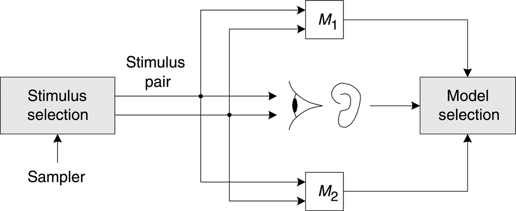
A conventional methodology for selecting the best of two models involves direct comparison of model responses with human two-alternative-forced-choice (2AFC) responses on a set of stimuli, as illustrated in Figure 1. Specifically, for each pair of stimuli, the subject is asked which stimulus is perceived to have a larger value of perceptual quantity q. Average subjective responses are then compared with model responses, and the model (say) that predicts a higher percentage of responses correctly is declared the winner.
Figure 1.
Direct method for model selection.
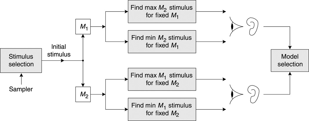
As an alternative, our proposed MAD competition methodology is illustrated in Figure 2. Starting from each of a set of base stimuli, we synthesize stimuli that have maximal/minimal values of one model, while holding the value of the other model constant. This is a constrained optimization problem, and depending on the details of the two models, the solution might be obtained in closed form, or through numerical optimization (e.g., for models that are continuous in the stimulus space, a gradient ascent/descent method may be employed, which is described later). The resulting stimuli may then be compared by human subjects. If the stimuli are easily differentiated in terms of quantity q, then they constitute strong evidence against the model that was held constant. The same test may be performed for stimuli generated with the roles of the two models reversed, so as to generate counterexamples for the other model.
Figure 2.
MAD competition method for model selection.
A toy example
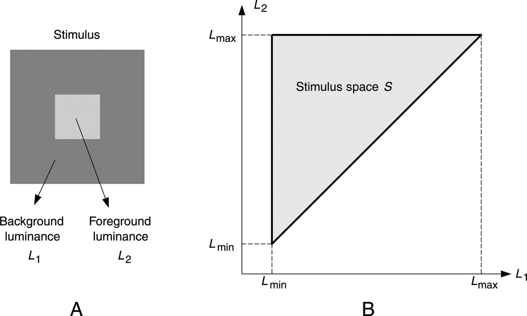
As a simple illustration of the difference between the direct and the MAD competition-based 2AFC methods, we compare two models for the perceived contrast of a test square on a constant-luminance background. An example stimulus is shown in Figure 3A. A square-shaped foreground with uniform luminance L2 is placed at the center of a background of uniform luminance L1. The perceptual quantity q(L1, L2) is the perceived contrast between the foreground and the background. These stimuli live in a two-dimensional parameter space, specified by the pair [L1, L2]. This allows us to depict the problem and solution graphically. Suppose that the maximal and minimal luminance values allowed in the experiment are Lmax and Lmin, respectively. Also assume that the foreground luminance is always higher than the background, i.e., L2 > L1. Then the entire stimulus space can be depicted as a triangular region in a two-dimensional coordinate system defined by L1 and L2, as shown in Figure 3B.
Figure 3.
Illustration of the stimulus and the stimulus space of the contrast perception experiment.
We use MAD to compare two simple models for the perceived contrast q. The first model states that the perceived contrast is determined by the difference between the foreground and the background luminances, i.e., M1 = L2 − L1. In the second model, the perceived contrast is determined by the ratio between the luminance difference and the background luminance, i.e., M2 = (L2 − L1)/L1.
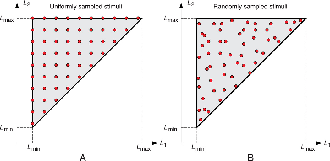
To apply the direct 2AFC method, a large number of stimulus pairs in the stimulus space need to be selected. These specific stimuli may be chosen deterministically, for example, using evenly spaced samples in either linear or logarithmic scale in the stimulus space, as exemplified in Figure 4A. They may also be chosen randomly to adequately cover the stimulus space, as shown in Figure 4B. In either case, it is typical to show them in random order to the subjects. For each pair of stimuli, subjects are asked to report which stimulus has a higher contrast. The results are then compared with the model predictions to see which model can best account for the subjective data.
Figure 4.
Stimulus selection in direct testing methods.
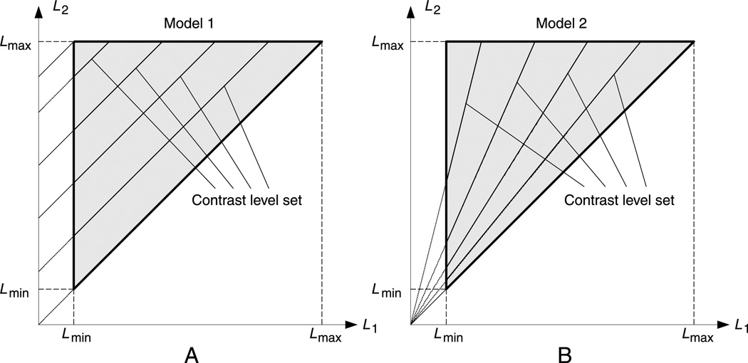
The MAD competition method is explained in Figures 5 and 6. Before applying the MAD competition procedures, it is helpful to visualize the level sets (or equal-value contours) of the models being evaluated in the stimulus space. Specifically, in this contrast perception example, the level sets of models M1 and M2 are always straight lines, which are plotted in Figures 5A and 5B, respectively. The fact that the level sets of the two models are generally not parallel implies that subsets of images producing the same value in one model (i.e., lying along a contour line of that model) will produce different values in the other model.
Figure 5.
Contrast perception models described in the stimulus space.
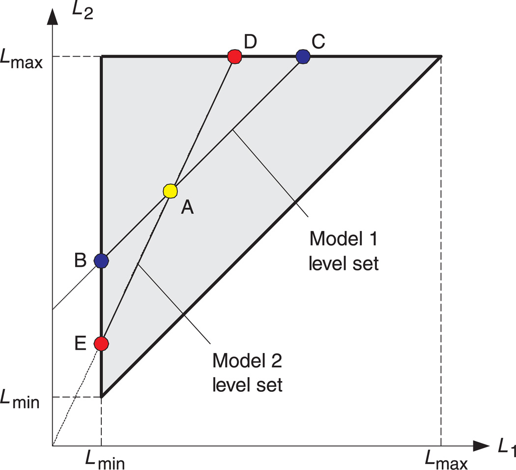
Figure 6.
Stimulus selection in MAD competition method.
Figure 6 illustrates the stimulus synthesis procedure in the MAD competition method. It starts by randomly selecting an initial point in the stimulus space, e.g., . A pair of stimuli with matching M1 but extremal values of M2 is given by
| (1) |
and
| (2) |
and the second pair of stimuli with matching M2 but extremal M1 values is
| (3) |
and
| (4) |
The stimulus pairs (B, C) and (D, E) are subject to visual inspection using a 2AFC method, i.e., the subjects are asked to pick one stimulus from each pair that appears to have higher contrast. This procedure is repeated with different initial points A.
Finally, an overall decision about the winner is made based on an analysis of all 2AFC tests. For example, if M2 is a better model than M1, then the perceived contrast between the (D, E) pairs should be harder to distinguish than the (B, C) pairs. In other words, in the 2AFC test, the percentage of choosing either D or E should be closer to 50%, whereas the percentage of choosing either B or C should be closer to 0% or 100%. In some cases, there may not be a clear winner. For example, if the perceived contrasts between B and C and between D and E are both highly distinguishable, then neither model would provide a good prediction of the visual perception of contrast. In other words, the stimuli generated to extremize one model serve to falsify the other (although their relative degrees of failure may still be different and measurable with MAD competition).
Application to image quality assessment models
The previous example demonstrates the differences between MAD competition and a more conventional model selection approach. However, this example does not provide a compelling justification for the use of MAD, since the stimulus space is only two-dimensional, and thus could have been explored effectively by uniform or random sampling. For models that operate on high-dimensional stimuli (e.g., the pixels of digitized photographic images), a direct examination of samples that cover the space becomes impossible, and the advantage of MAD competition is significant. In this section, we demonstrate this in the context of perceptual image quality.
Image quality models
Image quality models aim to predict human perception of image quality (Pappas, Safranek, & Chen, 2005; Wang & Bovik, 2006). They may be classified into full-reference (where an original “perfect-quality” image is available as a reference), reduced-reference (where only partial information about the original image is available), and no-reference methods (where no information about the original image is available). For our purposes here, we use MAD competition to compare two full-reference image quality models. The first is the mean squared error (MSE), which is the standard metric used throughout the image processing literature. The second is the recently proposed structural similarity index (SSIM; Wang et al., 2004). Definitions of both models are provided in Appendix A. The gradients of MSE and SSIM with respect to the image can be computed explicitly (see Appendix B).
In previous studies, both the MSE and the SSIM models have been tested using “standard” model evaluation techniques. The testing results have been reported for the LIVE image database (http://live.ece.utexas.edu/research/quality), a publicly available subject-rated image quality database with a relatively large number of images corrupted with diverse types of distortions. The database contains 29 high-resolution original natural images and 779 distorted versions of these images. The distortion types include JPEG compression, JPEG2000 compression, white Gaussian noise contamination, Gaussian blur, and transmission errors in JPEG2000 compressed bitstreams using a fast-fading Rayleigh channel model. Subjects were asked to provide their perception of quality on a continuous linear scale and each image was rated by 20–25 subjects. The raw scores for each subject were converted into Z-scores. The mean opinion score and the standard deviation between subjective scores were computed for each image. The video quality experts group (www.vqeg.org) has suggested several evaluation criteria to assess the performance of objective image quality models. These criteria include linear correlation coefficient after non-linear regression, linear correlation coefficient after variance-weighted non-linear regression, rank-order correlation coefficient, and outlier ratio. Details about the evaluation procedure can be found in VQEG (2000). It has been reported in Wang et al. (2004) that the SSIM index significantly outperforms the MSE for the LIVE database, based on these criteria. However, as mentioned earlier, it may not be appropriate to draw strong conclusions from these tests, because the space of images is so vast that even a database containing thousands or millions of images will not be sufficient to adequately cover it. Specifically, the LIVE database is limited in both the number of full-quality reference images and in the number and level of distortion types.
MAD competition
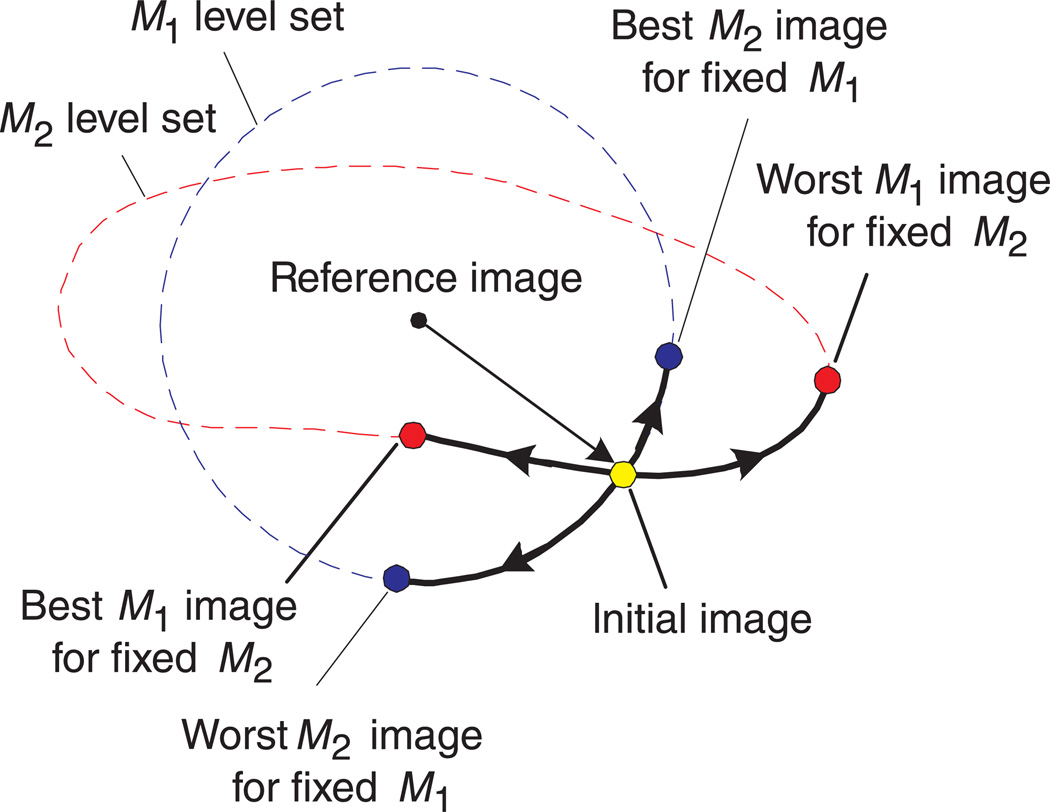
Unlike the contrast perception example of the previous section, the SSIM model is too complex for us to solve for the MAD stimulus pairs analytically. But it is differentiable, and thus allows an alternative approach based on iterative numerical optimization, as illustrated in Figure 7. First, an initial distorted image is generated by adding a random vector in the image space to the reference image. Now consider a level set of M1 (i.e., set of all images having the same value of M1) as well as a level set of M2, each containing the initial image. Starting from the initial image, we iteratively move along the M1 level set in the direction in which M2 is maximally increasing/decreasing. The iteration continues until a maximum/minimum M2 image is reached. Figure 7 also demonstrates the reverse procedure for finding the maximum/minimum M1 images along the M2 level set. The maximally increasing/decreasing directions may be computed from the gradients of the two image quality metrics, as described in Appendix C. This gradient descent/ascent procedure does not guarantee that we will reach the global minimum/maximum on the level set (i.e., we may get “stuck” in a local minimum). As such, a negative result (i.e., the two images are indiscriminable) may not be meaningful. Nevertheless, a positive result may be interpreted unambiguously.
Figure 7.
MAD stimulus synthesis in the image space.
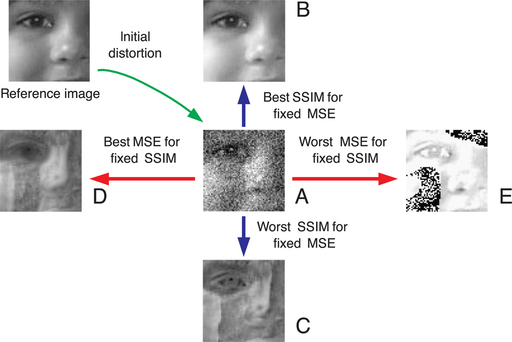
Figure 8 shows an example of this image synthesis process, where the intensity range of the reference image is [0, 255] and the initial image A was created by adding independent white Gaussian noise with MSE = 1024. Visual inspection of the images indicates that both models fail to capture some aspects of perceptual image quality. In particular, images B and C have the same MSE with respect to the reference original image (top left). But image B has very high quality, while image C poorly represents many important structures in the original image. Thus, MSE is clearly failing to provide a consistent metric for image quality. On the other hand, image D and image E have the same SSIM values. Although both images have very noticeable artifacts, the distortions in image E are concentrated in local regions but extremely noticeable, leading to subjectively lower overall quality than image D. Computer animations of MAD competition between MSE and SSIM can be found at http://www.ece.uwaterloo.ca/~z70wang/research/mad/.
Figure 8.
Synthesized images for MAD competition between MSE and SSIM.
2AFC experiments
Although the images in Figure 8 indicate that both of the competing models fail, they fail in different ways, and to different extents. It is also clear that the degree of failure depends on the initial distortion level. When the initial noise level is very small, all four synthesized images are visually indistinguishable from the original image. As the initial noise level increases, failures should become increasingly noticeable. These observations motivate us to measure how rapidly the perceived distortion increases as a function of the initial distortion level.
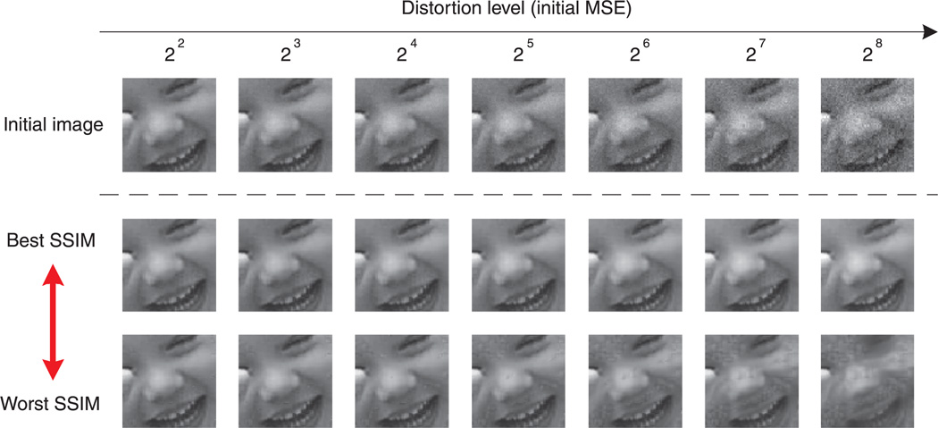
For each reference image, we create the initial distorted images by adding white Gaussian noise, where the noise variance determines the initial distortion level. Specifically, we let for l = 0, 1, 2, …, 9, respectively. For each noise level, we generate four test images (minimum/maximum MSE with the same SSIM and minimum/maximum SSIM with the same MSE) using the iterative constrained gradient ascent/descent procedure described in Appendix C. Sample synthesized images are shown in Figure 9.
Figure 9.
Synthesized images for 2AFC MAD competition experiment.
We used these synthetic images as stimuli in a 2AFC experiment. Subjects were shown pairs of images along with the original image and were asked to pick the one from each pair that had higher perceptual quality. Subjects were allowed to free view the images without fixation control, and no time limit was imposed on the decision. There are all together 10 reference images, each distorted at 10 initial distortion levels, resulting in 200 pairs of synthesized images. These image pairs are shown to the subjects in random order and each pair was shown twice to each subject. Five subjects were involved in the experiments. One was an author, but the others subjects were not aware of the purpose of this study.
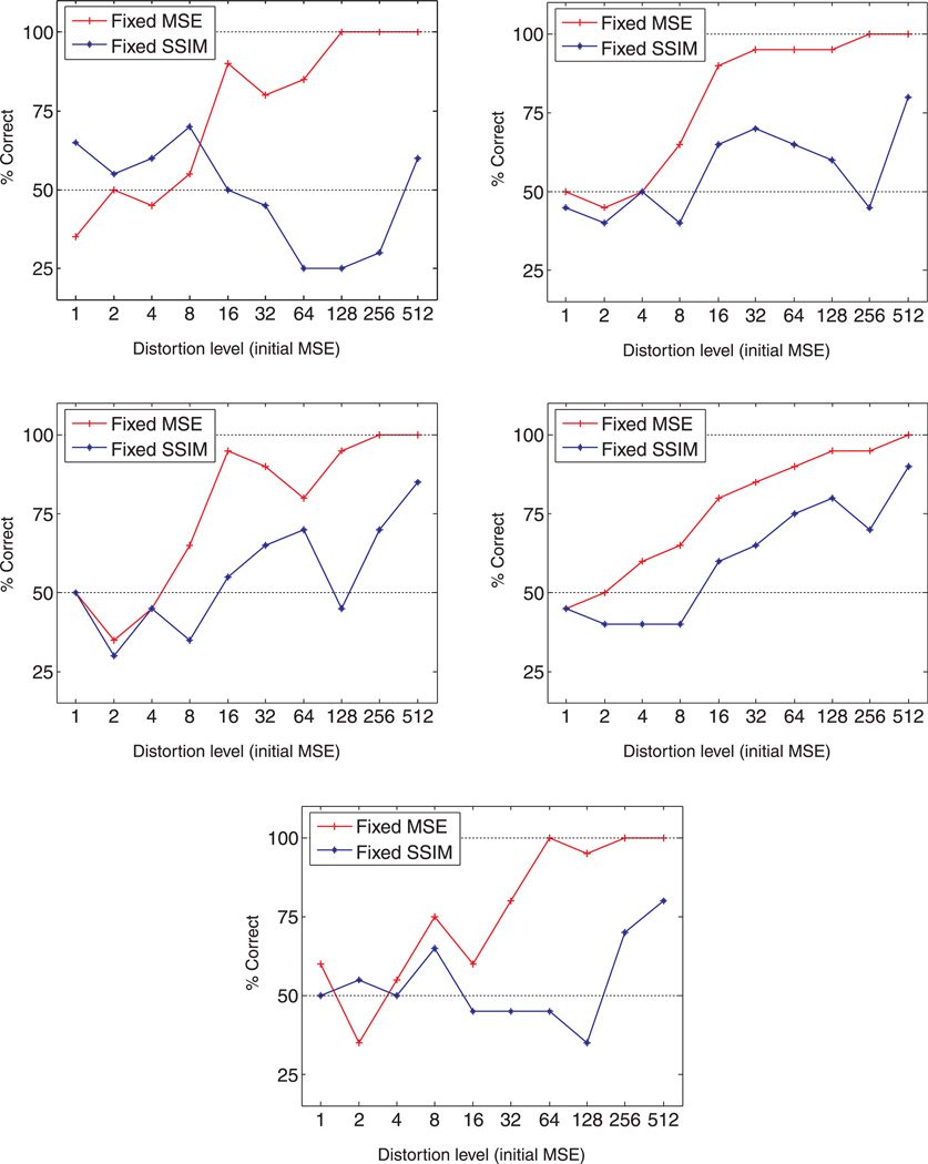
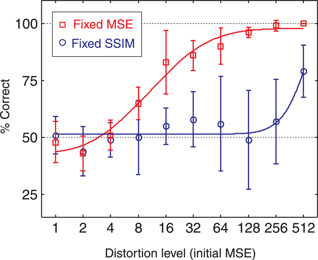
The experimental results for each of the five subjects are shown in Figure 10. Responses are seen to be in general agreement at low distortion levels and for the fixed MSE images at high distortion levels. However, the subjects responded quite differently to the fixed SSIM images at high distortion levels. This is reflected in the average discrimination levels and the error bars of the combined subject data, shown in Figure 11, which is fitted with a Weibull function. At low levels of distortion, all subjects show chance performance for both the SSIM and MSE images. But the fixed MSE images are seen to be much more discriminable than the fixed SSIM images at mid to high levels of distortion. Based on these observations, one may conclude that the SSIM is a better model than the MSE in this MAD competition test, especially when the image distortion level is high.
Figure 10.
2AFC results for each of the five subjects (ZW, CR, AS, TS, DH) involved in the experiments.
Figure 11.
2AFC results for all subjects fitted with Weibull functions.
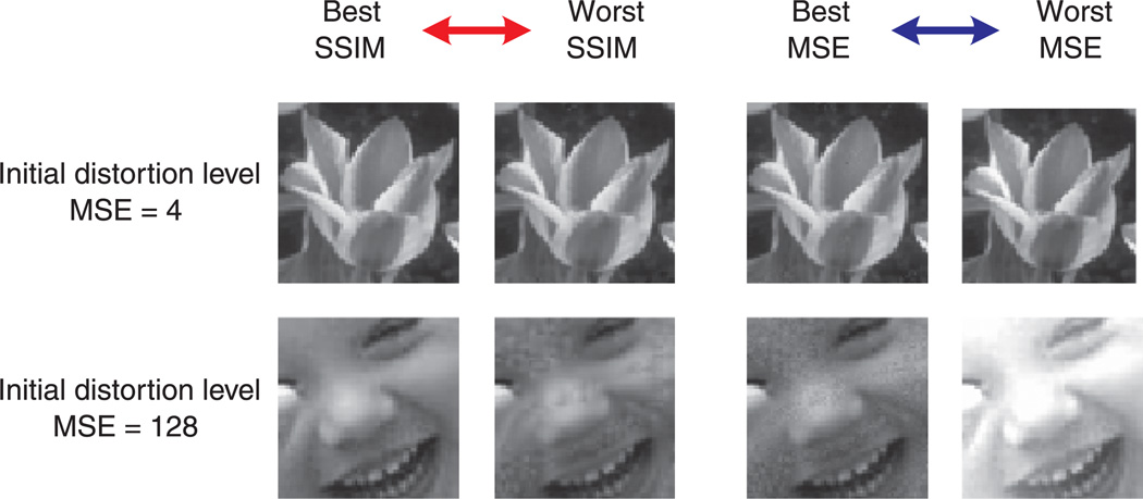
Another interesting observation in Figure 11 is that the fixed SSIM images exhibit substantially more response variability (large error bars) across subjects at high distortion levels. To have a better understanding of this phenomenon, Figure 12 shows four pairs of sample images used in the experiment, two from low initial distortion levels (MSE = 4) and the other two from high initial distortion levels (MSE = 128). At low initial distortion levels, the best/worst SSIM and the best/worst MSE images are visually indistinguishable, resulting in 50% discriminability in 2AFC experiment, as indicated in Figure 11. At high initial distortion level, the best SSIM image has clearly better quality than the worst SSIM image, consistent with reports of all subjects (Figure 11). On the other hand, subjects have very different opinions about the relative quality of the best and worst MSE images, as reflected in the large error bars.
Figure 12.
Sample images at (top) low and (bottom) high initial distortion levels. At initial distortion level (MSE = 4), the best/worst SSIM and the best/worst MSE images are visually indistinguishable, resulting in 50% (chance) discriminability, as shown in Figure 11. At high initial distortion level (MSE = 128), the best SSIM image has clearly better quality than the worst SSIM image (with the same MSE), thus high percentage value was obtained in the 2AFC experiment (Figure 11). On the other hand, subjects have very different opinions about the relative quality of the best and worst MSE images (with the same SSIM), as reflected by the large error bars in Figure 11.
Discussion
We have described a systematic approach, the MAD competition method, for the comparison of computational models for perceptually discriminable quantities. Much of the scientific endeavor is based on experiments that are carefully designed to distinguish between or falsify hypotheses or models. MAD competition provides a means of accelerating this process for a particular type of models, through the use of computer-optimized stimuli. This is particularly useful in cases where the stimulus space is large, and/or the models are complex, so that designing such stimuli by hand becomes nearly impossible. Many methodologies have been developed for automating the selection of stimuli from a low-dimensional parametric family based on the history of responses in an experiment (e.g., Kontsevich & Tyler, 1999; Watson & Pelli, 1983). More recently, methods have been developed for online modification of stimulus ensembles based on previous responses (Machens, Gollisch, Kolesnikova, & Herz, 2005; Paninski, 2005). Our method differs in that it is not response-dependent, and it is not limited to a low-dimensional space, but it does rely on explicit specification of two computational models that are to be compared. MAD also provides an intuitive and effective method to discover the relative weaknesses of competing models and can potentially suggest a means of combining the advantages of multiple models.
It is important to mention some of the limitations of the MAD competition method. First, as with all experimental tests of scientific theories, MAD competition cannot prove a model to be correct: it only offers an efficient means of selecting stimuli that are likely to falsify it. As such, it should be viewed as complementary to, rather than a replacement for, the conventional direct method for model evaluation, which typically aims to explore a much larger portion of the stimulus space. Second, depending on the specific discriminable quantity and the competing models, the computational complexity of generating the stimuli can be quite significant, possibly prohibitive. The constrained gradient ascent/descent algorithms described in Appendix C assume that both competing models are differentiable and that their gradients may be efficiently computed (these assumptions hold for the models used in our current experiments). Third, if the search space of the best MAD stimulus is not concave/convex, then the constraint gradient ascent/descent procedure may converge to local maxima/minima. More advanced search strategies may be used to partially overcome this problem, but they typically are more computationally costly, and still do not offer guarantees of global optimality. Nevertheless, the locally optimal MAD stimuli may be sufficient to distinguish the two competing models. Specifically, if the generated stimuli are discriminable, then they will still serve to falsify the model that scores them as equivalent. Fourth, MAD-generated stimuli may be highly unnatural, and one might conclude from this that the application scope of one or both models should be restricted. Finally, there might be cases where the extremal stimuli of each model succeed in falsifying the other model. Alternatively, each of the models could be falsified by the other in a different region of the stimulus space. In such cases, we may not be able to reach a conclusion that one model is better than the other. However, such double-failure results in MAD competition are still valuable because they can reveal the weaknesses of both models and may suggest potential improvements.
Although we have demonstrated the MAD competition method for two specific perceptual quantities–contrast and image quality–the general methodology should be applicable to a much wider variety of examples, including higher level cognitive quantities (e.g., object similarity, aesthetics, emotional responses), and to other types of measurement (e.g., single-cell electrode recordings or fMRI).
Appendix A
Definitions of image quality models
Two image quality models, mean square error and the structural similarity index, are used in our experiment.
Mean squared error (MSE)
For two given images X and Y (here an image is represented as a column vector, where each entry is the grayscale value of one pixel), the MSE between them can be written as
| (A1) |
where NI is the number of pixels in the image.
Structural similarity index (SSIM)
The SSIM index (Wang et al., 2004) is usually computed for local image patches, and these values are then combined to produce a quality measure for the whole image. Let x and y be column vector representations of two image patches (e.g., 8 × 8 windows) extracted from the same spatial location from images X and Y, respectively. Let μx, , and σxy represent the sample mean of the components of x, the sample variance of x, and the sample covariance of x and y, respectively:
| (A2) |
where NP is the number of pixels in the local image patch and 1 is a vector with all entries equaling 1. The SSIM index between x and y is defined as
| (A3) |
where C1 and C2 are small constants given by C1 = (K1R)2 and C2 = (K2R)2, respectively. Here, R is the dynamic range of the pixel values (e.g., R = 255 for 8 bits/pixel grayscale images), and K1 ≪ 1 and K2 ≪ 1 are two scalar constants (K1 = 0.01 and K2 = 0.03 in the current implementation of SSIM). It can be easily shown that the SSIM index achieves its maximum value of 1 if and only if the two image patches x and y being compared are exactly the same.
The SSIM index is computed using a sliding window approach. The window moves pixel by pixel across the whole image space. At each step, the SSIM index is calculated within the local window. This will result in an SSIM index map (or a quality map) over the image space. To avoid “blocking artifacts” in the SSIM index map, a smooth windowing approach can be used for local statistics (Wang et al., 2004). However, for simplicity, we use an 8 × 8 square window in this paper. Finally, the SSIM index map is combined using a weighted average to yield an overall SSIM index of the whole image:
| (A4) |
where xi and yi are the ith sampling sliding windows in images X and Y, respectively, W(xi, yi) is the weight given to the ith sampling window, and NS is the total number of sampling windows. NS is generally smaller than the number of image pixels NI to avoid the sampling window exceed the boundaries of the image. The original implementations of the SSIM measure corresponds to the case of uniform pooling, where W(x, y) ≡ 1. In Wang and Shang (2006), it was shown that a local information content-weighted pooling method can lead to consistent improvement for the image quality prediction of the LIVE database, where the weighting function is defined as
| (A5) |
This weighting function was used for the examples shown in this article.
Appendix B
Gradient calculation of image quality models
In order to apply the constrained gradient ascent/descent algorithm (details described in Appendix C), we need to calculate the gradients of the image quality models with respect to the image. Here the gradients are represented as column vectors that have the same dimension as the images.
Gradient of MSE
For MSE, it can be easily shown that
| (B1) |
Gradient of SSIM
For SSIM, taking the derivative of Equation A4 with respect to Y, we have
| (B2) |
where
| (B3) |
and
| (B4) |
Thus, the gradient calculation of an entire image is converted into weighted summations of the local gradient measurements. For a local SSIM measure as in Equation A3, we define
| (B5) |
Then it can be shown that
| (B6) |
where 1 denotes a column vector with all entries equaling 1. For the case that W(x, y) ≡ 1, we havel ∇⃑YW(x, y) ≡ 0 in Equations B3 and B4. Therefore,
| (B7) |
In the case of local information content-weighted average as in Equation A5, we have
| (B8) |
Thus, ∇⃑YS(X, Y) can be calculated by combining Equations A3, B2, B3, B4, B6, and B8.
Appendix C
Constrained gradient ascent/descent for image synthesis
Here we describe the iterative constrained gradient ascent/descent algorithm we implemented to synthesize images for MAD competition.
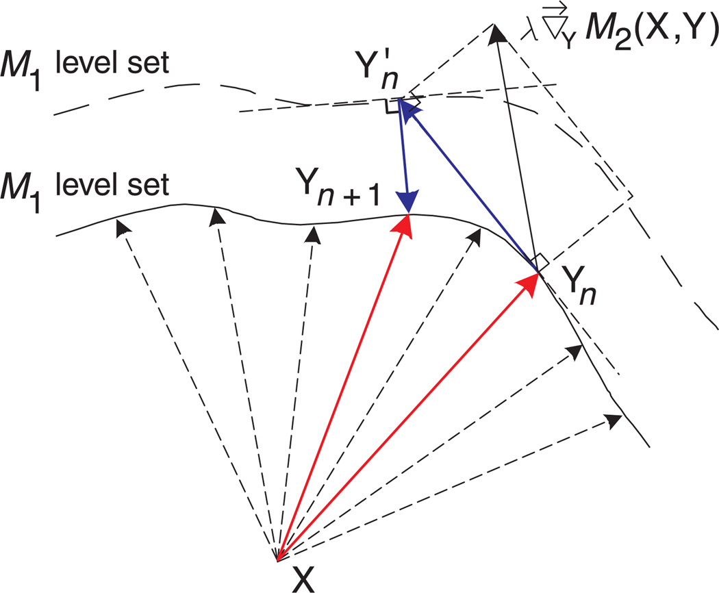
Figure C1 illustrates a single step during the iterations, where the goal is to optimize (find maxima and minima) M2 while constrained on the M1 level set. We represent images as column vectors, in which each entry represents the grayscale value of one pixel. Denote the reference image X and the synthesized image at the nth iteration Yn (with Y0 representing the initial image). We compute the gradient of the two image quality models (see Appendix B), evaluated at Yn:
| (C1) |
and
| (C2) |
We define a modified gradient direction, Gn, by projecting out the component of G2,n, that lies in the direction of G1,n:
| (C3) |
A new image is computed by moving in the direction of this vector:
| (C4) |
Finally, the gradient of M1 is evaluated at , and an appropriate amount of this vector is added in order to guarantee that the new image has the correct value of M1:
| (C5) |
such that
| (C6) |
For the case of MSE, the selection of ν is straightforward, but in general it might require a one-dimensional (line) search.
Figure C1.
Illustration of the nth iteration of the gradient ascent/descent search procedure for optimizing M2 while constraining on the M1 level set.
During the iterations, the parameter λ is used to control the speed of convergence and ν must be adjusted dynamically so that the resulting vector does not deviate from the level set of M1. The iteration continues until the image satisfies certain convergence condition, e.g., mean squared change in the synthesized image in two consecutive iterations is less than some threshold. If metric M2 is differentiable, then this procedure will converge to a local maximum/minimum of M2. In general, however, we have no guaranteed means of finding the global maximum/minimum (note that the dimension of the search space is equal to the number of pixels in the image), unless the image quality model satisfies certain properties (e.g., convexity or concavity). In practice, there may be some additional constraints that need to be imposed during the iterations. For example, for 8 bits/pixel grayscale images, we may need to limit the pixel values to lie between 0 and 255.
Footnotes
Commercial relationships: none.
Contributor Information
Zhou Wang, Department of Electrical and Computer Engineering, University of Waterloo, Waterloo, ON, Canada.
Eero P. Simoncelli, Howard Hughes Medical Institute, Center for Neural Science, and Courant Institute of Mathematical Sciences, New York University, New York, NY, USA
References
- Faugeras OD, Pratt WK. Decorrelation methods of texture feature extraction. IEEE Transactions on Pattern Analysis Machine Intelligence. 1980;2:323–332. doi: 10.1109/tpami.1980.4767031. [DOI] [PubMed] [Google Scholar]
- Gagalowicz A. A new method for texture fields synthesis: Some applications to the study of human vision. IEEE Transactions on Pattern Analysis Machine Intelligence. 1981;3:520–533. doi: 10.1109/tpami.1981.4767145. [DOI] [PubMed] [Google Scholar]
- Heeger D, Bergen J. Pyramid-based texture analysis/synthesis. Proceedings of the ACM SIGGRAPH. 1995:229–238. [Google Scholar]
- Kontsevich LL, Tyler CW. Bayesian adaptive estimation of psychometric slope and threshold. Vision Research. 1999;39:2729–2737. doi: 10.1016/s0042-6989(98)00285-5. [PubMed] [DOI] [PubMed] [Google Scholar]
- Machens CK, Gollisch T, Kolesnikova O, Herz AV. Testing the efficiency of sensory coding with optimal stimulus ensembles. Neuron. 2005;47:447–456. doi: 10.1016/j.neuron.2005.06.015. [PubMed] [Article] [DOI] [PubMed] [Google Scholar]
- Paninski L. Asymptotic theory of information–Theoretic experimental design. Neural Computation. 2005;17:1480–1507. doi: 10.1162/0899766053723032. [PubMed] [DOI] [PubMed] [Google Scholar]
- Pappas TN, Safranek RJ, Chen J. Perceptual criteria for image quality evaluation. In: Bovik A, editor. Handbook of image and video processing. Elservier Academic Press; 2005. pp. 939–960. [Google Scholar]
- Portilla J, Simoncelli EP. A parametric texture model based on joint statistics of complex wavelet coefficients. International Journal of Computer Vision. 2000;40:49–71. [Google Scholar]
- Teo PC, Heeger DJ. Perceptual image distortion. Proceedings of SPIE. 1994;2179:127–141. [Google Scholar]
- VQEG. Final report from the video quality experts group on the validation of objective models of video quality assessment. 2000 http://www.vqeg.org. [Google Scholar]
- Wang Z, Bovik AC. A universal image quality index. IEEE Signal Processing Letters. 2002;9:81–84. [Google Scholar]
- Wang Z, Bovik AC. Modern image quality assessment. Morgan & Claypool; 2006. [Google Scholar]
- Wang Z, Bovik AC, Sheikh HR, Simoncelli EP. Image quality assessment: From error visibility to structural similarity. IEEE Transactions on Image Processing. 2004;13:600–612. doi: 10.1109/tip.2003.819861. [PubMed] [DOI] [PubMed] [Google Scholar]
- Wang Z, Shang X. Spatial pooling strategies for perceptual image quality assessment; Proceedings of the IEEE International Conference on Image Processing; 2006. pp. 2945–2948. [Google Scholar]
- Wang Z, Simoncelli EP, Bovik AC. Multi-scale structural similarity for image quality assessment. Proceedings of the IEEE Asilomar Conference on Signals, Systems & Computers. 2003;2:1398–1402. [Google Scholar]
- Watson AB, Pelli DG. QUEST: A Bayesian adaptive psychometric method. Perception & Psychophysics. 1983;33:113–120. doi: 10.3758/bf03202828. [PubMed] [DOI] [PubMed] [Google Scholar]
- Zhu S-C, Wu YN, Mumford D. FRAME: Filters, random fields and maximum entropy–Towards a unified theory for texture modeling. International Journal of Computer Vision. 1998;27:1–2. [Google Scholar]


