Polyoma virus capsid structure at 22.5 Å resolution

Abstract

X-ray diffraction data from polyoma capsid crystals were phased by refinement of low-resolution starting models to obtain a self-consistent structural solution. The unexpected result that the hexavalent morphological unit is a pentamer shows that specificity of bonding is not conserved among the protein subunits in the icosahedrally symmetric capsid.

X-RAY crystallographic studies on polyoma virus were begun to visualize the protein subunit packing in the icosahedral capsid and to explore the way in which the chromatin core of this tumorigenic virus is packaged inside its protein shell¹. Analysis of electron micrographs has established that the capsid consists of 12 five-coordinated and 60 six-coordinated morphological units² (capsomeres) arranged on a T = 7d icosahedral surface lattice³ (Fig. 1). It has been presumed, based on the principles formulated to account for the morphology and chemical composition of simple icosahedral virus particles⁴, that the capsids of the T = 7 papova viruses should be constructed from 420 identical protein subunits quasi-equivalently bonded into 12 pentameric and 60 hexameric capsomeres. High-resolution X-ray structure determination of tomato bushy stunt virus⁵ and southern bean mosaic virus⁶ has established that quasi-equivalence is used to conserve essential bonding specificity among the 180 chemically identical subunits of these T = 3 icosahedral capsids. Our 22.5-Å resolution electron density map of the polyoma capsid reveals unexpected substructure in the hexavalent capsomere that is inconsistent with the expectation of quasi-equivalent bonding of identical subunits. (The adjectives ‘hexavalent’ and ‘pentavalent’ are introduced to identify the six- and five-coordinated morphological units without prejudging the nature of their substructure.)

Fig. 1.

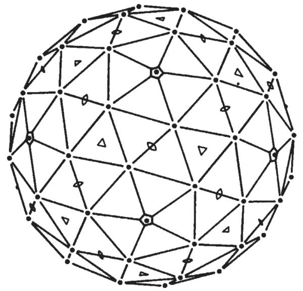
T = 7d icosahedral surface lattice with five-, three- and two-fold axes marked. The drawing shows one side of the polyhedral surface consisting of 60 six-coordinated and 12 five-coordinated lattice points at the same radius. The location of the six-coordinated point is that determined for the hexavalent morphological unit in the polyoma capsid.

The starting point for our analysis of the polyoma capsid diffraction data was a model representing the coarse surface features seen in the three-dimensional image reconstruction from electron micrographs of negatively stained particles³. The capsomeres in this image reconstruction appear as hollow, stubby protrusions with no regular substructure, about 50 Å in diameter and separated from their nearest neighbours by 80–90 Å at a radius of 200 Å in the capsid. Pentavalent and hexavalent morphological units appear to be about the same size, which would not be expected if they were composed of pentamers and hexamers of identical protein subunits.

Cells infected with polyoma virus and other papova viruses produce, in addition to intact virions and empty capsids, hollow tubular particles that appear to be polymorphic assemblies of the capsomeres⁷. There are two categories of tube: wide tubes, about the diameter of the virion, which are built of capsomeres arranged in a hexagonal surface lattice, and narrow tubes, which Kislev and Klug⁸ showed to be constructed of pentameric capsomeres arranged in a lattice they called a ‘pentagonal tessellation’. The capsomeres of the wide tubes were presumed to be hexamers but the chemical and structural relationships between the morphological units of the ‘hexamer’ and ‘pentamer’ tubes could not be established at that time. In the light of our results new questions are raised about the structure of these polymorphic assemblies of the capsid subunits.

Complete virions contain seven different proteins, four of which are cellular histones associated with the DNA, the other three (VP1, VP2 and VP3) being virus coded⁹. VP1 (molecular weight (MW) ~42,000) is the major capsid protein. The function of VP2 and VP3 (MW ~35,000 and ~23,000, respectively), which constitute less than 20% of the virion proteins, is not clear. Purified capsids have been prepared that contain only VP1¹⁰ and these particles have normal morphology. Thus, the pentavalent and hexavalent capsomeres seem to be built of identical VP1 subunits.

Crystallography

Polyoma virus capsids of the strain Sp-34 were isolated as previously described¹¹. The preparation used for growing crystals consisted predominantly of the major capsid protein, VP1, and only a small amount of VP2 and VP3 compared with the intact virion. Crystals, in the rhombic dodecahedral form¹², were grown by equilibrating a solution of polyoma virus capsids at 4 mg ml⁻¹ in 0.02 M Tris pH 9.5 and 0.17 M sodium sulphate against 0.55 M sodium sulphate by vapour diffusion. Crystals grew over a period of 1 month at room temperature. These crystals diffracted to a resolution of at least 8 Å. The icosahedral capsids, of packing diameter 495 Å, are located at the centre and corners of the b.c.c. lattice (space group I23, unit cell edge 572 Å) with particle two- and three-fold axes coincident with the crystallographic axes¹. Diffraction data were collected to 22.5 Å resolution by screened precession photography (crystal-to-film distance 150 mm) with an Elliott GX6 rotating anode X-ray generator using a 0.2-mm focal cup and two perpendicular-focusing mirrors¹³. A total of 11 zero level (μ = 2°) and 4 upper level (μ = 1.5°) photographs were collected, each a 48-h exposure. These gave 1,481 independent reflections between (1/150) and (1/22.5) Å spacing, representing 94% of the data within this resolution range. The individual films were digitized on an Optronics P1000 densitometer at 50 μm scanning raster and processed using a modified version of the Harvard Scan-11 system on a PDP-11/40 computer. The films scaled together with an R factor measuring the mean variation in intensity of symmetry-related reflections of 5.7%.

Models for phase refinement

Trial phases, calculated to 30 Å resolution from models based on information from electron microscopy³ and small-angle X-ray diffraction¹, were refined and extended to 22.5 Å resolution by imposing the constraints of non-crystallographic symmetry and solvent flattening. This approach is similar to that used to determine the structure of southern bean mosaic virus to 22.5 Å resolution¹⁴. Our starting model of the polyoma capsid, consisting of 72 morphological units arranged in a T = 7d icosahedral surface lattice (Fig. 1), is a non-centrosymmetric structure. Consequently, calculated trial phases will introduce the non-centric component of the structure factors from the start. This is essential to the quality of the subsequent real-space phase refinement and extension.

Models consisting of 72 hollow cylindrical capsomeres on a spherical shell were formulated with 9 adjustable parameters defining the size and position of the structural elements. Phases from these models were calculated by Fourier transforming a density map generated in a lattice corresponding to the polyoma crystal. The model parameters were adjusted by comparing the calculated and observed structure factor amplitudes. The models which gave the best R factor fit were built from morphological units about 40 Å high and 80 Å in diameter with a 35-Å diameter axial hole, resting on a shell extending from a radius of 180–200 Å. The effect of moving the hexavalent morphological unit in this model is shown in Fig. 2, where the R factor is plotted as a function of position. The position of the minimum is close to the hexavalent capsomere location observed in Finch’s image reconstruction from electron micrographs³. A projection of this ‘best’ model down a two-fold axis is shown in Fig. 3a. The R factor for this model to 30 Å resolution was 50% where R is defined as

$$\mathit{R}=\frac{\Sigma \Vert {\mathit{F}}_0\mid -\mid {\mathit{F}}_c\Vert }{\Sigma \mid {\mathit{F}}_0\mid }\times 100$$

where ȣF_oȣ and ∣F_c∣ are observed and calculated structure factor amplitudes. The R factor as a function of resolution is shown in Fig. 4a.

Fig. 2.

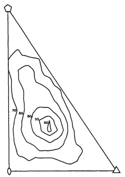
Location of the hexavalent unit in the icosahedral surface lattice. The R factor comparing the calculated and measured diffraction pattern is plotted as a function of the position of the hexavalent unit in the icosahedral cell defined by the five-, three-and two-fold axes (see Fig. 1). The model giving the smallest R factor is shown in Fig. 3a.

Fig. 3.

Density maps of the top half of particles (diameter 495 Å) projected down a two-fold axis (orientation as in Fig. 1). The maps were scaled to have the same total electron density and were photographed directly from a 256 grey scale TV graphics display. a, Model map at 30 Å resolution; b, map computed using observed data and model phases to 30 Å resolution without refinement; c, 30 Å resolution refined map; d, refined map at 22.5 Å resolution calculated by phase extension from 30 Å. Note how the substructure in the morphological units develops as the refinement proceeds. Even at 30 Å resolution the hexavalent unit has a pentagonal appearance.

Fig. 4.

R factors comparing the agreement between observed and calculated structure factor amplitudes, a, As a function of resolution comparing initial model and refined map at 30 Å resolution; b, as a function of refinement cycle at 30 Å resolution; c, as a function of resolution for the phase extension from 30 to 22.5 Å resolution; d, as a function of intensity for the 22.5 Å refined map. For a and c the points are plotted so that the interval between points corresponds to equal volume increments in reciprocal space. The starting model (Fig. 3a) fits the observed data best in the 40–50 Å resolution range where there is a strong modulation in the transform determined by the surface lattice arrangement of the morphological units¹. After 14 cycles of refinement (b) there is a substantial improvement in the fit between the calculated and observed amplitudes at low resolution (a). The structure amplitudes phased by extension from 30 to 22.5 Å resolution represent over half of the total data to this resolution. The R factors for these higher resolution data (c) are uniformly satisfactory. The phase extension also leads to an improvement in the R factor for the data to 30 Å resolution by reducing series termination effects. Plotting the R factor of the 1,343 non-zero reflections as a function of intensity (d) shows that there is a correlation between the R factors and the accuracy of the data which are more precise for the stronger reflections.

Particle envelope

Flattening the solvent regions of the electron density map places a powerful constraint on the low resolution phases and also provides the basis for phase extension. Thus, the envelope chosen to enclose the virus capsid is critical in the phase refinement and extension. The envelope used was a spherical shell extending from 165 Å to 260 Å truncated by planes perpendicular to the icosahedral three-fold axes 247 Å from the virus centre. These boundary planes bisect the line of contact between virus particles along the crystallographic three-fold axes. The three hexavalent units adjacent to the crystallographic three-fold axis make contact tip to tip with the related set on the neighbouring particle. As there is no discernible interdigitation of the capsomeres at this resolution, the boundary planes perpendicular to the three-fold axes define the volume associated with one virus particle.

Solvent density for both the interior and exterior of the capsid was taken as the average observed density of the shell extending from 160 to 165 Å. This approach was used because omitting unmeasured low-resolution <(1/150) Å reflections in the initial calculations results in spurious electron density ripples inside the capsid. When the average density of the total solvent region defined by the particle envelope was used as suggested by Bricogne¹⁵, the refinement calculation converged more slowly. Nevertheless, both methods of determining the solvent density gave very similar final values.

Refinement method

The calculated phases from the model structures were refined to 30 Å resolution against the observed structure factor amplitudes by imposing the constraints of solvent flattening and the five-fold non-crystallographic symmetry^15–17. An electron density map was calculated to 30 Å resolution using the model phases and observed amplitudes, and averaged over the five non-crystallographic asymmetric units within the particle envelope. The observed amplitudes were weighted according to their fit to those calculated from the model according to the scheme

$$\mathit{W}=\exp \left(-\frac{\mid {\mathit{F}}_0\mid -\mid {\mathit{F}}_c\mid }{\mid {\mathit{F}}_0\mid }\right)$$

This simple weighting scheme gave faster convergence than that suggested by Sim¹⁸, but the final phase set was not sensitive to the weighting procedure used.

The averaged, solvent-flattened density map was Fourier transformed to calculate phases and amplitudes for the first cycle of refinement; the r.m.s. phase difference and R factor comparing initial and refined structure factors were evaluated; refined phases were combined with measured amplitudes to initiate the next cycle of refinement; these calculations were iterated until the calculated phase difference and R factor did not change significantly from one cycle to the next.

There are two possible orientations for the icosahedral five-fold axis in the I23 unit cell. The orientation used was that indicated by the intensity spikes in the diffraction patterns¹. If the alternative orientation of the five-fold axis was chosen, the R factor between refined and observed structure factors never dropped below 50%. The standard deviation in the density between the five icosahedral units in the crystallographic asymmetric unit for the correct orientation was 1/7th of that calculated for the alternative.

Omission of the unmeasured data below (1/150) Å spacing systematically lowers the calculated amplitudes for the observed structure factors below (1/100) Å spacing. The amplitudes of the innermost observed reflections are the largest in the data set and dominate the scaling of the calculated to the observed structure factors. This effect was mitigated by including the calculated values for the unmeasured data after the fourth cycle with a weight of 0.9. Reduced weighting was applied to avoid divergence of these large terms in the iterative refinement. Various test calculations have established that the low order data can be accurately estimated from the higher resolution data. Without the eight calculated values for the missing low order data, the refinement converged to only 27% as compared with 10.5% with these data after 14 cycles of phase refinement.

Figures 3a–c and 4b illustrate the progress of the refinement in real and reciprocal space. Figure 4b shows the R factors as a function of refinement cycle. Figure 3a represents the starting model to 30 Å resolution, Fig. 3b the unrefined structure calculated from the observed amplitudes with model phases, and Fig. 3c the refined structure at 30 Å resolution.

Tests of refinement method

There is no established criterion for determining the correctness of the electron density map described subsequently. Because the map shows unexpected features, considerable effort was devoted to demonstrate the uniqueness of the refinement. Phases from any model consisting of 72 bumps distributed on the surface of a spherical shell, in a manner consistent with the image from electron microscopy³, refined to the same solution. Indeed, a starting model which placed 60 hemispheres close to the location of the hexavalent units on a spherical shell with no density protruding on the five-fold axes (initial R factor = 65%) refined to the same phase set as the more realistic models, although it took 18 cycles of refinement. Furthermore, phases from elaborate models with hexavalent morphological units containing either five- or six-fold substructure refined to the same final structure.

The reliability of the refinement method was tested by using amplitudes calculated from models in place of observed data. Because the model structure factor calculations give both the amplitude and the phase, it is possible to judge absolutely how well another set of trial phases converges to the correct values. In the test calculations, amplitudes from various T = 7 capsid models were combined with phases from models with different morphology; refinement of the phases always converged to the phases of the model from which the amplitudes were taken. For example, refining initial phases from an all-pentamer T = 7 model against the amplitudes from a 60 hexmer + 12 pentamer model led back to the phases of the model built with hexamers. Thus, our refinement procedure recovers the correct structure corresponding to the amplitudes of the data even when trial starting phases were chosen to attempt to bias the calculation to produce an incorrect result.

Phase extension

The polyoma diffraction data between 30 and 22.5 Å resolution were phased by extension from the refined 30 Å phases. This was necessary because the model phases are only reliable to ~30 Å resolution. Attempts to refine the data directly to 22.5 Å resolution using trial model phases did not converge satisfactorily.

Phase extension is possible because imposition of the envelope on the electron density generates phase information for reflections just beyond the resolution of those used to calculate the map. The characteristics of phase extension were tested using model structure factors and phases in place of the real polyoma diffraction data. Starting from 30 Å resolution, using calculated amplitudes and phases as test data, it was possible to extend and refine the phases to 22.5 Å resolution. The r.m.s. phase difference between the correct and the refined extended phases were generally less than 30°.

The resolution of the actual data refinement was extended from 30 Å to 22.5 Å over 18 cycles. Predicted phases for structure factors within one reciprocal lattice distance (1/572) Å of the previous resolution were included in alternate cycles. The final R factor between observed and calculated structure factor amplitudes was 14.2%. Figure 3d shows a projection down a two-fold axis of half a virus particle excised from the refined map at 22.5 Å resolution and an analysis of the R factor as a function of resolution and intensity at 22.5 Å resolution is shown in Fig. 4c, d.

Electron density map

Figure 5, comparing views of half a virus particle down the icosahedral five-fold axis with that down the axis of a hexavalent morphological unit, reveals a striking similarity between the penta- and hexavalent morphological units. Indeed, the hexavalent capsomere shows a distinctive five-fold character, not six-fold as would be expected from a T = 7 icosahedral surface lattice consisting of 60 T quasi-equivalent structure units (Fig. 1).

Fig. 5.

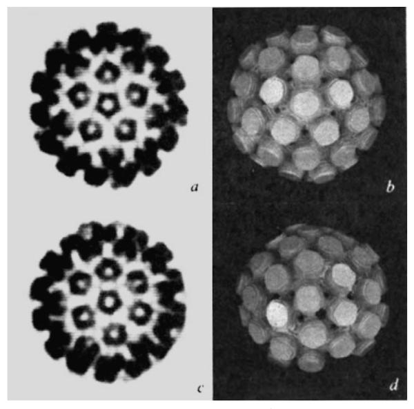
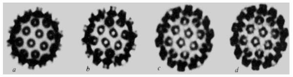
Views of half the capsid (495 Å diameter) down the five-fold axis (a, b) and down the axis of the hexavalent unit (c, d). a And c are computer graphics projections of the electron density map at 22.5 Å resolution, b and c are photographs of a model of stacked sections of the map at 30 Å resolution with the external contour level set at 0.2 of the maximum density. The half-model was built symmetric about the five-fold axis (b), thus, when it is tilted to view down the hexavalent unit (d) the bottom portion of the image is incomplete.

Power spectra of the cylindrical harmonics in sections through the penta- and hexavalent units are shown in Fig. 6. This harmonic analysis demonstrates the structural similarity between the two types of capsomeres as a function of their radial coordinates, in particular, the dominant five-fold substructure of the hexavalent unit. Icosahedral symmetry requires the 12 identical pentavalent units to have five-fold symmetry and the 60 hexavalent units to be identical; but there are no constraints on the size, shape or symmetry of the hexavalent unit. The similarity of the pentavalent and hexavalent capsomeres seen in the electron density map cannot be an artefact of the imposition of the non-crystallographic symmetry in the phase refinement. Thus, our results indicate that all 72 capsomeres are pentameres of identical or very similar subunits.

Fig. 6.

Rotational power spectra of the pentavalent and hexavalent units. a, P_t is the sum of all cylindrical harmonics in sections of the map through the capsomeres normal to the five-fold axis and the ‘best’ axis of the hexavalent units, plotted as a function of the distance of the section from the centre of the particle. b, Relative strength of the five-fold harmonic of the pentavalent unit and the five- and six-fold harmonic of the hexavalent unit. P_t is proportional to the integrated density in each section. At small radii in the capsid a cylindrical boundary of 93 Å diameter was chosen for calculating the power spectrum of the capsomeres. These cylinders touch at a radius of 170 Å. The integrated density of the inner portions of the capsomere may be underestimated by the methods of calculation. The correspondence in the rotational power spectra distribution of the pentavalent and hexavalent units indicates a close similarity in their structures and a small difference in their radial positions. The relative strength of the order 5 harmonic for the outer portion of both the pentavalent and hexavalent capsomere is reduced because the cylindrically symmetric component, which is the dominant term in P_t, is very strong for this part of the structure. The order 5 harmonic for the hexavalent capsomere is always much stronger than that of order 6 (or any other non-zero harmonic).

The electron density map may be divided into two regions: the protruding pentagonal caps and the basal parts connecting capsomeres. The contacts between capsomeres extend inward from ~210 Å radius of the capsid. The protruding caps are ~85 Å in diameter and extend out ~40 Å. The central hole in the capsomere has a diameter of 40 Å at a radius of 210 Å and tapers shut 15 Å from the surface, leaving a dimple on the top of the cap. The basal parts of the capsomeres extend in ~40 Å.

The similarity of the pentavalent and hexavalent morphological units seen in the electron density map, together with the chemical evidence for one kind of protein subunit, indicates that the capsid is built of 360 VP1 molecules. The radial extent of the capsid measured from the electron density map implies a protein subunit ~80 Å long. The dimensions of the wall of the pentagonal cap indicate a subunit diameter in the range 30–40 Å. An ellipsoidal subunit with these dimensions has a volume compatible with that expected for a 42,000-MW protein.

Molecular weight

All the available MW measurements are consistent with a capsid built of 360 VP1 subunits and inconsistent with a 420-subunit structure. The MW of the empty capsid, determined by sedimentation equilibrium¹⁰, is 15 ± 1 × 10⁶, which agrees with the total weight of VP1 in the intact virion estimated from its MW and composition. Furthermore, the MW of 221,000 measured for isolated capsomeres¹⁹ corresponds to a 15.9 × 10⁶-MW capsid built of 72 identical capsomeres, in accord with the direct measurement. The calculated MW of VP1 for a 15 ± 1 × 10⁶-MW capsid consisting of 420 subunits would be 35,700 ± 7%, or 41,700 ± 7% for 360 copies. The calculated MW of VP1 from the DNA sequence is 42,834 (ref. 20) and 42,458 (ref. 21) for two strains of polyoma virus. These sequence values are upper limits because the protein in the capsid may be smaller due to possible post-transcriptional or post-translational processing. Estimates for the MW of VP1 from SDS-gel electrophoresis range from 42,000 to 50,000 but are not very reliable because of dependence on gel concentration¹⁰. Measurement by gel exclusion chromatography of VP1 dissociated with guanidine hydrochloride chloride gives a MW of 41,400 (ref. 10). Although there is no definitive MW measurement for the VP1 subunit in the capsid, all measured values are greater than or close to that expected for 360 subunits, and the smallest measured values are at least 15% larger than expected for 420 subunits.

Protein–subunit interactions

The electron density map provides information about subunit interactions even though the protein subunits themselves are not sharply resolved. Figure 7a and b are sections through the hexavalent and pentavalent capsomeres above the level at which they make contact with each other. It is evident that the projecting portions of the two kinds of capsomeres have very similar pentagonal substructure, indicating that the bonding specificity of the projecting parts of the structure units is conserved. This is analogous to the situation in the tomato bushy stunt virus structure⁵ where bonding specificity is conserved within the two types of protruding dimer domains.

Fig. 7.

Sections of the electron density map showing substructure of the capsomeres (a–d) and drawings on a polyhedral surface (e, f) illustrating an inferred packing relation of structure units. Upper row: views down five-fold axis and lower row: views down axis of hexavalent capsomere. Width of sections displayed 215 Å. Orientation as in Fig. 5. Grey scales at the bottom show the relation between darkness in the images and map density that increases uniformly from left to right of the scales. a, b, Maps of section planes 215 Å above centre of capsid. At this level and above there is little detectable contact between neighbouring capsomeres. c, d, Maps (displayed with enhanced contrast) of section planes 195 Å above centre. At this level and below five basal parts of the capsomeres splay out and contact basal parts of neighbouring capsomeres. Section planes are perpendicular to the axis of the central capsomere and slice through the neighbouring capsomeres obliquely. In the obliquely sectioned parts the substructure is obscured. Intersections of adjacent planes equidistant from the centre of the capsid that are normal to the axes of the pentavalent and hexavalent capsomeres define 12 equal regular pentagons and 60 equal irregular hexagons. The polygons delineating the domain of the central capsomeres are marked by dotted lines on the density maps. The drawings e and f (constructed on the polyhedral surface made up of the pentagonal and hexagonal facets) illustrate that bonding specificity among identical structure units (represented by graphically cloned mice) cannot be conserved in all the contacts between capsomeres. Arranging structure units in the hexavalent pentamer (centre of f) with quasi-five-fold symmetry resembling the pentagonally symmetric pentamer (centre of e) leads to three types of contacts between structure units of neighbouring pentamers: (1) the two structure units at the top of the central pentamer in f each contact two neighbours (one from the pentavalent and one from another hexavalent pentamer) related by a quasi-three-fold axis; (2) the two structure units below and right of centre in f make quasi-two-fold contacts with neighbours related by an icosahedral three-fold axis; (3) the one structure unit left of centre in f makes an intimate dimer contact with a unit equivalently related by an icosahedral two-fold axis. Thus, the six structure units in the icosahedral asymmetric unit can be put into three categories according to their bonding relations: three in the quasi-trimer, two in the quasi-dimer and one in half the strict dimer.

Where the polyoma capsomeres contact each other there are significant differences in the bonding as the five subunits of the hexavalent pentamer cannot interact equivalently with subunits of the six neighbouring pentamers. This is seen in Fig. 7c and d, which are sections at the level of contact between capsomeres. At this resolution, subunit boundaries cannot be distinguished; however, it is possible to suggest the types of interaction which would account for the observed density.

Our results show there are six structure units in the icosahedral asymmetric unit, five from the hexavalent and one from the pentavalent pentamer. Each of these subunits has a symmetrically distinct environment in the capsid. However, these six units can be put into three different classes according to their bonding relations inferred from the electron density map. These relations of the six structure units in the icosahedral asymmetric unit are schematically illustrated in Fig. 7e and f: three units are connected in one quasi-trimer, two in one quasi-dimer and one in half a strict dimer. The use of the three types of bonds can account for the assembly of the 72 pentamers in the capsid; but we do not know how the bonding specificity of the structure units is switched to control the assembly process.

Conclusion

The electron density map shows a hexavalent capsomere that closely resembles the regular pentameric capsomere in size, shape and substructure. Because the hexavalent capsomere was expected to be a hexamer, the reliability of the refinement method used to solve the structure has been critically examined. In contrast to the isomorphous replacement method in which the phase determination is constrained by measurement of heavy atom positions, and the Fourier refinement method at atomic resolution which is constrained by detailed stereochemical information, our refinement method, starting with trial phases from models representing the coarse particle morphology, is only constrained by the icosahedral symmetry and overall dimensions of the virus capsid. Our tests of the refinement method, applied to Fourier transforms calculated from capsid models to the same resolution as the experimental data, show that the constraints of the particle symmetry and overall size do lead to correct solutions starting with trial phases from any model with approximately related capsomere morphology. We believe, therefore, that the similarity of the hexavalent and pentavalent capsomeres seen in the electron density map is an intrinsic feature of the virus capsid structure rather than some unexplained artefact of the refinement procedure. As chemical analysis indicates that the capsid is built of VP1, it seems that both the hexavalent and pentavalent capsomeres are pentameres of VP1.

The similarities between polyoma virus, SV40 and other members of the papova family suggest that these may all have capsids built of pentameric capsomeres. Polymorphic tube structures are associated with all the papovaviruses. The common occurrence of pentamer tubes is understandable if all the capsomeres are pentameric. We suspect that the hexamer tubes are also made of pentamers. Re-examination of the published electron micrographs^7,8 indicates that this may indeed be the case. We are starting image analysis of electron micrographs to try to understand how the polymorphism of these structures arises.

Quasi-equivalence was conceived to explain why icosahedral symmetry should be selected for the design of closed containers built of a large number of identical structure units with conserved bonding specificity⁴. However, as bonding specificity is not conserved in the polyoma capsid, the reason for its icosahedral symmetry is no longer obvious. Why has an icosahedral capsid design of 72 pentamers been selected for polyoma and presumably other papova viruses? How is the bonding specificity of the structure unit switched to fit into the symmetrically distinct environments? Answers to these questions may be found by solving the capsid structure at higher resolution and by studying the structure of assembly intermediates.

References

- 1.Adolph KW, et al. Science. 1979;203:1117–1119. [Google Scholar]
- 2.Klug A. J. molec. Biol. 1965;11:424–431. doi: 10.1016/s0022-2836(65)80067-5. [DOI] [PubMed] [Google Scholar]
- 3.Finch JT. Gen. Virol. 1974;24:359–364. doi: 10.1099/0022-1317-24-2-359. [DOI] [PubMed] [Google Scholar]
- 4.Caspar DLD, Klug A. Cold Spring Harb. Symp. quant. Biol. 1962;27:1–24. doi: 10.1101/sqb.1962.027.001.005. [DOI] [PubMed] [Google Scholar]
- 5.Harrison SC, Olson AJ, Schutt CE, Winkler FK, Bricogne G. Nature. 1978;276:368–373. doi: 10.1038/276368a0. [DOI] [PubMed] [Google Scholar]
- 6.Abad-Zapatero C, et al. Nature. 1980;286:33–39. doi: 10.1038/286033a0. [DOI] [PubMed] [Google Scholar]
- 7.Finch JT, Klug A. J. molec. Biol. 1965;13:1–12. doi: 10.1016/s0022-2836(65)80075-4. [DOI] [PubMed] [Google Scholar]
- 8.Kiselev NA, Klug A. J. molec. Biol. 1969;40:155–171. doi: 10.1016/0022-2836(69)90465-3. [DOI] [PubMed] [Google Scholar]
- 9.Tooze J, editor. DNA Tumour Viruses. Coid Spring Harbor; New York: 1980. [Google Scholar]
- 10.Murakami WT, Schaflhausen BS. 25th a. M.D. Anderson Symp.; Baltimore. Williams & Wilkins; 1974. pp. 43–62. [Google Scholar]
- 11.Murakami WT, Fine R, Harrington MR, Ben Sassan Z. J. molec. Biol. 1968;36:153–166. doi: 10.1016/0022-2836(68)90226-x. [DOI] [PubMed] [Google Scholar]
- 12.Murakami WT. Science. 1963;142:56–57. doi: 10.1126/science.142.3588.56. [DOI] [PubMed] [Google Scholar]
- 13.Harrison SC. J. appl. Crystallogr. 1968;1:84–90. [Google Scholar]
- 14.Johnson JE, Akimoto T, Suck D, Rayment I, Rossmann MG. Virology. 1976;75:394–400. doi: 10.1016/0042-6822(76)90038-6. [DOI] [PubMed] [Google Scholar]
- 15.Bricogne G. Acta crystallogr. 1976;A32:832–847. [Google Scholar]
- 16.Bricogne G. Acta crystallogr. 1974;A30:395–405. [Google Scholar]
- 17.Johnson JE. Acta crystallogr. 1978;B34:576–577. [Google Scholar]
- 18.Sim GA. Acta crystallogr. 1959;12:813–815. [Google Scholar]
- 19.Friedmann T. Proc. natn. Acad. Sci. U.S.A. 1971;68:2574–2578. doi: 10.1073/pnas.68.10.2574. [DOI] [PMC free article] [PubMed] [Google Scholar]
- 20.Deininger P, Esty A, LaPorte P, Friedmann T. Cell. 1979;18:771–779. doi: 10.1016/0092-8674(79)90130-2. [DOI] [PubMed] [Google Scholar]
- 21.Soeda E, Arrand JR, Smolar N, Walsh JE, Griffin BE. Nature. 1980;283:445–453. doi: 10.1038/283445a0. [DOI] [PubMed] [Google Scholar]