Sampling strategies for subsampled segmented EPI PRF thermometry in MR guided high intensity focused ultrasound

Abstract

Purpose:

To investigate k-space subsampling strategies to achieve fast, large field-of-view (FOV) temperature monitoring using segmented echo planar imaging (EPI) proton resonance frequency shift thermometry for MR guided high intensity focused ultrasound (MRgHIFU) applications.

Methods:

Five different k-space sampling approaches were investigated, varying sample spacing (equally vs nonequally spaced within the echo train), sampling density (variable sampling density in zero, one, and two dimensions), and utilizing sequential or centric sampling. Three of the schemes utilized sequential sampling with the sampling density varied in zero, one, and two dimensions, to investigate sampling the k-space center more frequently. Two of the schemes utilized centric sampling to acquire the k-space center with a longer echo time for improved phase measurements, and vary the sampling density in zero and two dimensions, respectively. Phantom experiments and a theoretical point spread function analysis were performed to investigate their performance. Variable density sampling in zero and two dimensions was also implemented in a non-EPI GRE pulse sequence for comparison. All subsampled data were reconstructed with a previously described temporally constrained reconstruction (TCR) algorithm.

Results:

The accuracy of each sampling strategy in measuring the temperature rise in the HIFU focal spot was measured in terms of the root-mean-square-error (RMSE) compared to fully sampled “truth.” For the schemes utilizing sequential sampling, the accuracy was found to improve with the dimensionality of the variable density sampling, giving values of 0.65 °C, 0.49 °C, and 0.35 °C for density variation in zero, one, and two dimensions, respectively. The schemes utilizing centric sampling were found to underestimate the temperature rise, with RMSE values of 1.05 °C and 1.31 °C, for variable density sampling in zero and two dimensions, respectively. Similar subsampling schemes with variable density sampling implemented in zero and two dimensions in a non-EPI GRE pulse sequence both resulted in accurate temperature measurements (RMSE of 0.70 °C and 0.63 °C, respectively). With sequential sampling in the described EPI implementation, temperature monitoring over a 192 × 144 × 135 mm³ FOV with a temporal resolution of 3.6 s was achieved, while keeping the RMSE compared to fully sampled “truth” below 0.35 °C.

Conclusions:

When segmented EPI readouts are used in conjunction with k-space subsampling for MR thermometry applications, sampling schemes with sequential sampling, with or without variable density sampling, obtain accurate phase and temperature measurements when using a TCR reconstruction algorithm. Improved temperature measurement accuracy can be achieved with variable density sampling. Centric sampling leads to phase bias, resulting in temperature underestimations.

I. INTRODUCTION

High intensity focused ultrasound (HIFU) is currently the only totally noninvasive treatment modality for tumor ablation,¹ targeted drug delivery,^2,3 and opening of the blood-brain barrier.⁴ Magnetic Resonance guided HIFU (MRgHIFU) has become a popular choice in a wide variety of treatment locations because it combines the noninvasiveness of HIFU, with the good soft-tissue contrast and accurate temperature measurements of MRI. Treatment targets of current research interest include breast,^5–7 liver,^8–10 kidney,^8,10–12 prostate,^13,14 uterine fibroids,¹⁵ and brain.^16–19

One of the main challenges in MRgHIFU is to achieve temperature measurements with sufficient spatial and temporal resolution over a large enough field of view (FOV) to properly monitor and control the heat deposition. Both high spatiotemporal resolution and large FOV coverage are vital for accurate, real-time temperature measurements and to enable monitoring of inadvertent near- and far-field tissue heating.^20,21 This is especially true in transcranial applications where unintentional power deposition and tissue heating at tissue-bone interfaces²² necessitates temperature monitoring over the fully insonified 3D FOV.

Current efforts to improve resolution and coverage in dynamic imaging include the use of fast pulse sequences and/or data subsampling (in image- or in k-space). For temperature measurements, both the segmented^23–25 and single shot^26–28 versions of the gradient recalled echo (GRE) readout echo planar imaging (EPI) pulse sequence have been described.

4D k-space sampling can in theory be applied in any arbitrary way. In practice, however, MR physics and pulse sequence design considerations render certain sampling strategies preferable to others. Subsampling strategies have been extensively studied using 2D/3D GRE (non-EPI) pulse sequences and Cartesian sampling grids. Many of these strategies make use of the fact that most of the k-space energy is located in the center, and therefore sample the lower k-space frequencies more frequently than the higher frequencies. In Keyhole imaging and BRISK, lower k-space frequencies are acquired every time-frame, while higher frequencies are acquired once and then shared between time-frames.^29,30 Random sampling of the phase encode direction (k_y) was presented in CURE.³¹ TRICKS subsampled the peripheral parts of k_y, while the rest of k-space was fully sampled, and it was later modified to vary the samplings density in concentric rings in the k_y-k_z (phase encode-slice encode) plane.^32,33 Variations of 3D elliptical centric sampling schemes where the center of k-space in the k_y-k_z plane are fully sampled every time, and the outer parts are sampled with projection reconstruction like radial “spokes,”³⁴ spiral patterns,^35,36 or pseudorandomly,³⁷ respectively, have also been described. To the authors’ knowledge no one has previously combined these types of variable density sampling schemes with 3D EPI sequences.

For MR thermometry applications in particular, variable density sampling on Cartesian grids has been described in a 2D EPI sampling scheme where the sampling density varied along the k_y direction.³⁸ A 2D/3D GRE, and 3D EPI, sampling scheme where k_x (and k_z for 3D) are fully sampled and k_y is evenly subsampled has also been demonstrated.^39–41

A variety of methods to reconstruct subsampled k-space data exist. For MR thermometry applications, parallel imaging approaches performed in k-space, such as GRAPPA,^38,42–44 or in image space, such as SENSE,^45–47 are the most commonly used but require that the data be acquired using multiple RF receiver coils. Model-based algorithms, based on the Pennes bioheat transfer equation,^48,40,26 and compressed sensing approaches^39,49 have also been suggested. These subsampling and reconstruction methods have been utilized in MR thermometry for improved spatial and/or temporal resolution.

Because k-space subsampling has the potential to increase acquisition speed, the question remains as to whether there are specific k-space sampling strategies that might yield advantages in temperature measurements. For example, sampling the center of k-space more frequently and with later echoes in an echo train should improve temperature measurement accuracy. In this work, we investigate five different k-space sampling strategies that can be practically implemented in a Cartesian 3D segmented EPI pulse sequence with k-space subsampling. The schemes vary sampling density and direction (sequential and centric) with the goal of achieving accurate, fast, large FOV MR temperature measurements. Variable sampling density in zero, one, and two dimensions, with the goal of sampling the k-space center more frequently, is investigated. Both sequential (i.e., sampling from low to high k_y) and centric (i.e., sampling from low or high k_y towards the k-space center) sampling approaches are also considered, as centric sampling results in longer echo times (TE) which gives more precise phase, and hence temperature, measurements. To achieve variable density sampling in two dimensions, the sampling spacing is made nonequally spaced within the echo train in two of the sampling schemes. After discussing general challenges that arise when performing proton resonance frequency (PRF) shift temperature measurements with segmented EPI readouts, the sampling method of each strategy is described and justified. Challenges for the individual schemes are then demonstrated and discussed.

II. METHODS

II.A. PRF and segmented EPI

The PRF shift technique relies on the water proton's linear frequency dependence with temperature⁵⁰ such that maps of temperature change (ΔT) can be obtained by scaling the phase difference (Δφ) between two images, ΔT = CΔφ/TE, where C is a scaling factor, and TE is the echo time (s). For data acquired with EPI readouts the TE used is the time from the moment of excitation to when the center of k-space is sampled.

When considering k-space sampling strategies for EPI sequences, two effects that are unique to EPI sequences must be considered. First, in sampling schemes with sequential and equally spaced sampling (i.e., all phase encode gradients have the same polarity, duration, and magnitude) k-space will be traversed linearly in time and any shift in resonance frequency, due to, e.g., field inhomogeneities or change in temperature, will result in a linear phase across k-space. This is true for both segmented and single shot sequences. This added linear phase will result in a position shift in the reconstructed image. If the magnitude of the resonance frequency shift is spatially dependent, as it is in HIFU, the position shift in the reconstructed image will also depend on position. The size of the position shift for a particular voxel is the ratio of the frequency shift (Δf) to the bandwidth in the phase encoding direction (BW_PE [Hz/pixel]), Δf/BW_PE. For EPI sequences BW_PE = (ETL × ES)⁻¹, where ETL is the echo train length, and ES is the echo spacing. This position shift in the PE direction does not occur in non-EPI GRE sequences (i.e., with ETL = 1) since all data are sampled with the same TE and no phase across k-space will be induced. In sampling schemes that do not traverse k-space linearly in time due to, e.g., nonequally spaced sampling within the echo train, centric (as opposed to sequential) sampling, and/or nonoptimal echo shifting (see next paragraph), the induced phase shift will be nonlinear. This results in a more complex position shift in the reconstructed image that can be hard to predict and correct for.

Second, for segmented EPI acquisitions only (i.e., not for single-shot EPI), where the data from each echo in the echo train cover a contiguous segment of k-space, discontinuities in signal amplitude and phase can occur between the k-space segments. Unless there is a shift in the timing of the echo train, all data in a segment will be acquired at the same time following the RF excitation, and will thus experience the same amount of T₂* decay and off-resonance phase accrual. This results in signal magnitude and phase discontinuities at boundaries between adjacent segments. If left uncorrected these discontinuities can introduce ghosting artifacts in the reconstructed image. To solve this problem, echo shifting⁵¹ is implemented, where each echo train is shifted slightly in time so as to create a smooth variation in signal magnitude and phase over segment boundaries.

II.B. Sampling schemes

Of the two effects mentioned above, the phase induced by the resonance frequency shift is found to be the source of the difference in temperature measurement accuracy between the different sampling schemes investigated. Therefore, the indepth detailed description of each sampling scheme, which is of secondary interest, has been left for Appendix A, and we here only give a general description of the phase encode ordering for each sampling scheme. The five schemes utilize variable density sampling in 0D, 1D, and 2D to investigate sampling the k-space center more frequently, i.e., for each dynamic time-frame a larger fraction of the k-space center is sampled when the sampling density varies in 1D and 2D. Both sequential and centric sampling are also investigated. In sequential sampling k-space is sampled sequentially from low to high k_y, and since sampling is unidirectional only positive phase encode “blips” are applied. In centric sampling k-space is sampled from low or high k-space positions toward the k-space center, i.e., the first echo in the echo train samples the peripheral part and the last echo samples the k-space center. This can be done in both 1D (k_y) and 2D (k_y and k_z), and is done by utilizing both positive and negative phase encode “blips.” Centric sampling is investigated since sampling the k-space center with the last echo in the echo train (i.e., longer TE compared to sequential sampling) improves the precision of the phase measurements.⁵² An overview of the five sampling schemes is given in Table I.

TABLE I.

Overview of sampling strategies used in the five sampling schemes investigated.

	Sample spacing within echo train	Sequential/centric sampling	Variable density (0D, 1D or 2D)
ESS	Equal	Sequential	0D
ESS-VD1	Equal	Sequential	1D (kz)
NESS-VD2	Nonequal	Sequential	2D (ky and kz)
ESC	Equal	Centric (ky)	0D
NESC2-VD2	Nonequal	Centric (ky and kz)	2D (ky and kz)

II.B.1. Equally spaced and sequential sampling

The first sampling scheme samples k-space in the same fashion as a standard 3D segmented EPI sequence. It fully samples the k_x and k_z directions and utilizes Equally spaced and sequential (ESS) sampling in the k_y direction [Fig. 1(a)]. Since the echo train is applied sequentially, the center of k-space is sampled with the middle echo in the echo train, and only positive phase encode “blips” in the k_y direction are used within each echo train. Since the segments in this scheme are only divided along the k_y direction, echo shifting only needs to be performed in 1D and is straightforward to implement.

FIG. 1.

k_y-k_z plane of k-space for three consecutive time-frames of the (a) ESS, (b) ESS-VD1, (c) NESS-VD2, (d) ESC, and (e) NESC2-VD2 schemes, respectively. White/black areas represent readout lines sampled/not sampled in the current time-frame, respectively. It can be noted that for the ESS and ESC schemes all of k-space have the same sampling density, whereas for the other three schemes the center of k_y-k_z-plane is more heavily sampled to varying degrees. For (d) and (e) arrows indicate centric sampling down the echo train.

II.B.2. Equally spaced and sequential sampling with variable sampling density in 1D

The second scheme applies equally spaced and sequential sampling in k_y, while varying the sampling density in k_z (ESS-VD1). The variable sampling density is achieved by applying more echo trains per k_z for central k_z encodings within each subsampled time-frame [Fig. 1(b)]. The echo train is applied as in the ESS scheme (i.e., sequentially from low to high k_y with only positive k_y phase encode “blips” within each echo train). As in the ESS scheme, echo shifting only needs to be performed in 1D.

II.B.3. Nonequally spaced sequential sampling with variable sampling density in 2D

The third sampling scheme applies nonequally space sequential sampling in k_y (leading to variable density sampling in the k_y direction), but also varies the sampling density in k_z in the same fashion as the ESS-VD1 scheme. This leads to nonequally spaced sequential sampling with variable sampling density in 2D (NESS-VD2). Varying the sampling density in 2D enables the center of k-space to be fully sampled in every time-frame. The echo train utilizes larger k_y “blips” in the beginning and at the end, and smaller “blips” for the middle echoes, to achieve variable density in the k_y direction [Fig. 1(c)]. Since the higher and lower k-space segments contain more lines than central segments, k-space will not be traversed linearly in time. Due to the sequential sampling, echo shifting only needs to be performed in 1D. However, since the sampling spacing is nonequal the echo shifting needs to be adjusted accordingly. In this implementation, the size of the peripheral part of k-space determined the echo shifting, so that each of the central lines appear with multiple shifts.

II.B.4. Equally spaced centric

The fourth sampling scheme applies Equally spaced centric (ESC) sampling. To enable echo shifting, each echo train samples either the upper or the lower half of k-space. Every other echo train centrically samples the lower half of k-space (i.e., from low k_y toward the k-space center) with equally spaced sampling, and the following echo train centrically samples the upper half of k-space (i.e., from high k_y toward the k-space center) with equally spaced sampling [Fig. 1(d)].

II.B.5. Nonequally spaced centric and variable density sampling in 2D

The fifth sampling scheme achieves Nonequally spaced centric and variable density sampling in 2D (NESC2-VD2), by utilizing both positive and negative phase encode “blips” in k_y and k_z within each time-frame [Fig. 1(e)]. The centric sampling ensures that the central part of the k_y-k_z plane is sampled with the last echo in the echo train. As in the NESS-VD2 scheme, the central part of k-space is fully sampled in every time-frame, while the outer parts of the k_y-k_z plane have increasing reduction factors. Since the sampling is centric in 2D, echo shifting also has to be implemented to simultaneously smooth out T₂* and phase accrual effects in both the k_y and k_z directions. Since there is generally more k_y than k_z phase encode steps (see Appendix A), more echo train-shifts are needed in the k_y direction than in the k_z direction. The task of ensuring that all readout lines eventually get sampled and that appropriate subsampling factors are achieved sometimes results in conflicting requirements on the shift for each echo in the echo train. This can result in imperfect echo shifting, generally occurring in the k_y direction where more shifts are needed.

All five sampling schemes are designed so that every line in k-space is acquired at some point in time, and in all schemes the k_x read out direction is fully sampled. Further, the total reduction factor is the same for all schemes, R_tot = 7, and the time to acquire one time-frame, 3.6 s, is also the same for all five schemes.

To further analyze the effects of k-space sampling, variations of the ESS and the NESC2-VD2 schemes were implemented in a non-EPI GRE pulse sequence (i.e., ETL = 1).

II.C. Image reconstruction

All subsampled MR data were reconstructed with a previously described temporally constrained reconstruction (TCR) algorithm.^53,39 In the TCR algorithm, the series of temperature images are reconstructed by iteratively minimizing a cost function consisting of a temporal constraint term and a data fidelity term using a gradient descent method, according to

$$\begin{array}{c}\hfill m={\mathrm{argmin}}_{m^{\prime }}\left({‖\mathrm{WF}\left(m^{\prime }\right)-d^{\prime }‖}_2^2+\alpha \sum _{i=1}^N{‖{\nabla }_t{m}_i^{\prime }‖}_2^2\right),\end{array}$$ (1)

where m is the artifact free images, W is a binary matrix representing sampled phase encode lines, F is the Fourier transform, m′ is the image estimate, d′ is the subsampled k-space data, α is a spatially varying weighting factor, the sum is over all N pixels in the data set, ∇t is the temporal gradient operator, and ∥*∥₂ is the L₂-norm. Following TCR reconstruction, all data were zero-filled interpolated to 0.5 mm isotropic voxels to minimize partial volume effects.

II.D. Phantom experiments

The segmented EPI experiments consisted of three sets of HIFU heatings in a cylindrical tissue mimicking gel phantom (CIRS Inc., Norfolk, VA) as shown in Fig. 2. In each set, the heating was performed once for each of the five subsampling schemes and once for fully sampled “truth” consisting of measurements from a fully sampled, but lower spatial coverage, acquisition (to obtain the same acquisition time). These six heatings, repeated for the three sets, resulted in a total of 18 heatings being performed.

FIG. 2.

Transverse view of the experiment setup. 3D imaging is performed over the entire phantom allowing temperatures to be monitored both at the focal spot and in the near- and far-field.

For the experiment using the non-EPI GRE sequence, HIFU heating was performed in ex vivo pork muscle once for the fully sampled “truth” and once each for the non-EPI GRE implementations of ESS and NESC2-VD2 subsampling schemes. To get the same temporal resolution for the three heating experiments, the “truth” was acquired with the fully sampled segmented EPI sequence and an EPI factor of 7, see Table II.

TABLE II.

MR and US parameters for the EPI and GRE experiments.

Parameter	TR	TE	BW	Voxel		EPI		Flip	Echo	Tacq	US	US
Experiment	(ms)	(ms)	(Hz/px)	size (mm3)	Matrix size	factor	R	angle (°)	spacing (ms)	(s)	power (W)	Duration (s)
“Truth”	33	15.0	752	1.5 × 1.5 × 2.5	128 × 63 × 12	7	1	20	1.58	3.6	9.6	36.0
ESS/ESS-VD1	33	15.0	752	1.5 × 1.5 × 2.5	128 × 98 × 54	7	7	20	1.58	3.6	9.6	36.0
NESS-VD2	33	15.0	752	1.5 × 1.5 × 2.5	128 × 98 × 54	7	7	20	1.68	3.6	9.6	36.0
ESC	33	20.4	752	1.5 × 1.5 × 2.5	128 × 98 × 54	7	7	20	1.58	3.6	9.6	36.0
NESC2-VD2	33	22.1	752	1.5 × 1.5 × 2.5	128 × 126 × 42	7	7	20	2.12	3.6	9.6	36.0
GRE “Truth”	33	12.0	752	1.0 × 1.0 × 3.0	128 × 100 × 8	7	1	15	1.60	3.7	11.0	48.1
GRE NESC2-VD2	33	20.1	752	1.0 × 1.0 × 3.0	128 × 100 × 8	1	7	15	n/a	3.7	11.0	48.1
GRE ESS	33	12.0	752	1.0 × 1.0 × 3.0	128 × 100 × 8	1	7	15	n/a	3.7	11.0	48.1

All imaging was performed on a 3T MRI scanner (TIM Trio, Siemens Medical Solutions, Erlangen, Germany), and HIFU sonications were performed using a MR-compatible phased array ultrasound transducer [256 elements, 1 MHz frequency, 13 cm radius of curvature, 2 × 2 × 8 mm full width at half maximum (FWHM), Imasonic, Besancon, France] and accompanying hardware and software for mechanical positioning, and electronic beam steering (Image Guided Therapy, Pessac, France). A five-channel phased-array RF receive coil, built inhouse, was used for signal detection. The five-channel coil consisted of two dual-channel paddles⁵⁴ on each side of the cylindrical phantom and one loop coil around the circumference at the level of heating. All MR and HIFU scan parameters used can be found in Table II.

To compare the performance of the five subsampling schemes the mean and standard deviation of the root-mean-square-error (RMSE), compared to the fully sampled “truth,” of all voxels that experienced more than 5 °C temperature rise were computed. To investigate the fundamental temperature uncertainty, the mean of the standard deviation of temperatures through time during 144 s (40 measurements) of a 20 × 20 × 10 voxel region of interest (ROI) in an unheated region of the phantom was calculated. The FWHM of the focal spot in the phase and slice encode directions, at the hottest time-frame, were found for all heatings by fitting a Gaussian to the temperature profiles. Multiple comparison of means using a one-way analysis of variance (ANOVA) test with a level of significance α = 0.05 were performed to investigate if the RMSE, the FWHM, and the standard deviation of temperatures through time for the different sampling schemes were statistically significantly different. To investigate and compare artifact levels in magnitude images, stemming from, e.g., imperfect echo shifting, the RMSE of the difference of adjacent voxels in the phase encode direction was calculated for the magnitude images from the five different subsampling schemes.

II.E. Point spread function analysis

To investigate the effect the different phase encoding approaches (sequentially for ESS, ESS-VD1, and NESS-VD2, and centrically for ESC and NESC2-VD2) have on the reconstructed temperature maps, point spread functions (PSF)^55,56 for the two cases were derived. The PSFs were distorted by a Gaussian shaped, temperature-induced, and spatially dependent phase term. A full derivation of the PSF is given in Appendix B.

For sequentially sampled schemes, where all phase encode gradients are positive, the PSF can be written as

$$q_{\mathrm{Seq}}\left(y,y^{\prime }\right)=\frac{1}{N_y}\left({\sum }_{j=-\frac{N_y-1}{2}}^{\frac{N_y-1}{2}}{e}^{\frac{2\pi ij}{N_y}\left(\frac{y-y^{\prime }}{\Delta y}+\frac{\Delta f\left(y\right)}{{\mathrm{BW}}_{\mathrm{PE}}}\right)}\right).$$ (2)

In case of the centrically sampled scheme, where both positive and negative phase encode gradients are applied, the summation needs to be split into two parts representing lower and upper parts of k-space, respectively, and the PSF becomes

$$\begin{array}{ccc}\hfill q_{\mathrm{Cent}}\left(y,y^{\prime }\right)& =& \frac{1}{N_y}({\sum }_{j=-\frac{N_y-1}{2}}^{-\frac{1}{2}}{e}^{\frac{2\pi ij}{N_y}\left(\frac{y-y^{\prime }}{\Delta y}+\frac{\Delta f\left(y\right)}{{\mathrm{BW}}_{\mathrm{PE}}}\right)}\hfill \\ & & +{\sum }_{j=\frac{1}{2}}^{\frac{N_y-1}{2}}{e}^{\frac{2\pi ij}{N_y}\left(\frac{y-y^{\prime }}{\Delta y}-\frac{\Delta f\left(y\right)}{{\mathrm{BW}}_{\mathrm{PE}}}\right)}).\hfill \end{array}$$ (3)

The above equations are for the 1D case, and extension to 2D to take both k_y and k_z into account is straightforward, using appropriate N_z, Δz, and Δf(z).

III. RESULTS

Figure 3 shows mean and standard deviation of temperature rise as a function of time for the hottest voxel in the focal zone for the three repeated heating experiments using the five subsampling schemes and the fully sampled “truth” during 36 s of heating at 9.6 acoustic watts. Figure 4 shows the error in temperature measurements of the hottest voxel as a function of time, and in Fig. 5 the spatial distribution of temperature errors averaged over time are shown for three orthogonal views for all five sampling schemes. In these three figures, the ESS, ESS-VD1, and NESS-VD2 schemes can be seen to agree well with the fully sampled data, while the ESC and the NESC-VD2 schemes underestimate the temperatures throughout the experiment. The mean and standard deviation of the RMSE of all voxels that received more than 5 °C heating in each of the five subsampling schemes are shown in Fig. 6, and were 0.65 ± 0.02 (ESS), 0.49 ± 0.01 (ESS-VD1), 0.35 ± 0.10 (NESS-VD2), 1.05 ± 0.06 (ESC), and 1.31 ± 0.01 °C (NESC2-VD2). The p-value of the ANOVA test showed that the mean values of all RMSE were statistically significantly different at the tested level of significance (α = 0.05) for all schemes.

FIG. 3.

Mean and standard deviation (for three heatings) of temperature rise (°C) of the hottest voxel in the focal spot, as a function of time (s), for the fully sampled “truth,” ESS, ESS-VD1, NESS-VD2, ESC, and NESC2-VD2 schemes, respectively. All with segmented EPI readouts. The schemes with sequential sampling (ESS, ESS-VD1, and NESS-VD2) are seen to measure the temperatures accurately, while the schemes with centric sampling (ESC and NESC2-VD2) underestimate the temperatures throughout the experiment.

FIG. 4.

Temperature error of the hottest voxel through time for (a) the sequentially sampled schemes (i.e., ESS, ESS-VD1, and NESS-VD2), and for (b) the centrically sampled schemes (i.e., ESC and NESC2-VD2). It can be seen that the sequentially sampled schemes performs well, whereas the centrically sampled schemes underestimates the heatings. Black arrow indicates when US was on.

FIG. 5.

(a) Three orthogonal views of temperature distribution for one fully sampled “Truth” run. (b)–(f) Spatial temperature errors, averaged over time, for ESC, NESC2-VD2, ESS, ESS-VD1, and NESS-VD2, respectively. FE—Frequency encode direction, PE—Phase encode direction, and SE—Slice encode direction.

FIG. 6.

RMSE and standard deviation of all voxels that experienced more than 5 °C of temperature rise for the five subsampling schemes, compared to fully sampled “truth.”

In Fig. 7, the FWHM of the temperature distributions in the phase and slice encode directions, from the hottest time-frame, are shown. The NESC2-VD2 scheme, which has centric sampling in both the k_y and the k_z directions, has a significantly larger FWHM in both the phase and slice encode directions (p < 0.05 compared to fully sampled “truth” and the four other subsampling schemes, in both phase and slice encode directions). The ESC scheme, which has centric sampling only in the k_y direction, has a slightly larger FWHM in the phase encode direction (p < 0.05 compared to fully sampled “truth” and ESS, and p < 0.20 compared to ESS-VD1 and NESS-VD2).

FIG. 7.

FWHM of the temperature distribution at the hottest time-frame for (a) the phase encode direction, and (b) the slice encode direction. Centrically sampled schemes can be seen to have a larger FWHM in the phase encode direction (both ESC and NESC2-VD2) and in the slice encode direction (only NESC2-VD2).

The results from the non-EPI GRE experiment are shown in Fig. 8. In this case, the temperature rise in the hottest voxel as a function of time for both the ESS and the NESC2-VD2 schemes can be seen to agree well with the fully sampled “truth” throughout the entire experiment. The RMSE over a 3 × 3 × 5 voxel region covering the focal zone during the heating was 0.70 °C (ESS) and 0.63 °C (NESC2-VD2).

FIG. 8.

Temperature rise (°C) of the hottest voxel in the focal spot, as a function of time (s), for the fully sampled “truth” (acquired with the EPI sequence), and for the ESS and NESC2-VD2 schemes acquired with the non-EPI GRE sequence (ETL = 1). In this case, when all the subsampled data are sampled with the same echo time, no linear phase will be introduced across k-space, and both schemes can be seen to accurately measure the temperature rise.

The temperature uncertainty (here calculated as the mean of the temperature standard deviation through time over a 20 × 20 × 10 voxel ROI in an unheated region of the phantom) was (0.13 ± 0.02) °C (fully-sampled “truth”), (0.07 ± 0.02) °C (ESS), (0.09 ± 0.02) °C (ESS-VD1), (0.10 ± 0.01) °C (NESS-VD2), (0.03 ± 0.01) °C (ESC), and (0.06 ± 0.01) °C (NESC2-VD2). These were all shown to be statistically significantly different by the ANOVA tests; p < 0.05.

In Figs. 9(a)–9(e), magnitude images of k-spaces, acquired with all encoding gradients turned off, for the five subsampling schemes are shown. By plotting the signal magnitude along a line through k_y for all schemes, and along both k_y and k_z for NESC2-VD2, the echo shifting for each scheme can be evaluated.

FIG. 9.

Magnitude images of the k_y-k_z plane of k-space for (a) ESS, (b) ESS-VD1, (c) NESS-VD2, (d) ESC, and (e) NESC2-VD2, respectively, acquired with all encoding gradients turned off to demonstrate T₂* and echo shifting effects. (f) Line plots through k-space in (a)–(e).

Magnitude images of the phantom for the five subsampling schemes are shown in Fig. 10, with the images oriented as coronal slices. The RMSE of the difference of adjacent voxels along the phase encode direction within the phantom for the five sampling schemes were 0.37 (ESS), 0.35 (ESS-VD1), 0.85 (NESS-VD2), 0.29 (ESC), and 0.40 (NESC2-VD2), confirming that sampling schemes with smoothly varying echo shifting (i.e., ESS, ESS-VD1, and ESC) experience the lowest artifact levels. It can further be seen that the centrically sampled schemes experience bidirectional artifacts.

FIG. 10.

(a)–(e) Magnitude images of the gel phantom for the ESS, ESS-VD1, NESS-VD2, ESC, and NESC2-VD2 schemes, respectively. White arrows in (d) and (e) highlight the bidirection position shift, in this case occurring in areas of inhomogeneous field.

The results from the PSF analysis are shown in Fig. 11, in terms of the real and imaginary parts of q_y(y) (phase encode direction), q_z(z) (slice encode direction), and q_y(y) * q_z(z). As can be seen in Fig. 11(a) for q_y(y), the centrically sampled schemes measure a lower signal compared to the case of no heating (Δf/BW_PE = 0). The sequentially sampled schemes measure the correct maximum signal, but have experienced a small shift relative to the curve of no heating. For q_z(z), Fig. 11(b), schemes that centrically samples in both k_y and k_z, such as NESC2-VD2, will again measure a lower maximum value, whereas in this case sequentially sampling schemes are unchanged since they do not utilize any phase encode “blips” in the k_z direction. In the 2D case, q_y(y) * q_z(z), the effect is more pronounced for the centrically sampled schemes (assuming centric sampling in both k_y and k_z), and the shift for the sequentially sampled schemes can also be observed. In Figs. 11(d)–11(f), the imaginary parts of q_y(y), q_z(z), and q_y(y) * q_z(z), respectively, are shown. The centrically sampled schemes are the only scheme with any contribution in the imaginary channel.

FIG. 11.

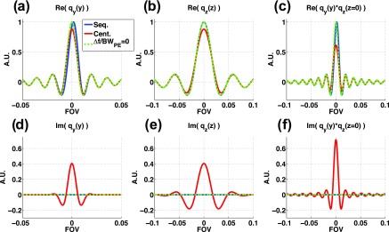
PSF distorted by a Gaussian shaped, temperature-induced, and spatially dependent phase term. (a)–(c) show the real parts of q_y(y), q_z(z), and q_y(y) * q_z(z), and (d)–(f) show corresponding imaginary parts, respectively. Centrically sampled schemes are the only schemes with any signal in the imaginary channel, and it is this imaginary part that reduces the phase shift at the focal spot center, resulting in the underestimated temperatures. It can be noted that the ESC scheme, which only applies centric sampling in the k_y direction, would only experience an imaginary part in q_y(y), whereas the NESC2-VD2 scheme will have imaginary parts in both q_y(y) and q_z(z).

IV. DISCUSSION AND CONCLUSIONS

Several interesting observations can be made from this study relating to the relative accuracy of MRI temperature measurements obtained using different sampling and subsampling strategies. Most of these observations apply to segmented EPI GRE PRF measurements, but a few generalizations can be made.

First, it was found that centric sampling that samples the k-space center with the last echo in the echo train results in a consistent and systematic underestimation of temperatures. This is true both as a function of time where the centric schemes underestimates the temperatures throughout the HIFU heating, and as a function of position, where larger errors are observed in the centrically sampled phase encode directions. It was expected that having TE closer to T2* would improve the accuracy and precision of temperature measurements. However, it was found that the temperature increase at the focal spot causes a local change in the resonant frequency, which combined with centric sampling result in phase shifts of opposite polarities for different parts of k-space. These phase shifts in turn result in spatially dependent, bidirectional position shifts in the reconstructed image, where the hottest voxels experience the largest position shift. The PSF analysis confirmed that phase shifts of opposite polarities that occur in centric sampling result in a “blurring” effect (i.e., bidirectional position shift resulting in an increased FWHM) in the real part of the phase encode directions. It further introduces a contribution in the imaginary channel, reducing the phase shift at the focal spot center, resulting in temperature underestimations. The ESC scheme (which centrically samples only in k_y) showed a slightly larger FWHM in the phase encode direction, while the NESC2-VD2 scheme (which centrically samples in both k_y and k_z) showed a significantly larger FWHM in both the phase and slice encode directions, both compared to sequentially and fully sampled data. Although the simulation observations are in agreement with the experimental results, it should be noted that the exact k_y/k_z phase encoding order of the centrically sampled schemes were not included in the PSF analysis, so any predicted temperature error is only qualitative. Also, we note that this blurring and temperature underestimation occur whether or not k-space subsampling is performed.

Second, the underestimation of temperatures observed in the EPI implementation of the NESC2-VD2 scheme is not seen in the non-EPI GRE implementation of a similar subsampling scheme, showing that in GRE implementations both variable and nonvariable density sampling can be applied without introducing any temperature underestimations. In this case, all data are sampled with the same echo time so no phase is introduced across k-space, and hence no distortion or blurring is seen. In this case, the PSF for the subsampling schemes and the “truth” will all be identical, and no imaginary parts will be introduced.

Third, the results also demonstrate that accurate temperature measurements can be achieved with sequentially sampled schemes (i.e., ESS, ESS-VD1, and NESS-VD2), with Fig. 4 showing maximum errors of the hottest voxel of less than 1 °C throughout the experiment. The spatial distribution of temperature errors in Fig. 5 for these schemes are also seen to be substantially smaller than for the centrically sampled schemes in all three orthogonal views. Sequential sampling leads to a unidirectional phase across k-space, resulting in a position shift only in one direction. Since the shift is temperature dependent, it is larger for the center of the focal spot and decreases in magnitude for parts that experience less heating, resulting in a slight distortion of the focal spot shape. It should be noted that the fully sampled “truth” also utilizes sequential phase encoding, and hence will experience the same distortion of the focal spot shape. This effect can also be seen in the PSF [Fig. 11(a)]. From the imaginary parts of the PSF it can further be seen that the sequentially sampled schemes will not have any contributions in this channel, confirming that the temperatures will be accurately measured. Figure 7 and the ANOVA tests demonstrate that the fully sampled “truth” and all sequentially sampled schemes do not experience any significantly difference in FWHM values in either the phase or slice encode directions.

The size of the above-mentioned position shifts for the sequentially sampled schemes is usually less than a voxel, and can be predicted from temperature rise, ETL, and ES as previously described. For ETL = 7, and ES = 1.58 ms (i.e., BW_PE = 90.4 Hz/pixel) as used for the ESS and ESS-VD1 schemes, it would take a temperature rise of approximately 70 °C at 3 T to shift the center of the focal spot by 1 voxel.

Fourth, it was also shown that schemes utilizing equally spaced and sequential sampling (i.e., ESS and ESS-VD1) have optimal echo shifting and minimal imaging artifacts, whereas schemes utilizing nonequally spaced sampling experience echo shifting nonlinearities resulting in increased image artifacts. Echo shifting for the NESS-VD2 scheme is, by design, nonlinear as the early and later phase-encode increments are larger than the central to accommodate variable sampling density in the k_y direction. Even though the central part of k-space is traversed relatively linearly, increased levels of ringing artifacts can be seen in the magnitude compared to corresponding images for the ESS and ESS-VD1 schemes. The centrically sampled schemes also traverse k-space nonlinearly in time by design, and hence experience increased artifact levels in the reconstructed magnitude images. This is especially true for the NESC2-VD2 scheme due to the imperfect echo shifting in the k_y direction. Further, since different k-space lines are sampled in each time-frame, the above described artifacts vary in time.

This time variation of image artifacts will also be present in the image phase, and is reflected in the standard deviation through time of temperatures measured in an unheated region. Theoretically, the lowest temperature standard deviation will be achieved when TE is close to T₂*.^52,57,58 This would favor centric sampling schemes that have the longest TE (20.4 and 22.1 ms for ESC and NESC2-VD2, respectively, vs 15.0 ms for the sequentially sampled schemes). This is the case for the ESC scheme that has the lowest standard deviation (0.03 °C). The NESC2-VD2 scheme has a slightly larger standard deviation similar to the ESS scheme (0.06 °C vs 0.07 °C), due to the imperfect echo shifting and hence increased artifact level. The NESS-VD2 scheme has the highest standard deviation (0.10 °C), resulting from a combination of sequential sampling (shorter TE) and nonlinear k-space traversal in time. That the subsampling schemes have lower standard deviation than the fully sampled “truth” can be explained by the fact that the TCR algorithm tends to smooth out variations in time.

To the extent that RF coils with multiple receive channels can be used, the five subsampling schemes described in this paper could also be reconstructed with parallel imaging approaches such as SENSE or GRAPPA.^42,45 However, the centrically sampled schemes would result in temperature underestimations also with parallel imaging reconstruction approaches. It should be noted that to use parallel imaging to achieve the same reduction factor as used in this paper, arrays composed of at least seven (but for practical considerations probably more) receive coils would be needed.

Finally, the challenge of reconstruction speed is a major issue for iterative reconstruction methods such as TCR, although it is less of an issue in model-based and parallel imaging approaches.^{26,38,40,44,46,47} A real-time TCR algorithm has been described,⁵⁹ in which the computation burden is reduced by only applying the TCR algorithm on a limited FOV. The limited FOV is achieved by cropping the image for TCR reconstruction in the directions in which k-space is fully sampled. Thus, the limited FOV TCR method would experience the largest speedup for the ESS scheme where both the k_x and k_z directions can be cropped. For large FOV applications, the real-time TCR algorithm could be applied over the focal spot where temperatures are changing rapidly, and a sliding window approach can be applied over the rest of the image where temperatures can be assumed to change more slowly.

The results presented have demonstrated some relative advantages and disadvantages of each of the sampling schemes with the general observation that the sequential sampling schemes are more accurate than centric schemes. Based on these results, it is unlikely that 2D centric subsampling methods like the NESC2-VD2 method, which is artifactual and underestimates focal spot temperatures, will find utility. The ESC method is less artifactual, but would still underestimate focal spot temperatures. For sequential sampling schemes, the results show that increased temperature measurement accuracy can be achieved by varying the sampling density in 2D (as in NESS-VD2), compared to 0D and 1D (as in ESS and ESS-VD1, respectively). The increased accuracy, however, is achieved at the expense of decreased image quality, due to nonoptimal echo shifting. Whether highest possible accuracy, as in NESS-VD2, or a trade-off between accuracy and image quality, as in ESS-VD1, is preferred is in most instances likely to be application specific. For certain complex anatomies, e.g., the brain, the image quality of EPI in general is likely too low, and some alternative high-resolution anatomical imaging is likely desirable, while the maximum accuracy is probably desirable from the temperature measurements. For other less complex anatomies or in multiparameter imaging, such as simultaneous PRF-T1 imaging,^60,61 using magnitude-based T1 measurements to monitor temperatures in adipose tissue, the general image quality of EPI might be deemed adequate and a trade-off between image quality and (PRF-) temperature accuracy might be more appropriate. Therefore, the general guidelines as to what sampling approach to use are likely application specific.

In summary, we have investigated five approaches of k-space subsampling in a 3D segmented EPI pulse sequence for large FOV temperature monitoring during HIFU. The results demonstrate that, when using pulse sequences with EPI readouts for fast data acquisition, sequential sampling in the phase encode directions should be used to avoid underestimation of temperatures. Variable density sampling can be implemented to improve temperature measurement accuracy, by sampling the center of k-space more frequently. However, considerations have to be given to nonuniform k-space increments, which can degrade image quality by nonoptimal echo shifting. It is further shown that non-EPI GRE pulse sequences are not as sensitive to different k-space sampling approaches, and variable density sampling can be successfully implemented. With the methods described in this paper, temperature monitoring over a 192 × 144 × 135 mm³ FOV with a temporal resolution of 3.6 s was achieved, using R = 7, while keeping the RMSE below 0.35 °C.

APPENDIX A: DETAILED DESCRIPTION OF THE FIVE SAMPLING SCHEMES

The ESS scheme fully samples the k_x and k_z directions, while evenly subsampling the k_y direction by acquiring n equally spaced readout lines in each EPI segment, where each segment contains N_y/ETL phase encode lines (N_y is the total number of phase encode steps). By varying n, different R-values can be achieved, and R is calculated as N_y/(ETL * n). In the current experiment, the matrix size for this scheme is 128 × 98 × 54, and an ETL of 7 and n of 2 are used (for a total of 108 echo trains per time-frame), so as to achieve a R_tot = 7. For n = 2, one echo train is sampled in each of the 54 k_z’s, before coming back and acquiring a second echo train in each k_z. This second echo train is shifted (N_y/ETL)/2 k_y's compared to the first echo train, so as to create the equally spaced sampling. In this scheme the echo train is applied sequentially from low to high k_y, so that the center segment of k-space is always sampled with the middle echo in the echo train.

The ESS-VD1 scheme applies the echo train in the same way as in the ESS scheme, i.e., sequentially from low to high k_y's with a constant step size of N_y/ETL. In order to more frequently sample the center of k-space, the subsampling density in the k_z direction is made variable while maintaining equally spaced sampling in the k_y direction and fully sampling the k_x direction. Because the sampling density only varies along the k_z direction and is kept constant along k_y, the middle k_z's will be sampled more frequently but the sampling density along k_y is constant within each k_z. In the current experiment, the matrix size and ETL are identical to the ESS case. The 54 k_z's are divided into 7 regions containing 8, 5, 8, 12, 8, 5, and 8 k_z’s, respectively, Fig. 12(a). In each of the 7 regions 7, 5, 14, 56, 14, 5, and 7 echo trains, respectively, are applied in each time-frame, for a total of 108 echo trains as in the ESS scheme. The reduction factors for the 7 regions are R = 16-14-8-3-8-14-16, respectively, for a R_tot = 7 just as in the other sampling schemes investigated.

FIG. 12.

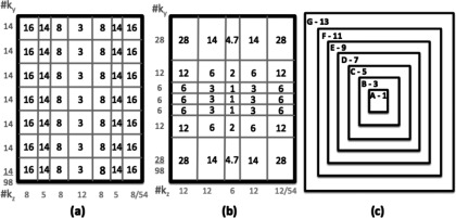
k_y-k_z plane for three of the subsampling schemes (Note: not drawn to scale). (a)–(b) ESS-VD1 and NESS-VD2, respectively. The number in each k-space region states what R was achieved in the corresponding region. Vertical/horizontal axis-labels state how many k_y's / k_z's belong to each of the regions, respectively. For (a) the sampling density varies along the k_z-direction but is constant along the k_y-direction, whereas for (b) the sampling density varies along both k_y and k_z. (c) The 7 2D regions (A–G, Table III) for the NESC2-VD2 scheme, with corresponding R’s, ranging from R = 1 for k-space center (region A) to R = 13 for the most peripheral parts (region G).

For the NESS-VD2 scheme variable density sampling in the k_z direction is achieved in the same fashion as for the ESS-VD1 scheme, by varying the number of echo trains applied over different regions in the k_z direction. To achieve variable density sampling in the second dimension (k_y), the phase encode “blips” are not constant within the echo train as in the ESS and ESS-VD1 schemes, but is instead larger for earlier and later echoes and smaller for the central echoes. The k_x direction is again fully sampled. In the current experiment, the matrix size and ETL for the NESS-VD2 scheme are the same as for the ESS and ESS-VD1 schemes. The 54 k_z's are divided into 5 regions containing 12, 12, 6, 12, and 12 k_z's, respectively, Fig. 12(b). In each of the 5 k_z-regions 12, 24, 36, 24, and 12 echo trains (for a total of 108), respectively, are applied in each time-frame. All echo trains in one k_z-region are applied before moving to the next region. The 7 k_y-segments of varying size contain 28, 12, 6, 6, 6, 12, 28 k_y's, respectively. The subsampling factor for each region in 2D can be found in Fig. 12(b), and R_tot = 7 as in the other schemes.

Like the ESS scheme, the ESC scheme fully samples the k_x and k_z directions, while evenly subsampling the k_y direction. However, the k_y direction is divided into N_y/(2 * ETL) segments where the lower half of the segments are sampled with positive phase encode “blips” and the upper half of the segments are sampled with negative phase encode “blips” to attain centric sampling. Adjusting how many echo trains are applied in each k_z can alter the subsampling factor, just like in the ESS scheme. In the current experiment the matrix size, ETL, and R_tot were the same as for the ESS scheme.

In the NESC2-VD2 scheme the k_y-k_z plane is divided into 2D regions, Fig. 12(c). The number of regions equals the ETL, and the echo trains are played out centrically in 2D so that the first echo only samples data in the outmost region, and the last echo in the echo train only samples data in the most central region. The number of echo trains played out in each dynamic time-frame is chosen so that the center most region is always fully sampled. By ensuring that the number of readout lines/region increases for each larger region, the reduction factor for each larger region will also be increasing. Each echo train is further constrained to only acquire data in one quadrant of the k_y-k_z plane, to minimize the amplitude of the phase encode “blips” and resulting eddy currents. The first echo train samples data in the first quadrant, and the corresponding lines are then sampled in the remaining three quadrants with the following three echo trains, giving rise to the symmetric appearance that can be observed in Fig. 1(e). In the current experiment, the matrix size was slightly different compared to the other sampling schemes, 128 × 126 × 42, but the same ETL of 7 was used. Hence, the k_y-k_z plane was divided into 7 regions. The sizes and R's of all regions are summarized in Table III. The same total number of echo trains per time-frame as for the other sampling schemes is used, 108 (27 in each quadrant of the k_y-k_z plane), and R_tot is the same, 7.

TABLE III.

Size, number of readout lines, and reduction factor for each of the 7 2D regions in Fig. 12(c). The number of readout lines in each region is the difference between its size and the size of the smaller region it surrounds. In the present case, 108 echo trains are applied in each time-frame, so, e.g., region E will have a reduction factor of R = 972/108 = 9. The total reduction factor will, for this matrix size and EPI factor, be R_tot = (126 × 42)/(7 × 108) = 7.

“Region”	Size (ky × kz)	# Readout lines	R
A	18 × 6	108	1
B	36 × 12	324	3
C	54 × 18	540	5
D	72 × 24	756	7
E	90 × 30	972	9
F	108 × 36	1188	11
G	126 × 42	1404	13
	Total:	5292	7

APPENDIX B: FULL DERIVATION OF THE POINT SPREAD FUNCTION

Derivation of Eqs. (2) and (3), the PSF distorted by a Gaussian shaped, temperature-induced, and spatially dependent phase term.

If relaxation terms and field inhomogeneities are ignored, the received MR signal for the jth phase encode, s_j, can be written as

$$s_j=\int M\left(y\right)e^{2\pi iyj\frac{\gamma }{2\pi }{G}_y\Delta t}dy,$$ (B1)

where M(y) is the magnetization density, G_y is the gradient strength, and Δt is the time increment between samples. Including a temperature induced spatially dependent phase term, Eq. (B1) becomes

$$s_j=\int M\left(y\right)e^{2\pi iyj\frac{\gamma }{2\pi }{G}_y\Delta t}{e}^{2\pi ij\frac{\gamma }{2\pi }\Delta B_T\Delta t}dy,$$ (B2)

where ΔB_T can be written as

$$\Delta B_T=B_0\Delta T\left(y\right)\alpha .$$ (B3)

Here ΔT(y) is the HIFU-induced spatially varying temperature rise, which in the current case is assumed to have a Gaussian shape with FWHM in conformity with Fig. 7 (7.5 mm in y, and 23.5 mm in z). From the discrete inverse Fourier transform, the reconstructed image can be obtained as

$$\begin{array}{ccc}\hfill M_r\left(y^{\prime }\right)& =& \frac{1}{N_y}\sum _{j=0}^{N_y-1}{s}_j{e}^{-2\pi i\frac{j{y}^{\prime }}{N_y\Delta y}}\hfill \\ & =& \frac{1}{N_y}\sum _{j=0}^{N_y-1}\int M\left(y\right)e^{2\pi iyj\frac{\gamma }{2\pi }{G}_y\Delta t}\hfill \\ & & \times e^{2\pi ij\frac{\gamma }{2\pi }\Delta B_T\Delta t}{e}^{-2\pi i\frac{j{y}^{\prime }}{N_y\Delta y}}dy,\hfill \end{array}$$ (B4)

where Δy is the voxel size, and N_y is the number of phase encode steps in the y-direction. Changing the summation limits over j to go from −(N-1)/2 to +(N-1)/2, and using the fact that Δt(N/2) = TE, Eq. (B4) can be written as

$$\begin{array}{ccc}\hfill M_r\left(y^{\prime }\right)& =& \frac{1}{N_y}\int M\left(y\right)e^{2\pi i\frac{\gamma }{2\pi }\Delta B_T\mathrm{TE}}\hfill \\ & & \times {\sum }_{j=-\frac{N_y-1}{2}}^{\frac{N_y-1}{2}}{e}^{2\pi ij\left(\frac{\gamma }{2\pi }\left[y{G}_y+\Delta B_T\right]\Delta t-\frac{y^{\prime }}{N_y\Delta y}\right)}dy.\hfill \end{array}$$ (B5)

Equation (B5) can be written in terms of the well-known function q(y, y′), as

$$|M_r\left(y^{\prime }\right)|e^{i\phi }=\int M\left(y\right)e^{2\pi i\frac{\gamma }{2\pi }\Delta B_T\mathrm{TE}}q\left(y,y^{\prime }\right)dy,$$ (B6)

where, using Δω = 2πΔf = ΔT(y)αB₀γ, q(y, y′) is

$$q_{\pm }\left(y,y^{\prime }\right)=\frac{1}{N_y}\sum e^{\frac{2\pi ij}{N_y}\left(\frac{y-y^{\prime }}{\Delta y}\pm \frac{\Delta f\left(y\right)}{{\mathrm{BE}}_{\mathrm{PE}}}\right)}.$$ (B7)

In Eq. (B7), the relationship G_yΔtγ/2π = 1/(N_yΔy) has been used. The term ±Δf(y)/BW_PE represents the polarity of the phase shift (i.e., if the data were acquired with positive (+) or negative (−) phase encode gradients). For the sequentially sampled schemes where all phase encode gradients are positive, Eq. (B7) becomes

$$q_{\mathrm{Seq}}\left(y,y^{\prime }\right)=\frac{1}{N_y}\left({\sum }_{j=-\frac{N_y-1}{2}}^{\frac{N_y-1}{2}}{e}^{\frac{2\pi ij}{N_y}\left(\frac{y-y^{\prime }}{\Delta y}+\frac{\Delta f\left(y\right)}{{\mathrm{BE}}_{\mathrm{PE}}}\right)}\right).$$ (B8)

In case of the centrically sampled schemes, where both positive and negative phase encode gradients are applied, the summation needs to be split into two parts representing lower and upper parts of k-space, respectively, and Eq. (B7) becomes

$$\begin{array}{ccc}\hfill q_{\mathrm{Cent}}\left(y,y^{\prime }\right)& =& \frac{1}{N_y}({\sum }_{j=-\frac{N_y-1}{2}}^{-\frac{1}{2}}{e}^{\frac{2\pi ij}{N_y}\left(\frac{y-y^{\prime }}{\Delta y}+\frac{\Delta f\left(y\right)}{{\mathrm{BE}}_{\mathrm{PE}}}\right)}\hfill \\ & & +{\sum }_{j=\frac{1}{2}}^{\frac{N_y-1}{2}}{e}^{\frac{2\pi ij}{N_y}\left(\frac{y-y^{\prime }}{\Delta y}-\frac{\Delta f\left(y\right)}{{\mathrm{BE}}_{\mathrm{PE}}}\right)}).\hfill \end{array}$$ (B9)

REFERENCES

- 1.Wu F.et al. , “Extracorporeal high intensity focused ultrasound ablation in the treatment of 1038 patients with solid carcinomas in China: An overview,” Ultrason. Sonochem. 11(3-4), 149–54 (2004). 10.1016/j.ultsonch.2004.01.011 [DOI] [PubMed] [Google Scholar]
- 2.Dromi S.et al. , “Pulsed-high intensity focused ultrasound and low temp-erature-sensitive liposomes for enhanced targeted drug delivery and antitumor effect,” Clin. cancer Res. 13(9), 2722–2727 (2007). 10.1158/1078-0432.CCR-06-2443 [DOI] [PMC free article] [PubMed] [Google Scholar]
- 3.Ferrara K., Pollard R., and Borden M., “Ultrasound microbubble contrast agents: Fundamentals and application to gene and drug delivery,” Annu. Rev. Biomed. Eng. 9, 415–47 (2007). 10.1146/annurev.bioeng.8.061505.095852 [DOI] [PubMed] [Google Scholar]
- 4.Mesiwala A.et al. , “High-intensity focused ultrasound selectively disrupts the blood-brain barrier in vivo,” Ultrasound Med. Biol. 28(3), 389–400 (2002). 10.1016/S0301-5629(01)00521-X [DOI] [PubMed] [Google Scholar]
- 5.Payne A.et al. , “Design and characterization of a laterally mounted phased-array transducer breast-specific MRgHIFU device with integrated 11-channel receiver array,” Med. Phys. 39(3), 1552–1560 (2012). 10.1118/1.3685576 [DOI] [PMC free article] [PubMed] [Google Scholar]
- 6.Hynynen K.et al. , “MR imaging-guided focused ultrasound surgery of fibroadenomas in the breast: A feasibility study,” Radiology 219(1), 176–185 (2001). 10.1148/radiology.219.1.r01ap02176 [DOI] [PubMed] [Google Scholar]
- 7.Huber P. E.et al. , “A new noninvasive approach in breast cancer therapy using magnetic resonance imaging-guided focused ultrasound surgery,” Cancer Res. 61, 8441–8447 (2001). [PubMed] [Google Scholar]
- 8.Ries M., Denis de Senneville B., Roujol S., Berber Y., Quesson B., and Moonen C., “Real-time 3D target tracking in MRI guided focused ultrasound ablations in moving tissues,” Magn. Reson. Med. 64(6), 1704–1712 (2010). 10.1002/mrm.22548 [DOI] [PubMed] [Google Scholar]
- 9.Quesson B.et al. , “A method for MRI guidance of intercostal high intensity focused ultrasound ablation in the liver,” Med. Phys. 37(6), 2533–2540 (2010). 10.1118/1.3413996 [DOI] [PubMed] [Google Scholar]
- 10.Daum D. R., Smith N. B., King R., and Hynynen K., “In vivo demonstration of noninvasive thermal surgery of the liver and kidney using an ultrasonic phased array,” Ultrasound Med. Biol. 25(7), 1087–1098 (1999). 10.1016/S0301-5629(99)00053-8 [DOI] [PubMed] [Google Scholar]
- 11.Salomir R.et al. , “Local delivery of magnetic resonance (MR) contrast agent in kidney using thermosensitive liposomes and MR imaging-guided local hyperthermia: A feasibility study in vivo,” J. Magn. Reson. imaging 22(4), 534–540 (2005). 10.1002/jmri.20416 [DOI] [PubMed] [Google Scholar]
- 12.Denis de Senneville B., Mougenot C., and Moonen C. T. W., “Real-time adaptive methods for treatment of mobile organs by MRI-controlled high-intensity focused ultrasound,” Magn. Reson. Med. 57(2), 319–330 (2007). 10.1002/mrm.21124 [DOI] [PubMed] [Google Scholar]
- 13.Diederich C. J., Stafford R. J., Nau W. H., Burdette E. C., Price R. E., and Hazle J. D., “Transurethral ultrasound applicators with directional heating patterns for prostate thermal therapy: In vivo evaluation using magnetic resonance thermometry,” Med. Phys. 31(2), 405–413 (2004). 10.1118/1.1639959 [DOI] [PubMed] [Google Scholar]
- 14.Chopra R.et al. , “MRI-compatible transurethral ultrasound system for the treatment of localized prostate cancer using rotational control,” Med. Phys. 35(4), 1346–1357 (2008). 10.1118/1.2841937 [DOI] [PubMed] [Google Scholar]
- 15.McDannold N., Tempany C. M., Fennessy F. M., Stewart E. A., and Jolesz F. A., “Uterine leiomyomas: MR imaging-based thermometry and thermal dosimetry during focused ultrasound thermal ablation,” Radiology 240(1), 263–272 (2006). 10.1148/radiol.2401050717 [DOI] [PMC free article] [PubMed] [Google Scholar]
- 16.Hynynen K.et al. , “Pre-clinical testing of a phased array ultrasound system for MRI-guided noninvasive surgery of the brain: A primate study,” Eur. J. Radiol. 59(2), 149–156 (2006). 10.1016/j.ejrad.2006.04.007 [DOI] [PubMed] [Google Scholar]
- 17.McDannold N., Clement G., Black P., Jolesz F., and Hynynen K., “Transcranial MRI-guided focused ultrasound surgery of brain tumors: Initial findings in three patients,” Neurosurgery 66(2), 323–332 (2010). 10.1227/01.NEU.0000360379.95800.2F [DOI] [PMC free article] [PubMed] [Google Scholar]
- 18.Monteith S. J.et al. , “Transcranial magnetic resonance-guided focused ultrasound surgery for trigeminal neuralgia: A cadaveric and laboratory feasibility study,” J. Neurosurg. 118(2), 319–328 (2013). 10.3171/2012.10.JNS12186 [DOI] [PubMed] [Google Scholar]
- 19.Jeanmonod D.et al. , “Transcranial magnetic resonance imaging-guided focused ultrasound: Noninvasive central lateral thalamotomy for chronic neuropathic pain,” Neurosurg. Focus 32(1), 1–11 (2012). 10.3171/2011.10.FOCUS11248 [DOI] [PubMed] [Google Scholar]
- 20.Payne A., Vyas U., Todd N., de Bever J., Christensen D. A., and Parker D. L., “The effect of electronically steering a phased array ultrasound transducer on near-field tissue heating,” Med. Phys. 38(9), 4971–4981 (2011). 10.1118/1.3618729 [DOI] [PMC free article] [PubMed] [Google Scholar]
- 21.Mougenot C., Köhler M. O., Enholm J., Quesson B., and Moonen C., “Quantification of near-field heating during volumetric MR-HIFU ablation,” Med. Phys. 38(1), 272–282 (2011). 10.1118/1.3518083 [DOI] [PubMed] [Google Scholar]
- 22.Connor C. W. and Hynynen K., “Patterns of thermal deposition in the skull during transcranial focused ultrasound surgery,” IEEE Trans. Biomed. Eng. 51(10), 1693–706 (2004). 10.1109/TBME.2004.831516 [DOI] [PubMed] [Google Scholar]
- 23.Weidensteiner C.et al. , “Real-time MR temperature mapping of rabbit liver in vivo during thermal ablation,” Magn. Reson. Med. 50(2), 322–330 (2003). 10.1002/mrm.10521 [DOI] [PubMed] [Google Scholar]
- 24.Stafford R. J., Price R. E., Diederich C. J., Kangasniemi M., Olsson L. E., and Hazle J. D., “Interleaved echo-planar imaging for fast multiplanar magnetic resonance temperature imaging of ultrasound thermal ablation therapy,” J. Magn. Reson. imaging 20(4), 706–714 (2004). 10.1002/jmri.20157 [DOI] [PubMed] [Google Scholar]
- 25.Cernicanu A., Lepetit-Coiffe M., Roland J., Becker C. D., and Terraz S., “Validation of fast MR thermometry at 1.5 T with gradient-echo echo planar imaging sequences: Phantom and clinical feasibility studies,” NMR Biomed. 21, 849–858 (2008). 10.1002/nbm.1267 [DOI] [PubMed] [Google Scholar]
- 26.Denis de Senneville B., Roujol E., Hey S., Moonen C., and Ries M., “Extended Kalman filtering for continuous volumetric MR-temperature imaging,” IEEE Trans. Med. Imaging 32(4), 711–718 (2013). 10.1109/TMI.2012.2234760 [DOI] [PubMed] [Google Scholar]
- 27.Roujol S., Ries M., Quesson B., Moonen C., and Denis de Senneville B., “Real-time MR-thermometry and dosimetry for interventional guidance on abdominal organs,” Magn. Reson. Med. 63(4), 1080–1087 (2010). 10.1002/mrm.22309 [DOI] [PubMed] [Google Scholar]
- 28.Kickhefel A., Roland J., Weiss C., and Schick F., “Accuracy of real-time MR temperature mapping in the brain: A comparison of fast sequences,” Phys. Med. 26(4), 192–201 (2010). 10.1016/j.ejmp.2009.11.006 [DOI] [PubMed] [Google Scholar]
- 29.van Vaals J. J.et al. , “‘Keyhole’ method for accelerating imaging of contrast agent uptake,” J. Magn. Reson. imaging 3(4), 671–675 (1993). 10.1002/jmri.1880030419 [DOI] [PubMed] [Google Scholar]
- 30.Doyle M., Walsh E. G., Blackwell G. G., and Pohost G. M., “Block regional interpolation scheme for k-space (BRISK): A rapid cardiac imaging technique,” Magn. Reson. Med. 33(2), 163–170 (1995). 10.1002/mrm.1910330204 [DOI] [PubMed] [Google Scholar]
- 31.Parrish T. and Hu X., “Continuous update with random encoding (CURE): A new strategy for dynamic imaging,” Magn. Reson. Med. 33(3), 326–336 (1995). 10.1002/mrm.1910330307 [DOI] [PubMed] [Google Scholar]
- 32.Korosec F. R., Frayne R., Grist T. M., and Mistretta C. A., “Time-resolved contrast-enhanced 3D MR angiography,” Magn. Reson. Med. 36(3), 345–351 (1996). 10.1002/mrm.1910360304 [DOI] [PubMed] [Google Scholar]
- 33.Saranathan M., Rettmann D., Bayram E., Lee C., and Glockner J., “Multiecho time-resolved acquisition (META): A high spatiotemporal resolution Dixon imaging sequence for dynamic contrast-enhanced MRI,” J. Magn. Reson. Imaging 29(6), 1406–1413 (2009). 10.1002/jmri.21750 [DOI] [PubMed] [Google Scholar]
- 34.Madhuranthakam A. J.et al. , “Undersampled elliptical centric view-order for improved spatial resolution in contrast-enhanced MR angiography,” Magn. Reson. Med. 55(1), 50–58 (2006). 10.1002/mrm.20726 [DOI] [PubMed] [Google Scholar]
- 35.Vogt F. M.et al. , “High spatial and temporal resolution MRA (TWIST) in acute aortic dissection,” Proc. Int. Soc. Magn. Reson. Med. 15, 92 (2007). [Google Scholar]
- 36.Song T.et al. , “Optimal k-space sampling for dynamic contrast-enhanced MRI with an application to MR renography,” Magn. Reson. Med. 61(5), 1242–1248 (2009). 10.1002/mrm.21901 [DOI] [PMC free article] [PubMed] [Google Scholar]
- 37.Saranathan M., Rettmann D. W., Hargreaves B. A., Clarke S. E., and Vasanawala S. S., “DIfferential Subsampling with Cartesian Ordering (DISCO): A high spatio-temporal resolution Dixon imaging sequence for multiphasic contrast enhanced abdominal imaging,” J. Magn. Reson. imaging 35(6), 1484–1492 (2012). 10.1002/jmri.23602 [DOI] [PMC free article] [PubMed] [Google Scholar]
- 38.Huang F., Köhler M., Tanttu J., Deckers R., Lin W., and Duensing G. R., “A clinically applicable approach for higher spatiotemporal resolution thermometry mapping,” Proc. Int. Soc. Magn. Reson. Med. 20, 561 (2012). [Google Scholar]
- 39.Todd N., Adluru G., Payne A., DiBella E. V. R., and Parker D., “Temporally constrained reconstruction applied to MRI temperature data,” Magn. Reson. Med. 62(2), 406–419 (2009). 10.1002/mrm.22012 [DOI] [PMC free article] [PubMed] [Google Scholar]
- 40.Todd N., Payne A., and Parker D. L., “Model predictive filtering for improved temporal resolution in MRI temperature imaging,” Magn. Reson. Med. 63(5), 1269–1279 (2010). 10.1002/mrm.22321 [DOI] [PMC free article] [PubMed] [Google Scholar]
- 41.Todd N., Vyas U., de Bever J., Payne A., and Parker D. L., “Reconstruction of fully three-dimensional high spatial and temporal resolution MR temperature maps for retrospective applications,” Magn. Reson. Med. 67(3), 724–730 (2012). 10.1002/mrm.23055 [DOI] [PMC free article] [PubMed] [Google Scholar]
- 42.Griswold M. A.et al. , “Generalized autocalibrating partially parallel acquisitions (GRAPPA),” Magn. Reson. Med. 47(6), 1202–1210 (2002). 10.1002/mrm.10171 [DOI] [PubMed] [Google Scholar]
- 43.Huang F., Akao J., Vijayakumar S., Duensing G. R., and Limkeman M., “k-t GRAPPA: A k-space implementation for dynamic MRI with high reduction factor,” Magn. Reson. Med. 54(5), 1172–1784 (2005). 10.1002/mrm.20641 [DOI] [PubMed] [Google Scholar]
- 44.Guo J. Y., Kholmovski E. G., Zhang L., Jeong E.-K., and Parker D. L., “k-space inherited parallel acquisition (KIPA): Application on dynamic magnetic resonance imaging thermometry,” Magn. Reson. Imaging 24(7), 903–915 (2006). 10.1016/j.mri.2006.03.001 [DOI] [PubMed] [Google Scholar]
- 45.Pruessmann K. P., Weiger M., Scheidegger M. B., and Boesiger P., “SENSE: Sensitivity encoding for fast MRI,” Magn. Reson. Med. 42(5), 952–962 (1999). [DOI] [PubMed] [Google Scholar]
- 46.Weidensteiner C., Kerioui N., Quesson B., Denis de Senneville B., Trillaud H., and Moonen C. T. W., “Stability of real-time MR temperature mapping in healthy and diseased human liver,” J. Magn. Reson. Imaging 19(4), 438–446 (2004). 10.1002/jmri.20019 [DOI] [PubMed] [Google Scholar]
- 47.Mei C. S.et al. , “Combining two-dimensional spatially selective RF excitation, parallel imaging, and UNFOLD for accelerated MR thermometry imaging,” Magn. Reson. Med. 66(1), 112–122 (2011). 10.1002/mrm.22788 [DOI] [PMC free article] [PubMed] [Google Scholar]
- 48.Pennes H. H., “Analysis of tissue and arterial blood temperatures in the resting human forearm,” J. Appl. Physiol. 1(2), 93–122 (1948). [DOI] [PubMed] [Google Scholar]
- 49.Marx M. and Butts Pauly K., “Use of compressed sensing for acceleration of volumetric MR thermometry,” in 9th International Interventional MRI Symposium (Boston, 2012), p. 110 [Google Scholar]
- 50.Ishihara Y., Calderon A., Watanabe H., Okamoto K., Suzuki Y., and Kuroda K., “A precise and fast temperature mapping using water proton chemical shift,” Magn. Reson. Med. 34(6), 814–823 (1995). 10.1002/mrm.1910340606 [DOI] [PubMed] [Google Scholar]
- 51.Bernstein M. A., King K. F., and Zhou X. J., Handbook of MRI Pulse Sequences (Elsevier, London, 2004). [Google Scholar]
- 52.Quesson B., de Zwart J. A., and Moonen C. T., “Magnetic resonance temperature imaging for guidance of thermotherapy,” J. Magn. Reson. Imaging 12(4), 525–533 (2000). [DOI] [PubMed] [Google Scholar]
- 53.Adluru G., Awate S. P., Tasdizen T., Whitaker R. T., and Dibella E. V. R., “Temporally constrained reconstruction of dynamic cardiac perfusion MRI,” Magn. Reson. Med. 57(6), 1027–1036 (2007). 10.1002/mrm.21248 [DOI] [PubMed] [Google Scholar]
- 54.Hayes C. E., Mathis C. M., and Yuan C., “Surface coil phased arrays for high-resolution imaging of the carotid arteries,” J. Magn. Reson. Imaging 6(1), 109–112 (1996). 10.1002/jmri.1880060121 [DOI] [PubMed] [Google Scholar]
- 55.Parker D. L., Du Y. P., and Davis W. L., “The voxel sensitivity function in Fourier transform imaging: Applications to magnetic resonance angiography,” Magn. Reson. Med. 33(2), 156–162 (1995). 10.1002/mrm.1910330203 [DOI] [PubMed] [Google Scholar]
- 56.Haacke E. M., Brown R. W., Thompson M. R., and Venkatesan R., Magnetic Resonance Imaging: Physical Principles and Sequence Design (John Wiley & Sons, New York, 1999). [Google Scholar]
- 57.Kuroda K.et al. , “Temperature mapping using the water proton chemical shift: Self-referenced method with echo-planar spectroscopic imaging,” Magn. Reson. Med. 43(2), 220–225 (2000). [DOI] [PubMed] [Google Scholar]
- 58.Cline H. E.et al. , “Simultaneous magnetic resonance phase and magnitude temperature maps in muscle,” Magn. Reson. Med. 35(3), 309–315 (1996). 10.1002/mrm.1910350307 [DOI] [PubMed] [Google Scholar]
- 59.Todd N.et al. , “Toward real-time availability of 3D temperature maps created with temporally constrained reconstruction,” Magn. Reson. Med. 71(4), 1394–404 (2014). 10.1002/mrm.24783 [DOI] [PMC free article] [PubMed] [Google Scholar]
- 60.Hey S.et al. , “Simultaneous T1 measurements and proton resonance frequency shift based thermometry using variable flip angles,” Magn. Reson. Med. 67(2), 457–463 (2012). 10.1002/mrm.22987 [DOI] [PubMed] [Google Scholar]
- 61.Todd N., Diakite M., Payne A., and Parker D. L., “Hybrid proton resonance frequency/T1 technique for simultaneous temperature monitoring in adipose and aqueous tissues,” Magn. Reson. Med. 69(1), 62–70 (2013). 10.1002/mrm.24228 [DOI] [PMC free article] [PubMed] [Google Scholar]