Two-dimensional segmentation for analyzing Hi-C data

Abstract

Motivation: The spatial conformation of the chromosome has a deep influence on gene regulation and expression. Hi-C technology allows the evaluation of the spatial proximity between any pair of loci along the genome. It results in a data matrix where blocks corresponding to (self-)interacting regions appear. The delimitation of such blocks is critical to better understand the spatial organization of the chromatin. From a computational point of view, it results in a 2D segmentation problem.

Results: We focus on the detection of cis-interacting regions, which appear to be prominent in observed data. We define a block-wise segmentation model for the detection of such regions. We prove that the maximization of the likelihood with respect to the block boundaries can be rephrased in terms of a 1D segmentation problem, for which the standard dynamic programming applies. The performance of the proposed methods is assessed by a simulation study on both synthetic and resampled data. A comparative study on public data shows good concordance with biologically confirmed regions.

Availability and implementation: The HiCseg R package is available from the Comprehensive R Archive Network and from the Web page of the corresponding author.

Contact: celine.levy-leduc@agroparistech.fr

1 INTRODUCTION

Many key steps of the cell development and cycle, such as DNA replication and gene expression are influenced by the 3D structure of the chromatin (Dixon et al., 2012). The folding of the chromosome in the space defines chromosomal territories, the function of which has been studied for few years now (Lieberman-Aiden et al., 2009). Typically, topologically associating domains contain clusters of genes that are co-regulated (Nora et al., 2012). Thus, the detection of chromosomal regions having close spatial location in the nucleus will provide insights for a better understanding of the influence of the chromosomal conformation on the cells functioning.

Several chromosome conformation capture technologies have been developed in the past decade, among which Hi-C is the most recent. This technology is based on a deep sequencing approach and provides read pairs corresponding to pairs of genomic loci that physically interact in the nucleus (Lieberman-Aiden et al., 2009). The raw measurement provided by Hi-C is therefore a list of pairs of locations along the chromosome, at the nucleotide resolution. These measurement are often summarized as a square matrix Y, where Y_i,j stands for the total number of read pairs matching in position i and position j, respectively. Positions refer here to a sequence of non-overlapping windows of equal sizes covering the genome. The number n of windows may vary from one study to another: Lieberman-Aiden et al. (2009) considered an Mb resolution, whereas Dixon et al. (2012) went deeper and used windows of 100 kb.

Blocks of higher intensity arise among this matrix, revealing both cis- and trans-interacting regions (Fraser et al., 2009). Although both types of interaction are likely to exist, cis-interacting regions seem to be prominent in the data (see Dixon et al., 2012, and Figs 7 and 8, for instance), and some have been confirmed to host co-regulated genes (Nora et al., 2012). Such regions result in block of higher signal along the diagonal of the data matrix. The purpose of the statistical analysis is then to provide a fully automated and efficient strategy to determine these regions. A first attempt was presented in Dixon et al. (2012), where the author strategy is first to summarize the 2D data into a 1D index, called the directionality index, then to apply a regular hidden Markov model to the summary data to retrieve the segmentation.

Fig. 7.

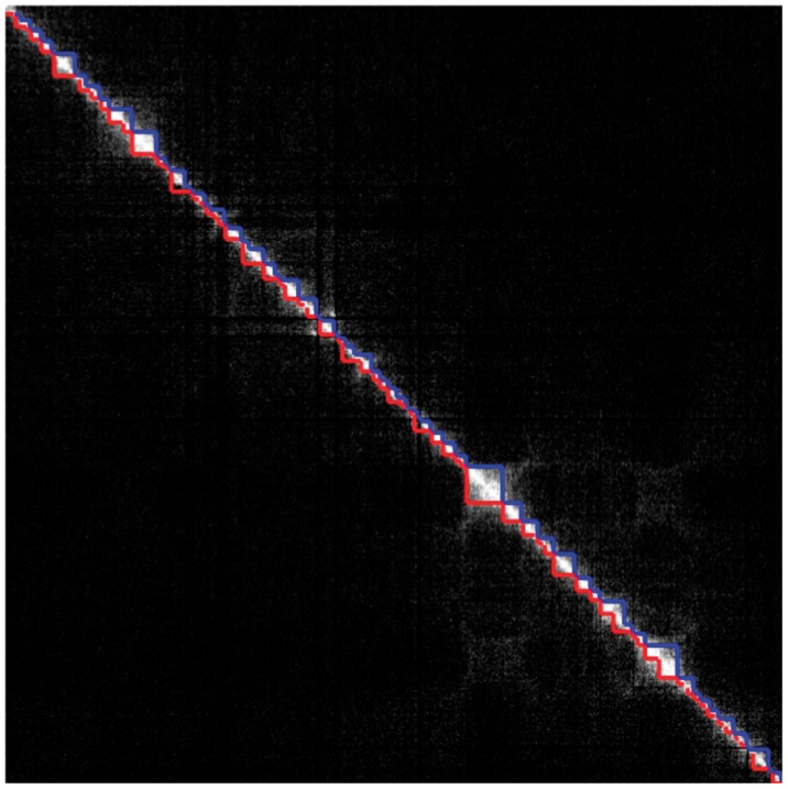
Topological domains detected by Dixon et al. (2012) (lower triangular part of the matrix) and by our method (upper triangular part of the matrix) from the interaction matrix of Chromosome 17 of the hESCs using Model (5) (P)

Fig. 8.

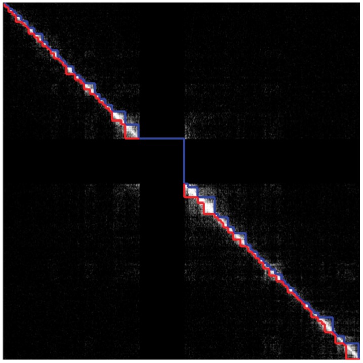
Topological domains detected by Dixon et al. (2012) (lower triangular part of the matrix) and by our method (upper triangular part of the matrix) from the interaction matrix of Chromosome 19 of the hESCs using Model (5) (P)

In this article, we show that such a two-step strategy can be avoided, and that summarizing the data is not required to solve the segmentation problem. Detecting diagonal blocks can be seen as a particular 2D segmentation issue. The 2D segmentation has been widely investigated for the detection of contour with arbitrary shape in images (see, for example, Darbon and Sigelle, 2006a, b; Hochbaum, 2001). From a computational point of view, image segmentation is an open problem because no predefined ordering exists that could be used to provide exact and efficient algorithms. Compared with contour detection, it is worth noticing that Hi-C data segmentation displays a specific pattern that did not receive any special attention from the image processing community. One of our contributions is to prove that this 2D segmentation problem boils down to a 1D segmentation problem for which efficient dynamic programming algorithms apply (Bellman, 1961; Lavielle, 2005; Picard et al., 2005). Our formulation of the problem also allows us to solve some non-block diagonal segmentation problems (see the end of Section 2.2).

The article is organized as follows. In Section 2, we define a general statistical model for Hi-C data, which can deal with both raw and normalized data. We prove that the maximum likelihood estimates of the block boundaries can be efficiently retrieved. In Section 3, we first present an extensive simulation study to assess the performance of our approach on both simulated and resampled data. We then apply the proposed methodology to the data studied by Dixon et al. (2012), which are publicly available, and compare our results with their regions. The package implementing the proposed method is presented in Section 4 where some open problems are also discussed.

2 STATISTICAL FRAMEWORK

2.1 Statistical modeling

We first define our statistical model. Because the Hi-C data matrix is symmetric, we only consider its upper triangular part denoted by Y, in which $Y_{i,j}(1\le i\le j\le n)$ stands for the intensity of the interaction between positions i and j. We suppose that all intensities are independent random variables with distribution

$$Y_{i,j}\sim p(·;{\mu }_{i,j}),{\mu }_{i,j}=\mathbb{E}(Y_{i,j})$$ (1)

where the matrix of means ${({\mu }_{i,j})}_{1\le i\le j\le n}$ is an upper triangular block diagonal matrix. An example of such a matrix is displayed in Figure 1 (left). Namely, we define the (half) diagonal blocks $D_k^{\mathrm{\star }}(k=1,\dots K^{\mathrm{\star }})$ as

$$D_k^{\mathrm{\star }}=\{(i,j):t_{k-1}^{\mathrm{\star }}\le i\le j\le t_k^{\mathrm{\star }}-1\}$$ (2)

where $1=t_0^{\mathrm{\star }}<t_1^{\mathrm{\star }}<\cdots <t_{K^{\mathrm{\star }}}^{\mathrm{\star }}=n+1$ stand for the true block boundaries and $K^{\mathrm{\star }}$ for the true number of blocks. We further define $E_0^{\mathrm{\star }}$ as the set of positions lying outside these blocks:

$$E_0^{\mathrm{\star }}=\{(i,j):1\le i\le j\le n\}\cap \overline{\left(\cup D_k^{\mathrm{\star }}\right)},$$ (3)

where $\overline{A}$ denotes the complement of the set A. The parameters $({\mu }_{i,j})$ are then supposed to be block-wise constant:

$$\begin{array}{c}{\mu }_{i,j}={\mu }_k^{\mathrm{\star }}\text{if}(i,j)\in D_k^{\mathrm{\star }},k=1,\dots ,K^{\mathrm{\star }},\\ ={\mu }_0^{\mathrm{\star }}\text{if}(i,j)\in E_0^{\mathrm{\star }}.\end{array}$$ (4)

Fig. 1.

Examples of block diagonal and extended block diagonal matrices ${({\mu }_{i,j})}_{1\le i\le j\le n}$. Left: Model (4), right: Model (9)

As for the distribution $p(·;{\mu }_{i,j})$ defined in (1), we will consider Gaussian, Poisson or negative binomial distributions:

$$\begin{array}{l}(\text{G}):Y_{i,j}\sim \mathcal{N}({\mu }_{i,j},{\sigma }^2),\\ (\text{P}):Y_{i,j}\sim \mathcal{P}({\mu }_{i,j}),\\ (\text{B}):Y_{i,j}\sim \mathcal{N}\mathcal{B}({\mu }_{i,j},\varphi ).\end{array}$$ (5)

The Gaussian modeling (G) will be typically used for dealing with normalized Hi-C data and the others [(P) and (B)] to deal with raw Hi-C data, which are count data. In Models (G) and (B), note that the parameters σ and ϕ are assumed to be constant and depend neither on i nor on j.

2.2 Inference

We now consider the estimation of the block boundaries ${(t_k^{\mathrm{\star }})}_{0\le k\le K^{\mathrm{\star }}}$ in the case where the number of blocks $K^{\mathrm{\star }}$ is known. Model selection issues will be discussed in Section 2.3. We consider a maximum likelihood approach. For an arbitrary set of blocks D_k, with boundaries ${(t_k)}_{0\le k\le K}$ and parameters ${({\mu }_k)}_{0\le k\le K}$, the log-likelihood of the data satisfying (1) and (4) writes

$$\begin{array}{c}\ell (Y)={\displaystyle \sum _{1\le i\le j\le n}\log }p(Y_{i,j};{\mu }_{ij})\\ ={\displaystyle \sum _{k=1}^K{\displaystyle \sum _{(i,j)\in D_k}\log }}p(Y_{i,j};{\mu }_k)+{\displaystyle \sum _{(i,j)\in E_0}\log }p(Y_{i,j};{\mu }_0),\end{array}$$

where D_k and E₀ are defined as in (2) and (3), respectively, except that the $t_k^{\mathrm{\star }}$s are replaced by the t_ks.

Parameter estimation

For given boundaries $t_0,\dots ,t_K$, the estimation of the block parameters μ_k is straightforward for each of the distribution considered in (5). Denoting ${\ell }_k(Y_{i,j})$ and ${\ell }_0(Y_{i,j})$ the contribution of each data point to the log-likelihood (up to some constants), in D_k and E_0, respectively, we get, for known parameters ϕ and μ₀,

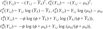where ${\overline{Y}}_k={\displaystyle {\sum }_{(i,j)\in D_k}{Y}_{i,j}}/|D_k|$, for k in $\{1,\dots ,K\},|A|$ denoting the cardinality of the set A.

Dynamic programming algorithm

Let us now consider the estimation of the boundaries $t_0,\dots t_K$. The objective function can be rewritten as follows:

$$\begin{array}{c}\ell (Y)={\displaystyle \sum _{k=1}^K{\displaystyle \sum _{(i,j)\in D_k}{\ell }_k}}(Y_{i,j})+{\displaystyle \sum _{(i,j)\in E_0}{\ell }_0}(Y_{i,j})\\ ={\displaystyle \sum _{k=1}^K\left({\displaystyle \sum _{(i,j)\in D_k}{\ell }_k}(Y_{i,j})+{\displaystyle \sum _{(i,j)\in R_k}{\ell }_0}(Y_{i,j})\right)}\end{array}$$

where R_k corresponds to the rectangle above D_k (see Fig. 1), namely, $R_k=\{(i,j):t_{k-1}\le j\le t_k-1,1\le i\le t_{k-1}-1\}$. (Note that R₁ is empty.) Note that the rectangles R_k do not overlap and that $E_0={\displaystyle \underset{k}{\cup }{R}_k}$, so the last equality holds. The important point here is that the objective function is now additive with respect to the successive intervals $\{t_{k-1},\dots t_k-1\},1\le k\le K$.

Defining the gain function

$$C(t_{k-1},t_k-1)={\displaystyle \sum _{(i,j)\in D_k}{\ell }_k}(Y_{i,j})+{\displaystyle \sum _{(i,j)\in R_k}{\ell }_0}(Y_{i,j}),$$ (6)

we have to maximize w.r.t. $1=t_0<t_1<\dots <t_K=n+1$

$${\displaystyle \sum _{k=1}^{K}C}(t_{k-1},t_k-1),$$

which can be done using the standard dynamic programming recursion (Bellman, 1961). For any $1\le L\le K$ and $1<\tau \le n$, we define

$$I_L(\tau )=\underset{1=t_0<t_1<\cdots <t_L=\tau +1}{\max }{\displaystyle \sum _{k=1}^{L}C}(t_{k-1},t_k-1)$$

the value of the objective function for the optimal segmentation of the submatrix made of the first τ rows and columns of Y into L blocks. Clearly, we have $I_1(\tau )=C(1,\tau )$,

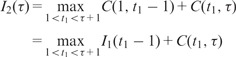and, for $3\le L\le K$,

$$I_L(\tau )=\underset{1<t_{L-1}<\tau +1}{\max }{I}_{L-1}(t_{L-1}-1)+C(t_{L-1},\tau ).$$ (7)

Hence, the optimal segmentation can be recovered with complexity $O(K{n}^2)$, once the $C(·,·)$ have been computed.

Common parameters

The optimization procedure described above applies when both ${\mu }_0$ and ϕ are known. Estimates of these parameters can be obtained in the following way. The estimate ${\widehat{\mu }}_0$ of μ₀ can be computed as the empirical mean of the observations lying in the right upper corner of the matrix Y, for instance,

$$T_0=\{(i,j):1\le i\le n/4,(3n/4+1)\le j\le n\}.$$ (8)

As for the overdispersion parameter of the negative binomial distribution ϕ, we computed $\widehat{\varphi }$ as follows: $\widehat{\varphi }={\widehat{\mu }}_0^2/({\widehat{\sigma }}_0^2-{\widehat{\mu }}_0),$ where ${\widehat{\sigma }}_0^2$ corresponds to the empirical variance of the observations lying in the same right upper corner of the matrix Y as for ${\widehat{\mu }}_0$.

Non-block diagonal segmentation problem

Observe that a similar procedure could be used for dealing with a more general matrix ${({\mu }_{i,j})}_{1\le i\le j\le n}$ defined by

$$\begin{array}{c}{\mu }_{i,j}={\mu }_k^{\mathrm{\star }}\text{if}(i,j)\in D_k^{\mathrm{\star }},k=1,\dots ,K^{\mathrm{\star }},\\ =\mu {\prime }_k{}^{\mathrm{\star }}\text{if}(i,j)\in R_k^{\mathrm{\star }},k=2,\dots ,K^{\mathrm{\star }},\end{array}$$ (9)

where the diagonal blocks $D_k^{\mathrm{\star }}$ and the rectangles $R_k^{\mathrm{\star }}$ are defined as above (see Fig. 1, right). In this case, no prior estimation of any mean parameter is required, as each $\mu {\prime }_k{}^{\mathrm{\star }}$ is specific to one single rectangle.

2.3 Model selection issue

In the case where the value of $K^{\mathrm{\star }}$ in the model defined by (1) and (4) is known a priori ${({\widehat{t}}_k)}_{1\le k\le K^{\mathrm{\star }}}$ can be obtained from the recursion (7), which actually gives the values of ${({\widehat{t}}_k)}_{1\le k\le K}$ for all $1\le K\le K_{max}$, where K_max is a given upper bound for the number of blocks. If $K^{\mathrm{\star }}$ is unknown, it can be estimated by $\widehat{K}$ defined as follows:

$$\widehat{K}={\text{Argmax}}_{1\le K\le K_{max}}{I}_K(n).$$ (10)

This strategy is illustrated in the next section.

3 RESULTS

Dixon et al. (2012) studied intrachromosomal interaction matrices for various chromosomes in both the human genome and the mouse genome at different resolutions (20 and 40 kb) and identified topological domains for each analyzed chromosome. Both the data and the topological domains found by Dixon et al. (2012) are available from the following Web page http://chromosome.sdsc.edu/mouse/hi-c/download.html. We worked on the same data, at a resolution 40 kb, to study the performance of our approach described above.

3.1 Application to synthetic data

We conducted several Monte Carlo simulations first on synthetic data and then on resampled real data to assess the sensibility of our method to block size and signal-to-noise ratio. The synthetic data are generated by using the domains found by Dixon et al. (2012) for Chromosome 19 of the cortex mouse. As for the resampled data, they are generated by using the Hi-C data of the chromosomes of the human embryonic stem cells (hESCs) provided by Dixon et al. (2012). The different simulation strategies are further described hereafter.

3.1.1 Fixed block design

To evaluate the performance of our methodology in the negative binomial framework, we generated block diagonal matrices according to Model (5) (B) where $({\mu }_{i,j})$ is defined by (4). More precisely, we generated 50 block diagonal interaction matrices of size n = 300 with a structure inspired by the one found by Dixon et al. (2012) for the interaction matrix of Chromosome 19 of the mouse cortex. The different parameters ${\mu }_k^{\mathrm{\star }},{\mu }_0^{\mathrm{\star }}$ and ϕ are estimated from this matrix. This resulted in matrices including five diagonal blocks such that ${\mu }_1^{\mathrm{\star }}=2.87,{\mu }_2^{\mathrm{\star }}=4.85,{\mu }_3^{\mathrm{\star }}=7.92,{\mu }_4^{\mathrm{\star }}=4.33,{\mu }_5^{\mathrm{\star }}=11.99,{\mu }_0^{\mathrm{\star }}=0.09$ and $\varphi =0.67$. Then, for each simulated dataset, new matrices were derived by multiplying the ${\mu }_k^{\mathrm{\star }}$s by a constant $c\in \{0.1,0.2,0.3,\dots ,1\}$ to reduce the signal-to-noise ratio. For each simulated dataset and each constant, we computed $\widehat{K}$ and the corresponding ${\widehat{t}}_k$s using the procedure described in Section 2.

The upper part of Figure 2 displays the histograms of the estimated change-points for c = 0.1, c = 0.2 and c = 0.5. The black dots correspond to the true change-points, and the bars indicate the frequency of each estimated change-point. One can observe that both the change-points and the number of change-points are well estimated even in low signal-to-noise ratio frameworks (except for c = 0.1). The bottom part of Figure 2 displays the log-likelihood curves (up to some constants) with respect to K for the same values of c, obtained on a given simulated matrix. The dotted line indicates the location of the estimated number of change-points. Even when the signal-to-noise ratio is small, the estimated number of change-points $\widehat{K}$ corresponds to the true number of change-points $K^{\mathrm{\star }}$. When the signal-to-noise ratio is too small, i.e. for c = 0.1 here, some model selection issues arise. Figure 2 shows that for such signal-to-noise ratio, the method provides some spurious change-points within the blocks having the lowest mean. When c = 0.1, the value of the mean in the first diagonal block is very low (0.28) and very close to μ₀. Nevertheless, when taking the true number of blocks, the true change-points are recovered. We also assessed the performance of our methodology in the Poisson framework, and we obtained similar results, which are not reported here.

Fig. 2.

First line: Histograms of the estimated change-points in a fixed block design for different signal-to-noise ratios in the negative binomial framework (from left to right: c = 0.1, c = 0.2, c = 0.5). The dots correspond to the true change-points, and the bars indicate the frequency of each estimated change-points. Second line: plots of the log-likelihood as a function of the number of change-points for one simulated dataset in the negative binomial framework for different signal-to-noise ratios (from left to right: c = 0.1, c = 0.2, c = 0.5). The dotted and solid lines give the value of the log-likelihood (up to some constants) for $\widehat{K}$ and $K^{\mathrm{\star }}$, respectively

3.1.2 Resampling of the data

In this second analysis, we first get the boundaries found by Dixon et al. (2012) in all the chromosomes of the hESCs. We shall call the corresponding blocks the Ren domains. From these domains, we generate a set of diagonal blocks $(D_1,\mathrm{...},D_K)$, such that (i) the size of each block is drawn in the empirical distribution of Ren domain lengths and (ii) the cumulated number of positions is not >300. Once the block sizes are drawn, we choose at random a human chromosome, and for each diagonal block D_k, a Ren domain in this chromosome is randomly selected, and observations in block D_k are resampled from the Ren domain data. Accordingly, the data outside the diagonal blocks are simulated by resampling from the data of the E₀ Ren domain in the selected chromosome. This strategy is repeated 100 times to obtain 100 interaction matrices. Compared with the previous simulation design, one can observe that the change-point positions now change from one dataset to the other, and that the data are not anymore simulated according to a negative binomial distribution. While the statistical analysis of datasets generated from this second simulation setting is more difficult, it allows one to visit more realistic data configurations closely similar to real data. We report here the results obtained when the simulated data are analyzed with Model (5) (B), the results obtained with Model (5) (P) being similar.

Figure 3 (left and center) displays two log-likelihood curves (up to some constants) as a function of the number of change-points. The solid and dotted lines indicate locations of the true and estimated number of change-points, respectively. One can observe that while the maximum is not always achieved at the true number of change-points $K^{*}$, the estimated value $\widehat{K}$ corresponding to the maximum likelihood is still fairly close to $K^{*}$. The true and estimated numbers of change-points are identical for 91 of the 100 simulations, and the absolute difference $|\widehat{K}-K^{*}|$ is never >2 except for one example.

Fig. 3.

Left, center: Two examples of a log-likelihood curve (up to some constants) as a function of the number of change-points. Solid and dotted lines indicate the true and estimated number of change-points, respectively. Right: Two parts of the Hausdorff distances computed by taking the true (respectively the estimated) segmentation as reference

To further assess the quality of the estimated segmentation compared with the true one, we computed the Hausdorff distance between these two segmentations defined in the segmentation framework as follows, see Boysen et al. (2009) and Harchaoui and Lévy-Leduc (2010):

$$d\left({\mathit{t}}^{\mathrm{\star }},\widehat{\mathit{t}}\right)=\max \left(d_1\left({\mathit{t}}^{\mathrm{\star }},\widehat{\mathit{t}}\right),d_2\left({\mathit{t}}^{\mathrm{\star }},\widehat{\mathit{t}}\right)\right),$$ (11)

where ${\mathit{t}}^{\mathrm{\star }}=(t_1^{\mathrm{\star }},\dots ,t_{K^{\mathrm{\star }}}^{\mathrm{\star }}),\widehat{\mathit{t}}=({\widehat{t}}_1,\dots ,{\widehat{t}}_{\widehat{K}})$ and

$$d_1\left(a,b\right)=\underset{b\in b}{\sup }\underset{a\in a}{\inf }\left|a-b\right|,$$ (12)

$$d_2\left(a,b\right)=d_1\left(b,a\right).$$ (13)

A small value of d₂ (distance from true to estimate) means that an estimated change-point is likely to be close to a true change-point. A small value of d₁ (distance from estimate to true) means that a true change-point is likely to be close to each estimated change-point. A perfect segmentation results in both null d₁ and d₂. Oversegmentation results in a small d₂ and a large d₁. Undersegmentation results in a large d₂ and a small d₁, provided that the estimated change-points are correctly located. The two parts d₁ and d₂ of the Hausdorff distance were computed in the right part of Figure 3. Both distances d₂ (‘true to estimate’) and d₁ (‘estimate to true’) were not >1 for 96 of the 100 simulations.

3.2 Application to real data

In this section, we applied our methodology to the raw interaction matrices of Chromosomes 13–22 of the hESCs at resolution 40 kb, and we compared the estimated number of blocks and the estimated change-points found with our approach to those obtained by Dixon et al. (2012) on the same data, as no ground truth is available for those datasets.

From Figure 4, we can first see that the approach of Dixon et al. (2012) tends to produce, in general, more change-points than our strategy except for Chromosome 22. This can also be seen in Figure 5, which displays the log-likelihood curves (up to some constants) with respect to K as well as the number of change-points proposed by Dixon et al. (2012) (dotted line) and our approach (solid line).

Fig. 4.

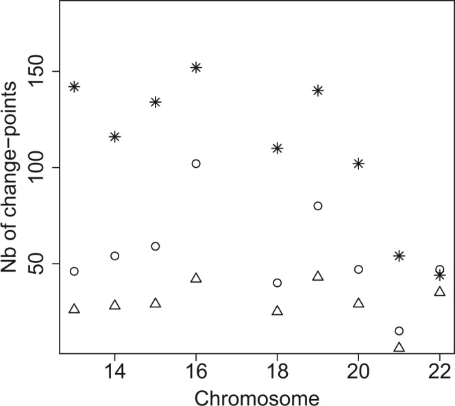
Number of change-points for the Chromosomes 13–22 found by the Bing Ren approach (‘*’), by HiCseg with Model (5) (P) (‘ˆ’) and (5) (B) (‘△’)

Fig. 5.

Left: Log-likelihood (up to some constants) as a function of K for the analysis of Chromosome 15 using Model (5) (P). The dotted vertical lines is the number of blocks chosen by the Dixon et al. (2012) approach, and the solid one correspond to the one of our approach. Right: The same for Chromosome 19 using Model (5) (B)

We also compared both methodologies by computing the two parts of the Hausdorff distance defined in (12) and (13) for Chromosomes 13–22. More precisely, Figure 6 displays the boxplots of the d₁ and d₂ parts of the Hausdorff distance without taking the supremum. We can observe from this figure that some differences exist between the segmentations produced by the two approaches, but that the boundaries of the blocks are close.

Fig. 6.

Boxplots for the infimum parts of the Hausdorff distances d₁ (left part) and d₂ (right part) between the change-points found by Dixon et al. (2012) and our approach for Chromosomes 13–22 for Model (5) (P) [(a) and (b)] and for Model (5) (B) [(c) and (d)]

To further illustrate the differences that exist between both approaches, we display in Figures 7 and 8 the segmentations provided by both approaches in the case of Chromosomes 17 and 19, respectively. In the case of Chromosome 17, we can only provide the segmentation obtained with Model (5) (P) because the overdispersion parameter is infinite (the mean and the variance outside the diagonal blocks are of the same order). In the other case where Models (5) (P) and (B) can be applied, we used the following test procedure for overdispersion under the Poisson model to decide between both segmentations. 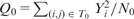Considering the data lying in T₀ as defined in (8), we first estimate the mean within this region by 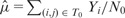where N₀ stands for the number of data points within T₀. We then consider the test statistic . Reminding that, if Y has a Poisson distribution with mean μ, we have and 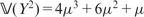, it follows that

under the hypothesis that all observations from T₀ arise from the same Poisson distribution.

Following this rule, we chose Model (5) (B) only for Chromosomes 1 and 2. We can see from this figure that with the naked eye, the diagonal blocks found with our strategy present a lot of similarities with those found by Dixon et al. (2012). We did not report the segmentations that we obtained for the Chromosomes 1–22, but they are available from the Web page of the corresponding author http://www.agroparistech.fr/mmip/maths/essaimia/_media/equipes:membres:page:supplementary_eccb.pdf.

4 CONCLUSION

4.1 HiCseg R package

In this article, we propose a new method for detecting cis-interacting regions in Hi-C data and compare it with a methodology proposed by Dixon et al. (2012). Our approach described in Section 2 is implemented in the R package HiCseg, which is available from the Web page of the corresponding author http://www.agroparistech.fr/mmip/maths/essaimia/_media/equipes:membres:page:hicseg_1.1.tar.gz and from the Comprehensive R Archive Network. In the course of this study, we have shown that HiCseg is an efficient technique for achieving such a segmentation based on a maximum likelihood approach. More precisely, HiCseg package has two main features, which make it attractive. Firstly, it gives access to the exact solution of the maximum likelihood approach. Secondly, as we can see from Figure 9 and Table 1, which give the computational times on synthetic data following Models (5) (G), (P) or (B), HiCseg is computationally efficient, which makes its use possible on real data coming from Hi-C experiments. Note that the computational times of Figure 9 were obtained with a computer having the following configuration: RAM 3.8 GB, CPU 1.6 GHz and those of Table 1 with a computer having the following configuration: RAM 33 GB, CPU 8 × 2.3 GHz.

Fig. 9.

Computational times for Model (5) (G) (‘ˆ’), (P) (‘▲’) and (B) (‘•’)

Table 1.

Computational times (in seconds) for Model (5) (G), (P) and (B)

n	1000	2000	3000	4000	5000	6000	7000
(G)	1.96	17.01	60.56	143.68	280.53	513.87	834.01
(P)	1.92	16.47	57.22	134.91	264.15	453.99	755.21
(B)	1.95	16.60	58.07	135.52	264.62	457.15	783.05

4.2 Open questions

Our methodology could be extended, both to improve the algorithmic efficiency of our method and the modeling of the data.

On the one hand, all available approaches work with data binned at the resolution of several kb. However, the original data are collected at the nucleotide resolution. One of the main challenges would be to alleviate the computational burden of the algorithm to fully take advantage of the Hi-C technology high resolution. Recent advances in segmentation algorithms for 1D data, such as those proposed by Killick et al. (2012) or Rigaill (2010), seem promising for dealing with this issue.

On the other hand, the modeling could be improved in two directions. First, as observed by Phillips-Cremins et al. (2013), Hi-C interaction matrices display a hierarchical structure corresponding to regions interacting at different scales. The proposed segmentation model does not account for such a structure but could be improved in such a direction. Second, a more refined modeling of the dispersion could be considered. While assuming a common dispersion parameter for non-diagonal blocks is sensible because the signal is very low (and therefore, there is little room for large changes in dispersion), the strategy that we propose could incorporate non-homogeneous dispersion parameters for the diagonal blocks. This could be achieved, for instance, by estimating a dispersion parameter per diagonal block. Note that these two extensions could be implemented in the same efficient algorithmic framework as the one proposed in the article. These extensions will be the subject of a future work.

REFERENCES

- Bellman R. On the approximation of curves by line segments using dynamic programming. Commun. ACM. 1961;4:284. [Google Scholar]
- Boysen L, et al. Consistencies and rates of convergence of jump penalized least squares estimators. Ann. Stats. 2009;37:157–183. [Google Scholar]
- Darbon J, Sigelle M. Image restoration with discrete constrained total variation—part I: Fast and exact optimization. J. Math. Imaging Vision. 2006a;26:261–276. [Google Scholar]
- Darbon J, Sigelle M. Image restoration with discrete constrained total variation—part II: Levelable functions, convex priors and non-convex case. J. Math. Imaging Vision. 2006b;26:277–291. [Google Scholar]
- Dixon JR, et al. Topological domains in mammalian genomes identified by analysis of chromatin interactions. Nature. 2012;485:376–380. doi: 10.1038/nature11082. [DOI] [PMC free article] [PubMed] [Google Scholar]
- Fraser J, et al. Chromatin conformation signatures of cellular differentiation. Genome Biol. 2009;10:R37. doi: 10.1186/gb-2009-10-4-r37. [DOI] [PMC free article] [PubMed] [Google Scholar]
- Harchaoui Z, Lévy-Leduc C. Multiple change-point estimation with a total variation penalty. J. Am. Statis. Assoc. 2010;105:1480–1493. [Google Scholar]
- Hochbaum DS. An efficient algorithm for image segmentation, markov random fields and related problems. J. ACM. 2001;48:686–701. [Google Scholar]
- Killick R, et al. Optimal detection of changepoints with a linear computational cost. J. Am. Statis. Assoc. 2012;107:1590–1598. [Google Scholar]
- Lavielle M. Using penalized contrasts for the change-point problem. Signal Proc. 2005;85:1501–1510. [Google Scholar]
- Lieberman-Aiden E, et al. Comprehensive mapping of long-range interactions reveals folding principles of the human genome. Science. 2009;326:289–293. doi: 10.1126/science.1181369. [DOI] [PMC free article] [PubMed] [Google Scholar]
- Nora EP, et al. Spatial partitioning of the regulatory landscape of the x-inactivation centre. Nature. 2012;485:381–385. doi: 10.1038/nature11049. [DOI] [PMC free article] [PubMed] [Google Scholar]
- Phillips-Cremins JE, et al. Architectural protein subclasses shape 3D organization of genomes during lineage commitment. Cell. 2013;153:1281–1295. doi: 10.1016/j.cell.2013.04.053. [DOI] [PMC free article] [PubMed] [Google Scholar]
- Picard F, et al. A statistical approach for array CGH data analysis. BMC Bioinformatics. 2005;6:27. doi: 10.1186/1471-2105-6-27. www.biomedcentral.com/1471-2105/6/27. [DOI] [PMC free article] [PubMed] [Google Scholar]
- Rigaill G. Pruned dynamic programming for optimal multiple change-point detection. ArXiv. 2010 1004.0887. [Google Scholar]