

Abstract
Motivation: Imaging genetics is an emerging field that studies the influence of genetic variation on brain structure and function. The major task is to examine the association between genetic markers such as single-nucleotide polymorphisms (SNPs) and quantitative traits (QTs) extracted from neuroimaging data. The complexity of these datasets has presented critical bioinformatics challenges that require new enabling tools. Sparse canonical correlation analysis (SCCA) is a bi-multivariate technique used in imaging genetics to identify complex multi-SNP–multi-QT associations. However, most of the existing SCCA algorithms are designed using the soft thresholding method, which assumes that the input features are independent from one another. This assumption clearly does not hold for the imaging genetic data. In this article, we propose a new knowledge-guided SCCA algorithm (KG-SCCA) to overcome this limitation as well as improve learning results by incorporating valuable prior knowledge.
Results: The proposed KG-SCCA method is able to model two types of prior knowledge: one as a group structure (e.g. linkage disequilibrium blocks among SNPs) and the other as a network structure (e.g. gene co-expression network among brain regions). The new model incorporates these prior structures by introducing new regularization terms to encourage weight similarity between grouped or connected features. A new algorithm is designed to solve the KG-SCCA model without imposing the independence constraint on the input features. We demonstrate the effectiveness of our algorithm with both synthetic and real data. For real data, using an Alzheimer’s disease (AD) cohort, we examine the imaging genetic associations between all SNPs in the APOE gene (i.e. top AD gene) and amyloid deposition measures among cortical regions (i.e. a major AD hallmark). In comparison with a widely used SCCA implementation, our KG-SCCA algorithm produces not only improved cross-validation performances but also biologically meaningful results.
Availability: Software is freely available on request.
Contact: shenli@iu.edu
1 INTRODUCTION
Brain imaging genetics is an emerging field that studies the influence of genetic variation on brain structure and function. Its major task is to examine the association between genetic markers such as single-nucleotide polymorphisms (SNPs) and quantitative traits (QTs) extracted from multimodal neuroimaging data (e.g. anatomical, functional and molecular imaging scans). Given the well-known importance of gene and imaging phenotype in brain function, bridging these two factors and exploring their connections would lead to a better mechanistic understanding of normal or disordered brain functions. The complexity of these data, however, has presented critical bioinformatics challenges requiring new enabling tools. Early studies in imaging genetics typically focused on pairwise univariate analysis (Shen et al., 2010). Many recent studies turned to regression analysis for exploring the joint effect of multiple SNPs on single or few QTs (Hibar et al., 2011) and bi-multivariate analyses for revealing complex multi-SNPs–multi-QTs associations (Chi et al., 2013; Lin et al., 2014; Vounou et al., 2010; Wan et al., 2011).
Canonical correlation analysis (CCA), a bi-multivariate method, has been applied to imaging genetics applications. It aims to find the best linear transformation for imaging and genetics features so that the highest correlation between imaging and genetic components can be achieved. Based on the assumption that a real imaging genetic signal typically involves a small number of SNPs and QTs, sparse canonical correlation analysis (SCCA) has also been applied in several imaging genetic studies by imposing the Lasso regularization term to yield sparse results (Chi et al., 2013; Lin et al., 2014; Wan et al., 2011). However, most existing SCCA algorithms are designed using the soft thresholding technique, which assumes that the input features are independent from one another (Tibshirani, 1996). This assumption clearly does not hold for the imaging genetic data [e.g. the existence of the structural and functional networks in the brain and the linkage disequilibrium (LD) blocks in the genome]. Directly ignoring the covariance structure in the data will inevitably limit the capability of yielding optimal results.
In this article, we propose a new knowledge-guided SCCA algorithm (KG-SCCA) to overcome this limitation as well as to aim for improving learning results by incorporating valuable prior knowledge. The proposed KG-SCCA method is able to model two types of prior knowledge: one as a group structure (e.g. LD blocks among SNPs) and the other as a network structure (e.g. gene co-expression network among brain regions). The new model incorporates these prior structures by introducing new regularization terms to encourage similarity between grouped or connected features. A new algorithm is designed to solve the KG-SCCA model without imposing the independence constraint on the input features. We demonstrate the effectiveness of our algorithm with both synthetic and real data. For real data, using an Alzheimer’s disease (AD) cohort, we examine the imaging genetic associations between all SNPs in the APOE gene (i.e. top AD gene) and amyloid deposition measures among cortical regions (i.e. a major AD hallmark). In comparison with a widely used SCCA implementation in the PMA software package (http://cran.r-project.org/web/packages/PMA/) (Witten et al., 2009), our KG-SCCA algorithm produces improved cross-validation performances as well as biologically meaningful results.
2 MATERIALS AND DATA SOURCES
To demonstrate the proposed KG-SCCA algorithm, we apply it to an amyloid imaging genetic analysis in the study of AD. Deposition of amyloid-β in the cerebral cortex is a major hallmark in AD pathogenesis. Our prior studies (Ramanan et al., 2014; Swaminathan et al., 2012) performed univariate genetic association analyses of amyloid measures in a few candidate cortical regions of interest (ROIs), and identified several promising hits including rs429358 in APOE, rs509208 in BCHE and rs7551288 in DHCR24. In this work, using the proposed KG-SCCA algorithm, we perform a bi-multivariate analysis to examine the association between all the available SNPs (58 in total) in the APOE gene (i.e. the top genetic risk factor for late onset AD) and 78 ROIs across the entire cortex. We use two types of prior knowledge in this analysis: (i) a group structure is imposed to the SNP data using the LD block information (Fig. 4), and (ii) a network structure is imposed to the amyloid imaging data by computing an amyloid pathway-based gene co-expression network in the brain using Allen Human Brain Atlas (AHBA; Zeng et al., 2012). Below, we first describe our amyloid imaging and genotyping data, and then discuss our method for creating the amyloid pathway-based gene co-expression network in the brain.
Fig. 4.

Five-fold trained weights of u (top panel) and v (bottom panel). KG-SCCA results and PMA results are shown for each panel. For each of KG-SCCA and PMA imaging results (i.e. the bottom panel), the top and bottom rows correspond to left and right hemispheres, respectively
2.1 Imaging and genotyping data
The proposed algorithm, KG-SCCA, was empirically evaluated using the amyloid imaging and genotyping data obtained from the Alzheimer’s Disease Neuroimaging Initiative (ADNI) database (adni.loni.usc.edu). One goal of ADNI has been to test whether serial magnetic resonance imaging (MRI), positron emission tomography (PET), other biological markers and clinical and neuropsychological assessment can be combined to measure the progression of mild cognitive impairment (MCI) and early AD. For up-to-date information, see www.adni-info.org. Preprocessed [18F]Florbetapir PET scans (i.e. amyloid imaging data) were downloaded from LONI (adni.loni.usc.edu). Before downloading, images were averaged, aligned to a standard space, resampled to a standard image and voxel size, smoothed to a uniform resolution and normalized to a cerebellar gray matter reference region resulting in standardized uptake value ratio images as previously described (Jagust et al., 2010). After downloading, the images were aligned to each participant’s same visit MRI scan and normalized to the Montreal Neurological Institute (MNI) space as 2 × 2 × 2 mm voxels using parameters from the MRI segmentation. ROI level amyloid measurements were further extracted based on the MarsBaR AAL atlas. Genotype data of both ADNI-1 and ADNI-2/GO phases were also obtained from LONI (adni.loni.usc.edu). All the APOE SNPs were extracted based on the quality controlled and imputed data combining two phases together. Only SNPs available in Illumina 610Quad and/or OmniExpress arrays were included in the analysis. As a result, we had 58 SNPs located within 10 LD blocks (Fig. 4) computed using HaploView (Barrett, 2009). A total of 568 non-Hispanic Caucasian participants with both complete amyloid measurements and APOE SNPs were studied, including 28 AD, 343 MCI and 196 healthy control (HC) subjects (Table 1). Using the regression weights derived from the HC participants, amyloid and SNP measures were preadjusted for removing the effects of the baseline age, gender, education and handedness.
Table 1.
Participant characteristics
| Subjects | AD | MCI | HC |
|---|---|---|---|
| Number | 28 | 343 | 196 |
| Gender (M/F) | 18/10 | 203/140 | 102/94 |
| Handedness (R/L) | 23/5 | 309/34 | 178/18 |
| Age (mean ± std) | 75.23 ± 10.66 | 71.92 ± 7.47 | 74.77 ± 5.39 |
| Education (mean ± std) | 15.61 ± 2.74 | 15.99 ± 2.75 | 16.46 ± 2.65 |
2.2 Amyloid pathway-based gene co-expression network in the brain
Because we examine cortical amyloid deposition in relation to genetic variation, we hypothesize that amyloid pathway-based gene co-expression profiles among cortical ROIs may provide valuable information in search for APOE-related amyloid distribution pattern in the cortex. Thus, we used the brain transcriptome data from the AHBA (Zeng et al., 2012), coupled with 15 candidate genes from amyloid pathways studied in (Swaminathan et al., 2012), to create such a brain network.
Gene expression profiles across the whole human brain were downloaded from Allen Institute for Brain Science. One of their goals is to advance the research and knowledge about neurobiological conditions, with extensive mapping of whole-genome gene expression throughout the brain. Among various organisms, AHBA is one of the projects seeking to combine the genomics with the neuroanatomy to better understand the connection between genes and brain functioning. Gene expression profiles in eight health human brains have been released, including two full brains and six right hemispheres. Details can be found in www.brain-map.org.
Brain-wide expression data of all 15 amyloid-related candidate genes, reported in (Swaminathan et al., 2012), were extracted from AHBA to construct the brain network. Because an early report indicated that individuals share as much as 95% gene expression profile (Zeng et al., 2012), in this study, we only included two full brains (H0351-2201 and H0351-2002) to construct the co-expression network. First all the brain samples (∼900) in AHBA were mapped to MarSBAR AAL atlas, which included 116 brain ROIs. According to Ramanan et al. (2014), cortical ROIs are typically believed to hold the amyloid signals, whereas other ROIs hold similar amyloid measures across individuals. Thus, 39 pairs of bilateral cortical ROIs (78 in total), from frontal lobe, cingulate, parietal lobe, temporal lobe, occipital lobe, insula and sensory–motor cortex, were included in our analysis. Correlation among ∼900 brain locations was first calculated based on the gene expression profile of 15 amyloid candidate genes. Due to many-to-one mapping from the brain locations to AAL ROIs, for each ROI, there are more than one connections, represented by correlations between two brain locations. Therefore, we calculated ROI-level correlations of two individuals in five ways: minimum, maximum, mean, standard deviation and median. In addition, the ROI correlation structure based on the combination of both individuals was also generated in the same way for comparison (Fig. 1). Clearly, for all five statistics, the pattern remains highly consistent across individuals and their combination. For simplicity, in the subsequent analysis, we adopt the brain connectivity matrix generated from the combination sample using the median statistics (i.e. the panel in the lower right corner of Fig. 1). Figure 2 shows a network visualization of this matrix, where edges correspond to matrix entries with values or .
Fig. 1.
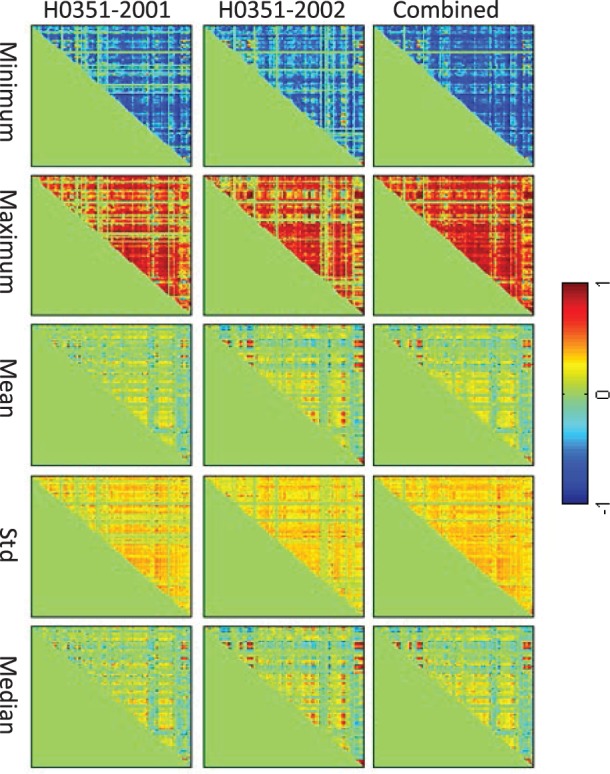
Amyloid pathway-based gene co-expression networks among 78 AAL cortical ROIs constructed from AHBA using different statistics (see different rows) for two individuals and their combination
Fig. 2.
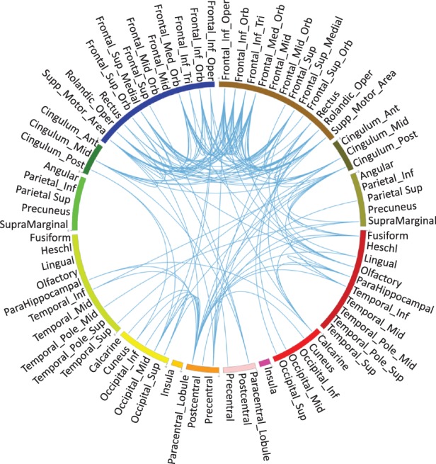
Network visualization by thresholding the connectivity matrix shown in the lower right corner of Figure 1, where edges correspond to matrix entries with values or . The circle is symmetric (left measures on left and right measures on right), from top to bottom are frontal lobe, cingulate, parietal lobe, temporal lobe, occipital lobe, insula and sensory–motor cortex
3 METHODS
Now we present our KG-SCCA algorithm. We denote vectors as boldface lowercase letters and matrices as boldface uppercase ones. For a given matrix , we denote its i-th row and j-th column as and , respectively. Let be the genotype data (SNP) and be the imaging QT data, where n is the number of participants, p and q are the numbers of SNPs and QTs, respectively.
CCA seeks linear transformations of variables X and Y to achieve the maximal correlation between Xu and Yv, which can be formulated as:
| (1) |
where u and v are canonical loadings or weights, reflecting the significance of each feature in the identified canonical correlation.
Similar to many machine learning algorithms, overfitting could arise in CCA when the features outnumber the participants. In addition, the CCA outcome could spread non-trivial effects across all the features rather than only a few significant ones, making the results difficult to interpret. To address these issues, SCCA was proposed in (Witten et al., 2009) by introducing penalty terms, and , to regularize the weights, as shown in Equation (2).
| (2) |
Here the objective function is bilinear in u and v: when u is fixed, it is linear in v and vice versa. But due to the L2 equality, with u or v fixed, the constraints are not convex. This can be solved by reformulating the L2 equality into inequality as and . For easy computation, Equation (2) is commonly rewritten in its Lagrangian form.
| (3) |
Witten et al. (2009) and Witten and Tibshirani (2009) explored two penalty forms, L1 penalty and the chain structured fused Lasso penalty. L1 penalty imposes sparsity on both u and v and assumes that each canonical correlation involves only a few features from X and Y. The fused Lasso penalty promotes the smoothness of weight vectors and encourages neighboring features to be selected together. To incorporate other structures, group- and network-guided penalties were introduced (Chen and Liu, 2012; Chen et al., 2013). As mentioned earlier, most of these methods were designed using the soft thresholding technique, which was first proposed to solve Lasso problem when the features were independent from each other (Tibshirani, 1996). This condition does not hold in imaging genetics data. Thus, direct application of those methods into imaging genetics studies limits the capability of yielding optimal solutions. Below, we first present our KG-SCCA model and then present an effective KG-SCCA algorithm without using the soft thresholding strategy.
Brain has been studied as a complicated network. The SNP data have structures like LD blocks. Given these prior knowledge, we propose the following KG-SCCA model by introducing two penalty terms for genetic loadings u and imaging loading v, respectively.
| (4) |
In penalty , SNPs are partitioned into K1 groups , such that , and is the number of SNPs in . While the group term helps select all the SNPs in relevant LD blocks, L1 penalty manages to suppress those non-signals within selected LD blocks. The penalty is essentially the group Lasso penalty applied to the CCA framework.
Penalty applies the network-guided constraint to encourage the joint selection of ‘connected’ features (i.e. their connectivity matrix entry having a high weight) as well as uses L1 to impose global sparsity. E is the set of all possible imaging QT pairs and is the total number of QT pairs. is defined as follows. The row of C is indexed by all pairs and . provide the fusion effect that promotes similarity between vi and vj of related features. In this article, we use . With we can have positively related features being pulled together and on the other hand the negatively related features being fused with opposite direction. Thus, for strongly connected features with a large fusion effect, they tend to be jointly selected or jointly not selected.
In this work, as mentioned earlier, we formed the group structure for the SNP data by partitioning them using LD blocks generated by HaploView (Barrett, 2009). We formed the network structure for the amyloid imaging data by constructing amyloid pathway-based gene co-expression network using AHBA. Because the model could be easily extended to estimate multiple canonical variables, we only focus on creating the first pair of canonical variables in this article.
Algorithm 1 Knowledge-guided SCCA (KG-SCCA).
Require:
, group and network structures
Ensure:
Canonical vectors u and v.
1: t = 1, Initialize ;
2: while not converge do
3: Calculate
4: Calculate the block diagonal matrix and ;
5: ;
6: Scale so that ;
7: Calculate ;
8: Calculate the block diagonal matrix ;
9: ;
10: Scale so that ;
11: .
12: end while
We now present our algorithm to solve this model without using soft thresholding approach. By fixing u and v, respectively, we will have two convex problems shown in Equation (5).
| (5) |
Let and , the above problems can be reformulated to Equation (6):
| (6) |
Here, while u can be solved by the G-SMuRFS method proposed in (Wang et al., 2012), optimization of v can be achieved by the network-guided regression method proposed in (Yan et al., 2013). In both solutions, a smooth approximation has been estimated for group and L1 terms by including an extremely small value. The solution for u and v in each iteration step is as follows:
| (7) |
where is a block diagonal matrix with the k-th diagonal block as ; is an identity matrix with size of mk; mk is the total feature number in group k; is a diagonal matrix with the i-th diagonal element as ; = is a matrix in which each row integrates all the neighboring relationships (e.g. for the i-th row, it is the sum of all the rows in α whose i-th element is not zero); and is a diagonal matrix with the i-th diagonal element as . Algorithm 1 summarizes the KG-SCCA optimization procedure. Further details on how to solve for two objectives in Equation (6) are available in (Wang et al., 2012) and (Yan et al., 2013), respectively.
In Algorithm 1, six parameters need to be tuned to control the global sparsity as well as structured group or network constraints. Chen and Liu (2012) studied a similar problem using a different method, and found that their results were insensitive to settings. Following their observation, we set to 1 for simplicity. Nested cross-validation can be used for parameter selection but will be extremely time-consuming for the remaining four parameters. Thus, we followed the strategy proposed in (Lin et al., 2014): parameters controlling structural constraints were first tuned without considering sparsity constraints. Then based on the obtained optimal , another nested cross-validation was performed to acquire the optimal .
4 EXPERIMENTAL RESULTS AND DISCUSSIONS
We performed comparative studies between the proposed KG-SCCA algorithm and a widely used SCCA implementation in the PMA package (http://cran.r-project.org/web/packages/PMA/) (Witten et al., 2009). For PMA experiments, the SCCA parameters were automatically tuned using a permutation scheme provided in PMA. Below we report our empirical results using both synthetic data and real imaging genetics data.
4.1 Results on simulation data
Because it was not straightforward to manually construct a dataset with a network structure, we simulated group structures for both datasets and then converted them into network structures for one dataset by connecting all the pairs within each group. Synthetic data () with diagonal block structure was generated with the following procedure: (i) Random positive definite covariance matrix M with non-overlapping group structure was created, where correlations range from 0.6 to 1 within group and are set to 0 between groups. (ii) Dataset X with covariance structure M was calculated through Cholesky decomposition. (iii) Repeat Steps 1 and 2 to generate another dataset Y. (iv) With assigned canonical loadings of X, we calculated the first component Xu. (v) Given a desired correlation between components, we calculated the second component Yv. (vi) For simplicity, in this article, only one group in Y was assigned to have signals. Therefore, based on predefined canonical loadings of Y and component Yv, final obtained group signals, added with some white noises (Signal to Noise Ratio (SNR) = 0.5), will replace the data in original dataset Y. By repeating this procedure we generated seven datasets with correlation levels from 0.6 to 1. The canonical loadings and group structure remained the same across all the datasets.
KG-SCCA and PMA have been both tested on all seven datasets. All the regularization parameters were optimally tuned using a grid search from to 102 through nested 5-fold cross-validation, as mentioned before. The true and estimated canonical loadings for both X and Y were shown in Figure 3. Owing to the difference in normalization and optimization procedure, the weights yielded by KG-SCCA and PMA showed different scales. Yet, the overall profile of the estimated u and v values from KG-SCCA kept consistent with the ground truth across the entire range of tested correlation strengths (from 0.6 to 1.0), whereas PMA was only capable of identifying an incomplete portion of all the signals. Furthermore, we also examined the correlation in the test set computed using the learned models from the training data for both methods. The left part of Table 2 demonstrated that KG-SCCA outperformed PMA consistently and significantly, and it could accurately reveal the embedded true correlation even in the test data. The right part of Table 2 demonstrated the sensitivity and specificity performance using area under ROC (AUC), where KG-SCCA also significantly outperformed PMA no matter whether the correlation was weak or strong in u. Because v is relatively simple structured, both KG-SCCA and PMA can restore the signals without any loss. From the above results, it is also observed that KG-SCCA could identify the correlations and signal locations not only more accurately but also more stably.
Fig. 3.
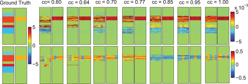
Five-fold trained weights of u and v. Ground truth of u and v are shown in the most left two panels. KG-SCCA results (top row) and PMA results (bottom row) are shown in the remaining panels, corresponding to true correlation coefficients (CCs) ranging from 0.6 to 1.0. For each panel pair, the five estimated u values are shown on the left panel, and the five estimated v values are shown on the right panel
Table 2.
Five-fold cross-validation performance on synthetic data: mean ± std is shown for estimated correlation coefficients and AUC of the test data using the trained model
| True | Correlation coefficients (CC) |
AUC |
||||||
|---|---|---|---|---|---|---|---|---|
| CC | KG-SCCA | PMA | P | KG-SCCA:u | PMA:u | P | KG-SCCA:v | PMA:v |
| 0.60 | 0.56 ± 0.12 | 0.31 ± 0.14 | 2.19E-03 | 0.83 ± 0.08 | 0.64 ± 0.02 | 3.36E-03 | 1.0 ± 0.00 | 1.0 ± 0.00 |
| 0.64 | 0.56 ± 0.1 | 0.51 ± 0.12 | 2.32E-02 | 0.96 ± 0.04 | 0.65 ± 0.01 | 2.20E-05 | 1.0 ± 0.00 | 1.0 ± 0.00 |
| 0.70 | 0.64 ± 0.1 | 0.53 ± 0.1 | 1.27E-05 | 0.99 ± 0.01 | 0.62 ± 0. | 6.21E-08 | 1.0 ± 0.00 | 1.0 ± 0.00 |
| 0.77 | 0.7 ± 0.14 | 0.6 ± 0.14 | 6.62E-03 | 0.99 ± 0.01 | 0.62 ± 0. | 9.67E-09 | 1.0 ± 0.00 | 1.0 ± 0.00 |
| 0.85 | 0.76 ± 0.08 | 0.65 ± 0.1 | 1.02E-04 | 0.98 ± 0.03 | 0.63 ± 0.01 | 4.57E-06 | 1.0 ± 0.00 | 1.0 ± 0.00 |
| 0.95 | 0.87 ± 0.04 | 0.67 ± 0.09 | 1.19E-03 | 1.00 ± 0.00 | 0.63 ± 0.01 | 1.39E-08 | 1.0 ± 0.00 | 1.0 ± 0.00 |
| 1.00 | 0.92 ± 0.04 | 0.71 ± 0.06 | 2.46E-04 | 1.00 ± 0.00 | 0.64 ± 0.01 | 4.02E-08 | 1.0 ± 0.00 | 1.0 ± 0.00 |
Note. P-value of paired t-test between KG-SCCA and PMA results are also shown.
4.2 Results on real imaging genetic data
Both KG-SCCA and PMA have been performed on real amyloid imaging and APOE genetics data. Similar to previous analysis, 5-fold nested cross-validation was applied to optimally tune the parameters. Five experiments were performed with five different partitions to eliminate the bias. For each single experiment, the same partition was used for both KG-SCCA and PMA. Table 3 shows both the training and test performances of KG-SCCA and PMA in all five folds of five experiments. Both methods demonstrated stable results across five trials. KG-SCCA was observed to outperform the PMA in every single experiment on both training and test performance. Paired t-test was performed to compare the performance across five experiments, and KG-SCCA outperformed PMA significantly in both training (P = 3.08E-6) and test cases (P = 8.07E-5). We also tested two simplified KG-SCCA models: one with only the penalty term for the LD structure and the other with only the penalty term for the network structure. Interestingly, both performed similarly to the original KG-SCCA, and significantly outperformed PMA.
Table 3.
Five-fold cross validation results on real data: the models learned from the training data were used to estimate the correlation coefficients between canonical components for both training and testing sets
| Method |
Train |
Test |
|||||||||||
|---|---|---|---|---|---|---|---|---|---|---|---|---|---|
| f1 | f2 | f3 | f4 | f5 | Mean | f1 | f2 | f3 | f4 | f5 | Mean | ||
| KG-SCCA | exp1 | 0.471 | 0.448 | 0.475 | 0.451 | 0.46 | 0.461 | 0.431 | 0.515 | 0.401 | 0.417 | 0.459 | 0.445 |
| exp2 | 0.476 | 0.453 | 0.454 | 0.476 | 0.461 | 0.464 | 0.402 | 0.505 | 0.503 | 0.401 | 0.458 | 0.454 | |
| exp3 | 0.476 | 0.474 | 0.474 | 0.468 | 0.402 | 0.459 | 0.408 | 0.393 | 0.413 | 0.435 | 0.565 | 0.443 | |
| exp4 | 0.468 | 0.466 | 0.459 | 0.46 | 0.466 | 0.464 | 0.441 | 0.409 | 0.47 | 0.476 | 0.445 | 0.448 | |
| exp5 | 0.49 | 0.502 | 0.434 | 0.449 | 0.447 | 0.464 | 0.35 | 0.297 | 0.584 | 0.527 | 0.528 | 0.457 | |
| PMA | exp1 | 0.439 | 0.418 | 0.438 | 0.438 | 0.426 | 0.432 | 0.368 | 0.45 | 0.398 | 0.379 | 0.439 | 0.407 |
| exp2 | 0.444 | 0.416 | 0.425 | 0.436 | 0.432 | 0.431 | 0.354 | 0.463 | 0.449 | 0.399 | 0.416 | 0.416 | |
| exp3 | 0.442 | 0.445 | 0.439 | 0.427 | 0.398 | 0.43 | 0.382 | 0.341 | 0.382 | 0.432 | 0.544 | 0.416 | |
| exp4 | 0.434 | 0.44 | 0.425 | 0.427 | 0.431 | 0.432 | 0.414 | 0.363 | 0.445 | 0.438 | 0.415 | 0.415 | |
| exp5 | 0.459 | 0.462 | 0.406 | 0.416 | 0.411 | 0.431 | 0.288 | 0.287 | 0.517 | 0.486 | 0.501 | 0.416 | |
| P-value | 3.08E-6 | P-value | 8.07E-5 | ||||||||||
Note. P-values of paired t-tests were obtained for comparing KG-SCCA and PMA results.
Figure 4 demonstrates the canonical loadings trained from 5-fold cross-validation in one experiment, suggesting relevant genetic (top panel) and imaging (bottom panel) markers. Although LD block constraints were imposed on relevant SNP markers, L1 penalty managed to exclude irrelevant signals. Only APOE e4 SNP (rs429358) was identified to be associated with amyloid accumulations in the brain. PMA also achieved a similar pattern as KG-SCCA, but including a few additional SNPs from multiple LD blocks. The bottom panel of Figure 4 shows the canonical loading for the imaging data. Both methods identified similar imaging patterns, which are in accordance with prior findings (Ramanan et al., 2014). Figure 5 shows a brain map of canonical loadings generated by KG-SCCA.
Fig. 5.
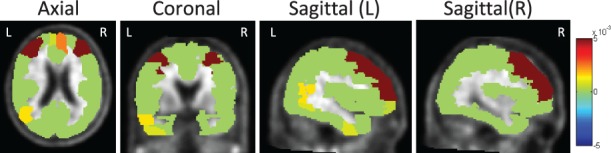
Mapping canonical loading generated by KG-SCCA onto the brain
5 CONCLUSIONS
We have performed a brain imaging genetics study to explore the relationship between brain-wide amyloid accumulation and genetic variations in the APOE gene. Because most existing SCCA algorithms are designed using the soft thresholding technique, which assumes independence among data features, direct application of these methods into brain imaging genetics study cannot yield optimal results owing to the correlated imaging and genetic features. We have proposed a novel KG-SCCA algorithm, which not only removes the above independence assumption, but also can model both the group-like and network-like prior knowledge in the data to produce improved learning results. A comparative study has been performed between KG-SCCA and PMA (a widely used SCCA implementation) on both synthetic and real data. The promising empirical results demonstrated that KG-SCCA significantly outperformed PMA in both cases. Furthermore, KG-SCCA could accurately recover the true signals from the synthetic data, as well as yield improved canonical correlation performances and biologically meaningful findings from real data. This study is an initial attempt to remove the feature independence assumption many existing SCCA methods have. The empirical studies designed here are targeted to identify relatively clean and simple multi-SNP–multi-QT correlations. Given only 58 SNPs analyzed here, this work is not a demonstration of a genome-wide analysis. Comparison with other complex SCCA models, building scalable KG-SCCA models, and applications to more complex imaging genetic tasks warrant further investigation.
ACKNOWLEDGEMENTS
Detailed ADNI Acknowledgements information is available in http://adni.loni.usc.edu/wp-content/uploads/how_to_apply/ADNI_Manuscript_Citations.pdf. Data used in preparation of this article were obtained from the Alzheimer’s Disease Neuroimaging Initiative (ADNI) database (adni.loni.usc.edu). As such, the investigators within the ADNI contributed to the design and implementation of ADNI and/or provided data but did not participate in analysis or writing of this report. A complete listing of ADNI investigators can be found at: http://adni.loni.usc.edu/wp-content/uploads/how_to_apply/ADNI_Acknowledgement_List.pdf.
Funding: This work was supported by the National Institutes of Health [R01 LM011360 to L.S. and A.S., U01 AG024904 to M.W. and A.S., RC2 AG036535 to M.W. and A.S., R01 AG19771 to A.S., P30 AG10133 to A.S.] and the National Science Foundation [IIS-1117335 to L.S.] at IU; by the National Science Foundation [IIS-1117965 to H.H., IIS-1302675 to H.H., IIS-1344152 to H.H., DBI-1356628 to H.H.] at UTA; and by the National Institutes of Health [R01 LM011360 to J.M., R01 LM009012 to J.M., R01 LM010098 to J.M.] at Dartmouth.
Conflict of interest: none declared.
REFERENCES
- Barrett JC. Haploview: visualization and analysis of SNP genotype data. Cold Spring Harb. Protoc. 2009;2009:pdb ip71. doi: 10.1101/pdb.ip71. [DOI] [PubMed] [Google Scholar]
- Chen J, et al. Structure-constrained sparse canonical correlation analysis with an application to microbiome data analysis. Biostatistics. 2013;14:244–258. doi: 10.1093/biostatistics/kxs038. [DOI] [PMC free article] [PubMed] [Google Scholar]
- Chen X, Liu H. An efficient optimization algorithm for structured sparse CCA, with applications to eQTL mapping. Stat. Biosci. 2012;4:3–26. [Google Scholar]
- Chi E, et al. Biomedical Imaging (ISBI), 2013 IEEE 10th Int Sym on. San Francisco, USA: 2013. Imaging genetics via sparse canonical correlation analysis; pp. 740–743. [DOI] [PMC free article] [PubMed] [Google Scholar]
- Hibar DP, et al. Multilocus genetic analysis of brain images. Front. Genet. 2011;2:73. doi: 10.3389/fgene.2011.00073. [DOI] [PMC free article] [PubMed] [Google Scholar]
- Jagust WJ, et al. The Alzheimer’s Disease Neuroimaging Initiative positron emission tomography core. Alzheimers Dement. 2010;6:221–229. doi: 10.1016/j.jalz.2010.03.003. [DOI] [PMC free article] [PubMed] [Google Scholar]
- Lin D, et al. Correspondence between fMRI and SNP data by group sparse canonical correlation analysis. Med. Image Anal. 2014;18:891–902. doi: 10.1016/j.media.2013.10.010. [DOI] [PMC free article] [PubMed] [Google Scholar]
- Ramanan VK, et al. APOE and BCHE as modulators of cerebral amyloid deposition: a florbetapir PET genome-wide association study. Mol. Psychiatry. 2014;19:351–357. doi: 10.1038/mp.2013.19. [DOI] [PMC free article] [PubMed] [Google Scholar]
- Shen L, et al. Whole genome association study of brain-wide imaging phenotypes for identifying quantitative trait loci in MCI and AD: A study of the ADNI cohort. Neuroimage. 2010;53:1051–1063. doi: 10.1016/j.neuroimage.2010.01.042. [DOI] [PMC free article] [PubMed] [Google Scholar]
- Swaminathan S, et al. Amyloid pathway-based candidate gene analysis of [(11)C]PiB-PET in the Alzheimer’s Disease Neuroimaging Initiative (ADNI) cohort. Brain Imaging Behav. 2012;6:1–15. doi: 10.1007/s11682-011-9136-1. [DOI] [PMC free article] [PubMed] [Google Scholar]
- Tibshirani R. Regression shrinkage and selection via the lasso. J. R. Stat. Soc. Ser. B. 1996;58:267–288. [Google Scholar]
- Vounou M, et al. Discovering genetic associations with high-dimensional neuroimaging phenotypes: a sparse reduced-rank regression approach. NeuroImage. 2010;53:1147–1159. doi: 10.1016/j.neuroimage.2010.07.002. [DOI] [PMC free article] [PubMed] [Google Scholar]
- Wan J, et al. Hippocampal surface mapping of genetic risk factors in AD via sparse learning models. Med. Image Comput. Comput. Assist. Interv. 2011;14(Pt 2):376–383. doi: 10.1007/978-3-642-23629-7_46. [DOI] [PMC free article] [PubMed] [Google Scholar]
- Wang H, et al. Identifying quantitative trait loci via group-sparse multitask regression and feature selection: an imaging genetics study of the ADNI cohort. Bioinformatics. 2012;28:229–237. doi: 10.1093/bioinformatics/btr649. [DOI] [PMC free article] [PubMed] [Google Scholar]
- Witten DM, Tibshirani RJ. Extensions of sparse canonical correlation analysis with applications to genomic data. Stat. Appl. Genet. Mol. Biol. 2009;8:Article28. doi: 10.2202/1544-6115.1470. [DOI] [PMC free article] [PubMed] [Google Scholar]
- Witten DM, et al. A penalized matrix decomposition, with applications to sparse principal components and canonical correlation analysis. Biostatistics. 2009;10:515–534. doi: 10.1093/biostatistics/kxp008. [DOI] [PMC free article] [PubMed] [Google Scholar]
- Yan J, et al. Multimodal Brain Image Analysis (MBIA), Nagoya, Japan. LNCS 8159. Vol. 8159. Switzerland: Springer International Publishing; 2013. Network-guided sparse learning for predicting cognitive outcomes from MRI measures; pp. 150–158. [DOI] [PMC free article] [PubMed] [Google Scholar]
- Zeng H, et al. Large-scale cellular-resolution gene profiling in human neocortex reveals species-specific molecular signatures. Cell. 2012;149:483–496. doi: 10.1016/j.cell.2012.02.052. [DOI] [PMC free article] [PubMed] [Google Scholar]