AxonQuant: A Microfluidic Chamber Culture-Coupled Algorithm That Allows High-Throughput Quantification of Axonal Damage

Abstract

Published methods for imaging and quantitatively analyzing morphological changes in neuronal axons have serious limitations because of their small sample sizes, and their time-consuming and nonobjective nature. Here we present an improved microfluidic chamber design suitable for fast and high-throughput imaging of neuronal axons. We developed the Axon-Quant algorithm, which is suitable for automatic processing of axonal imaging data. This microfluidic chamber-coupled algorithm allows calculation of an ‘axonal continuity index’ that quantitatively measures axonal health status in a manner independent of neuronal or axonal density. This method allows quantitative analysis of axonal morphology in an automatic and nonbiased manner. Our method will facilitate large-scale high-throughput screening for genes or therapeutic compounds for neurodegenerative diseases involving axonal damage. When combined with imaging technologies utilizing different gene markers, this method will provide new insights into the mechanistic basis for axon degeneration. Our microfluidic chamber culture-coupled AxonQuant algorithm will be widely useful for studying axonal biology and neurodegenerative disorders.

Introduction

Axonal damage is a common and early feature in a large number of neurodegenerative diseases including Alzheimer’s disease, Parkinson’s disease and amyotrophic lateral sclerosis [1–4]. In some cases, it has been demonstrated that axonal impairment not only precedes but also induces neuronal death in a ‘dying back’ mechanism [5]. Although significant effort has been made in studying axonal damage, methods for detecting and quantifying axonal damage in cultured neurons remain limited.

Studying axonal damage quantitatively is challenging because such damage can be triggered by various insults, including injury, toxins, epigenetic changes and genetic defects. In vitro models have been developed for examining axonal morphology by providing controlled culture environment, compound delivery and genetic manipulation, and a shortened experimental time window. In most studies, conventional primary neuronal culture has been used for axon morphological characterization. Different methods have been reported to evaluate axonal damage. The most frequently used method for quantifying axonal morphology is ‘image segmentation’ [6–10], which is employed in commercial software such as MetaMorph and Imaris. This method isolates spot-like discontinuous image components from homogenous regions of an image by automatically detecting the local intensity maxima or threshold segmentation. Recently, a semiautomated ImageJ-based method was reported for quantifying axonal segmentation in microfluidic chamber-cultured neurons [6]. This method relied on manually defining regions of interest (ROI) and ImageJ and therefore only allowed quantification of axons in low-density areas. Another frequently used method for quantifying axonal morphology is ‘filament tracking’ [11, 12], which detects continuity of axons in a semiautomatic manner which also depends on manual definition of the axons to be quantified.

Many of these published methods [6–12] have a number of limitations. First, random selection of imaging fields during the image capture process may introduce subjective errors. Second, because the measurement of axonal abnormality is manual or semimanual in most cases, it is often extremely time-consuming. Third, the lack of objective criteria and an insufficient sample size limit the reliability and sensitivity of analyses. Fourth, in many studies, quantification of axonal morphology was limited to low-density cultures or less-than-mature neurons because extensive overlapping of neuronal processes in high-density culture or mature neurons prevents the definitive identification of individual axons, leading to an inability to quantify axonal morphology under such conditions. These limitations have prevented the use of axonal damage as an effective parameter in high-throughput screening.

Compartmentalized cultures [13–15] for neurons have been improved significantly since the development of the original Campenot chamber [16–19]. The development of micro-fluidic chambers has facilitated compartmentalized neuronal cultures [19]. Axons and cell bodies can be cultured in separate compartments because of their growth properties and morphological features. Such microfluidic chambers also make it possible to reduce the culture scale to a few thousand cells, using a small amount of culture medium in a more precisely defined 3D space. However, published designs of microfluidic chambers for neuronal cultures [15, 20–22] have not been sufficiently developed to incorporate automatic analyses or to allow high-throughput applications. In this study, we redesigned the microfluidic chamber system, using a multiwell format to facilitate the application of an automated image processing and quantification algorithm for studying axonal damage. This combination has produced a standardized platform for analyzing axon integrity in a systematic and high-throughput manner. We provide a high-throughput axon quantification tool kit, Axon-Quant1.0, which includes a neuronal culture using the newly designed microfluidic chambers and an algorithm for quantification of axonal morphology based on wavelet transform (WT) and machine learning.

Materials and Methods

Microfluidic Chamber Fabrication

We followed established protocols of soft lithography to fabricate the microfluidic chambers [20, 23, 24]. Briefly, masks were designed with AutoCAD (Autodesk). Masters consisting of 2 layers of photosensitive epoxy SU-8 (SU-8 2005 and SU-8 2010, respectively, from MicroChem) patterns were prepared by standard photolithography with a mask aligner (MJB4; Suss MicroTec) in a clean facility. The first layer of SU-8 (3 μm in depth) contained the microgrooves (3 μm in height; 5 μm in width), fabricated with a high-resolution chromium mask, whereas the second layer of SU-8 (100 μm in depth) contained the compartments and central flow channels, fabricated with a printed transparency mask. Replica molding of polydimethylsiloxane (PDMS; Dow Corning) was performed to obtain the elastic microfluidic chambers. The cell body and growth cone compartments were made using punchers (Harris Uni-Core; Ted Pella, Inc.) of 5 mm in diameter, and the inlet and outlet wells of the central flow channels were made using punchers of 3 mm in diameter (fig. 1). Other critical dimensions of the PDMS axonal chambers are illustrated in online supplementary figure S1 (for all online suppl. material, see www.karger.com/doi/10.1159/000358092).

Fig. 1.

Improved microfluidic chamber design and its application in imaging axons. a Diagram illustrating a compartmentalized microfluidic chamber which is suitable for efficient imaging of axons. Different compartments are labeled, including proximal (Prox.) and distal (Dist.) axonal microgrooves. b The top view and overall view of the microfluidic chamber with the axonal images captured in the axonal microgrooves. The axons in microgrooves were imaged following immunostaining using anti-Tuj1 antibody using × 10 and × 63 objectives. c Immunostaining using anti-Tuj1 and anti-MAP2 demonstrated that neurites detected inside proximal microgrooves were axons, with most dendrites confined to the cell body compartment. DIC = Differential interference contrast imaging.

Primary Rat Neuronal Culture and Electroporation

Primary neuronal cultures were carried out as previously described. Briefly, cortices from E18 rats (Sprague-Dawley) were isolated in ice-cold Hanks’ balanced salt solution medium (Invitrogen) and dissociated with papain (Sigma) for 15 min at 37°C. Single-cell suspension was achieved by trituration using a 5-ml pipette followed by washing with neuronal culture medium [Neurobasal medium supplemented with 2% B27 (Invitrogen), 5% fetal bovine serum (Gemini Bio-Products) and 0.5 mM glutamine (Invitrogen)]. For DNA plasmid transfection, dissociated cortical neurons were electroporated with DNA plasmids using the Amaxa Nucleofector apparatus. Briefly, 5 million cells were resuspended in Nucleofector solution containing 3 μg of plasmid DNA, then immediately zapped in the Nucleofector using program O-03. After electroporation, the cells were resuspended in neuronal culture medium and plated on coverslips or into microfluidic chambers attached to coverslips or glass bottom culture dishes that were coated with 200 μg/ml poly-D-lysine. The cells were cultured at 37°C and 5% CO₂, and half of the medium was changed twice a week.

Immunostaining

Neurons were fixed in 3.7% paraformaldehyde and 5% sucrose for 20 min at 37°C. After 3-fold rinsing in PBS, the cells were permeabilized with 0.5% Triton X-100 for 5 min, and blocked with 2% normal goat serum and 0.1% Triton X-100 for 1 h. To visualize axons and dendrites, anti-Tuj1 (Covance; MMS-435P) and anti-MAP2 (PTG Lab; 17490-1-AP) primary antibodies were used for immunostaining, followed by Alexa Fluor 594 or 633 secondary antibodies. For growth cone staining, cells were incubated with 33 nM Alexa 594-phalloidin (Invitrogen) for 2 h and rinsed before mounting for microscopy.

Results

Designing a Microfluidic Chamber System That Allows Efficient Axonal Imaging

To develop a microfluidic system suitable for efficient imaging of neuronal axons, we prepared compartmentalized microfluidic chambers by modifying previously published systems [20, 23, 24]. Several modifications were made, including: (1) reducing the overall size of the microfluidic device; (2) decreasing the dimensions of the cell body and axonal compartments, and (3) decreasing the space between the microgrooves and increasing the number of axonal microgrooves to 300 (fig. 1; online suppl. fig. S1). This improved design makes it easy to assemble the microfluidic chambers onto standard 18-mm circular cover-slips and to fit the entire device in a single well of conventional 12-well cell culture dishes (fig. 1a, 2a). Importantly, maintaining the height of the axonal microgrooves at 3 μm and decreasing the space between the microgrooves made it possible to perform rapid imaging of axonal bundles and axons in multiple microgrooves within the same focal plane (fig. 2b). Poly-D-lysine was used to coat the coverslips before assembling the PDMS device onto the coverslip. Under our culture conditions, axons extended across microgrooves in a time-dependent manner. Immunofluorescent staining with anti-Tuj1 (an axonal marker) and anti-MAP2 (a dendritic marker) demonstrated that neuronal processes detected inside proximal axonal microgrooves were axons, whereas most dendrites were confined to the cell body compartment (fig. 1c). By day 7 after cell seeding, growth cones were detected in the axonal microgrooves and in the growth cone compartment (fig. 1b; online suppl. fig. S2). We first optimized the neuronal culture conditions. It was noticed that the axonal microgrooves in the most peripheral regions did not reliably support axonal growth and that the central 250 axonal microgrooves showed consistent results to support axonal growth (online suppl. fig. S3a). We therefore used 250 microgrooves in the central region for subsequent imaging and data analyses.

Fig. 2.

Multiple-microgroove axonal imaging of microfluidic chamber-cultured neurons. a Diagrammatic illustration of a microfluidic chamber and adaptation to a 12-well format. b Representative images by confocal microscopy of axonal bundle arrays in microgrooves following Tuj1 immunofluorescent staining. When the microfluidic chamber was removed from the coverslip for immunostaining and imaging, the axonal bundles were flattened onto the coverslips, making the axonal bundles appear bigger than 5 μm (the width of the microgrooves).

When approximately 7,500–30,000 cells were plated in each microfluidic chamber, ca. 250 axonal bundles, containing about 1,250–5,000 axons in total (approx. 5–20 axons per microgroove), were identifiable in a single chamber and suitable for imaging and analysis. Our platform offers the advantage of large image data sampling, which is critical for improving sensitivity of data quantification. This was not achieved by previously published methods. Two key features make our microfluidic chamber design suitable for high-throughput imaging of axons: (1) the overall size of the chamber is sufficiently compact to fit into a standard 12-well cell culture dish, whereas in other microfluidic designs, larger culture dishes were used, and (2) the condensed array of approximately 300 microgrooves with the limited height of 3 μm makes it possible to perform fast-speed confocal microscopy of a large number of axons or axonal bundles within the same focal planes (fig. 2). Furthermore, our design makes it easy to simultaneously image multiple growth cones (online suppl. fig. S2).

When axons in multiple microgrooves were imaged simultaneously using confocal microscopy, the unidirectional growth of axonal bundles and the 3-μm microgroove height made it possible to clearly visualize and reliably image approximately 250 axonal bundles (approx. 1,250–5,000 axons) in these microgrooves on each coverslip (fig. 2). This prompted us to develop algorithms for automatically determining axonal morphology in a quantitative manner.

Developing an Algorithm for Automatic Quantification of Axonal Morphology

To measure axonal morphology in a high-throughput manner, we developed an algorithm, AxonQuant, for the quantitative measurement of axonal integrity (fig. 3). The flowchart for this algorithm development is shown in figure 3a and b. First, the Radon transform was used to automatically separate the individual microgroove image from the entire axon array image in order to annotate individual ROI. For each axonal image, we used the WT to decompose the image into multiple resolution levels and subbands (fig. 3c) which contained transient and continuous components at different scale levels. Because the amounts of transient and continuous components were determined by the axon continuity degree, a gaussian mixture model (GMM) and an entropy-based feature extraction were used to obtain feature vectors in each subband coefficient of the WT. Finally, an artificial neural network (ANN) [25, 26] (fig. 3b) was employed to determine what percentage of all imaged axons were ‘healthy’ (continuous) or ‘broken’. This classification allowed us to calculate a quantitative ‘axonal continuity index’, which was defined as the proportion of healthy axons to the total number of axons and was used to measure the degree of axonal health. These different aspects of the algorithm will be discussed in more detail below.

Fig. 3.

Flow chart and images illustrating the development of the AxonQuant1.0 algorithm. RT = Radon transform; FFT = fast Fourier transform; GMM = Gaussian mixture model; ANN = artificial neural network. a Flowchart for developing our AxonQuant algorithm. b Core features of ANN model used for calculating the axonal continuity index. c Wavelet decomposition of axonal images. The vertical, diagonal and horizontal (cV_i, cD_i and cH_i) wavelet coefficients were derived from image data after 3 decomposing iteration processes at different scale levels. d Feature vectors as defined by the entropy and GMM of WT coefficients at different levels. e The supremum and infimum sets of simulation data. f Representative axonal image datasets used for machine training in algorithm development are shown at the axonal density of 10–40 axons per microgroove. The entire training datasets include 5, 10, 15, 20, …, 40 axons per microgroove.

Annotation of ROI

Using the matrix-capturing mode of our confocal microscopy system, 30 fields for each sample were captured to scan the entire microfluidic sample. Each single view covered approximately 10 microgrooves. In our method, the quantification of axonal bundles in microgrooves was regarded as a Monte Carlo sampling for the global index of axonal continuity. ROI covering the exact microgroove area were set for automatic annotation. This was achieved by determining the image rotation angles and the shift of microgrooves in images, because the width and spacing of the microgrooves were known. An algorithm employing a Radon transform [27] was used to determine these parameters. The Radon transform of a 2D function, R_f (θ, r), was defined as

$$R_f\left(\theta ,r\right)={\int }_{-\infty }^{\infty }f\left(x\left(t\right),y\left(t\right)\right)dt={\int }_{-\infty }^{\infty }f\left(\left(t\text{sin}\theta +r\text{cos}\theta \right),\left(-t\text{cos}\theta +r\text{sin}\theta \right)\right)dt,$$ (1)

where f(x,y) was the image in the spatial domain, r was the perpendicular distance of a line from the origin, and θ was the angle formed by the distance vector. According to the Fourier slice theorem, θ_origin was determined by

$${\theta }_{\mathit{origin}}=\underset{\theta }{argmax}\left\{{\int }_0^{2\pi }{R}_f(\theta ,r)dr\right\}.$$ (2)

To determine the shift of microgrooves, a fast Fourier transform was performed on the signal R_f(θ_origin,r), because the original image contained periodicity structures. Thus, the shift was accurately determined by calculating the phase and frequency of the main component. Using these parameters, sample images were segmented into individual ROI called slices, and stored independently.

Feature Extraction

Feature extraction was used to reduce the high-dimension signal (the fluorescent image) to form a low-dimension vector that could be reliably correlated with the actual axonal integrity. Fluorescent variations or singularities caused by varicosities and discontinuity of axons introduced transient components to the image signals in their spatial domain. Therefore, in our method, WT [28, 29] was used to separate these transient components from the continuous components in multiresolution scales. Figure 3c shows the 2D wavelet decomposition of the axonal image containing a single axonal bundle. Daubechies wavelets were employed to decompose the image signals into 3 levels or ‘subbands’. In the wavelet coefficient pyramid shown in figure 3c, cV_i, cD_i and cH_i were detailed vertical, diagonal and horizontal coefficients at the i^th level, respectively. The vertical coefficient cV_i contained the most information on image discontinuity at the segmentation points and varicosity spots because axons in our microfluidic chambers grew horizontally within the 3-μm microgrooves. The highest image energy of healthy axons was expressed as the horizontal coefficient cH_i. In addition, at high cellular densities, axons overlapped with each other, masking variations in the image signals. Therefore, the approximate coefficient cA_i was introduced into the feature pool to ensure that the axonal continuity index is not affected by image signal intensity. To convert wavelet coefficients of the subbands to eigenvectors, the GMM was used to specify those coefficients with a distribution that had near-zero means. It was observed that only a few coefficients had large values at the positions of image signal variations, whereas most others had very small values. Let w_i, i = 1, 2, …, K be the wavelet coefficients. Therefore, it was reasonable to specify the probability density function (PDF) of coefficients p(w_i) by the two-component GMM, as follows:

$$p(w_i)=P·N(w_i\mid 0,{{\sigma }_1}^2)+(1-P)·N(w_i\mid 0,{{\sigma }_2}^2),$$ (3)

where N (w_i | 0, σ₁²) was a gaussian distribution with a mean of 0 and variance σ₁². P and 1 − P were the proportions of each GMM component. For the approximate coefficient cA_i, we calculated the entropy instead of using the GMM to avoid ill-condition during iteration, because the PDF of cA_i was more complex than of cV_i and cH_i. Entropy was a measure of the uncertainty in random variables. The entropy, H (I), of N gray-level images was defined as

$$H(I)=-\sum _{i=1}^{N}P(r_i){log}_{2}P(r_i),$$ (4)

where P_r (r) was the PDF of grayscale, also known as a histogram. Thus, the eigenvectors of axonal images within the microgrooves, E, consisted of several parameters that were defined by the entropy of cA_i and GMM coefficients of cA_i, cV_i and cD_i. The parameters that were used to extract feature vectors in the proposed algorithm are shown in figure 3e. Importantly, the wavelet transformation level, L, was estimated by the largest aggregation spot in the image. If the diameter of the spot was d pixels, L was calculated by log₂ d. For our testing images (fig. 2b; online suppl. fig. S3, S4), we let L = 3 because the largest aggregation spot in our axonal images is estimated as 8 pixels (2³ = 8). In addition, to reduce the feature vector dimension and to speed up training/classification processes, the diagonal coefficient cD_i was ignored. Because axons in our microfluidic chambers grew horizontally within the microgrooves in the same plane, the diagonal continuous component was sufficiently small, and therefore could be ignored. The eigenvector E chosen for our testing images was defined as

$$\mathbf{E}=\{P({\mathbf{cV}}_i),{{\sigma }_1}^2({\text{cV}}_i),P({\mathbf{cH}}_i),{{\sigma }_1}^2({\mathbf{cH}}_i),H({\mathbf{cA}}_i)\mid i=1,2,3\}.$$ (5)

For those images with a low signal-to-noise ratio, adding σ₂² to the feature vector was recommended to reduce effects of noises.

Configuration and Training of ANN

A single-layer, adaptive linear neuron network with bias vectors was used to build the classifier of axonal continuity. The linear output activation function was selected. Therefore, the output of ANN was defined as follows:

$${\mathbf{c}}^k=\mathbf{WE}+{\mathbf{b}}^k,$$ (6)

where k was the index of iteration, W was the weight matrix between the ANN input and output, E was the eigenvectors defined by formula (5), and b was the bias vector, which was defined as the difference between the output and the forward image and was included to describe the error introduced by feature extraction. The goal of ANN training is to optimize a least-square difference objective function by a gradient descent algorithm [26]. Therefore, we used the minimal mean square and delta rule to minimize the differences between ANN output and ground truth by supervised learning [30].

To train and validate the ANN classifier, a training dataset was generated, consisting of input eigenvectors of images and ground truth as the actual axonal continuity. It should be noted that when the axon density was high, it was difficult to annotate the ground truth manually. We therefore generated a hybrid training dataset based on our experimental data and a simulation scheme. We established 2 standardization datasets to define axonal continuity. We defined a supremum set which included axonal images from a healthy control group. The supremum set was used to define 100% axonal continuity (fig. 3d). The infimum set was used to define 0% continuity (fig. 3e). The evaluation data were a linear combination of the data from the supremum and infimum sets according to a defined axonal continuity index, and thus a hybrid evaluation dataset (fig. 3f). Three different levels of cell density were used to generate hybrid evaluation datasets in order to reduce the fluctuation of the axonal continuity index caused by variations in cell density.

The AxonQuant algorithm was coded in MATLAB (R2011b) and based on the MATLAB built-in Toolbox. The source code and data for the method presented in this manuscript are provided in the Supplementary Software and published online. The important parameters of AxonQuant1.0 are listed in table 1.

Table 1.

Parameters used in AxonQuant1.0 algorithm

	Parameters	Description	Values in this paper
ROI annotation	w	microgroove width	5 μm (determined by design of microfluidic chamber)
	s	microgroove spacing	15 μm (determined by design of microfluidic chamber)
	c	scale	0.175 μm/pixel (calculated from confocal imaging)
Feature extraction	L	WT level	3 (estimated by size of aggregation spot)
	E	feature vector	P (cVi), σ12 (cVi), P (cHi), σ12 (cHi), H (cAi)
ANN classifier	N	number of ANN nodes	N = a dim(EE); a ∈ [1, 2], dim(E) is the dimension of the feature vector, thus 20 was used in this study

Algorithm Validation

The exact number of healthy axons versus the number of damaged axons and the proportion of healthy axons to total axons were regarded as the ground truth to the training data. At the time of imaging, each individual microgroove contained 5–20 axonal fibers when 7,500–30,000 cells were seeded in each chamber (fig. 4a). At high axonal density, it is difficult to determine the continuity of the individual axons. Therefore, we first selected microgrooves in which the axonal density was sufficiently low in order to allow the use of manual annotation to define the integrity of axons (fig. 4b). In this case, there were 2, 1 or 0 continuous axonal fiber(s) in each microgroove, such that the number of intact axons was 2, 1 or 0, respectively. From this annotation, the ground truth of axonal continuity was thus defined (fig. 4b). A large number of images were examined to identify proper images in which manual annotation was successful in identifying images containing specific levels of axonal integrity. The ground truth here was a set of discrete values (0, 33.3, 50, 66.7 and 100%; fig. 4c) because the total number of axons in the selected microgroove was 2–3 and the number of healthy axons varied between 0 and the maximum value. The linear-regression result of such data is shown in figure 4c. Three groups of simulation data at different axonal densities were used to demonstrate that the axonal continuity index derived from our algorithm was not affected by the changes in axonal density (within the range of 7.5–30 × 10³/chamber, 5–20 axons/microgroove; fig. 4d, 5a). Different axonal densities were also evaluated for their effects on the axonal continuity index. We chose 5–20 axons per microgroove because this range was equivalent to the axonal density observed in microfluidic chambers when 7.5–30 × 10³ cells per chamber were seeded. Analyses using the AxonQuant algorithm revealed that the axonal continuity index obtained was not affected by changes in neuronal cell density or axonal densities (fig. 4). Even with overlapping of axonal fibers (healthy axons) or the presence of multiple axonal varicosities (fig. 4), or with different imaging intensities (online suppl. fig. S3), the axonal continuity index calculated with AxonQuant was stable. In summary, the output of our AxonQuant algorithm reliably reflects the health condition of axons, showing strong stability and linear correlation with ground truth values at different cellular and axonal densities. Different positions of microgrooves or variations in cellular density per chamber or axonal density per microgroove did not affect axon continuity index determination.

Fig. 4.

Stability of AxonQuant algorithm. a,b Representative fluorescent microscopic images of selected microgrooves in which axon bundles (a) or 2 individual axons (b) could be clearly imaged under a ×63 objective. In b, the status of axonal integrity was determined by manual annotation as: ‘intact (2/2)’, ‘intermediate (1/2)’ or ‘completely broken’ (0/2). c The 25 microgrooves in which axon density was sufficiently low to allow manual annotation as the ground truth was selected to validate the quantification method. The ground truth here had several discrete values (0, 33.3, 50, 66.7 and 100%) because the total number of axons in the selected microgroove was 2–3 and the number of healthy axons varied between 0 and the maximum value. The linear-regression result is shown. d Three groups of simulation data with different axonal densities (5, 10 and 20 axons/microgroove) were used to evaluate effects of axonal density on the axonal continuity index; 5–20 axons/microgroove were representative of the axonal density observed in microgrooves of microfluidic chambers. e Three groups of simulation data at different imaging intensities (×1.0, ×0.5 and ×0.25) were used to assess the influence of imaging intensity on algorithm stability. The maximum intensity without overexposure was denoted as ×1.0.

Fig. 5.

Validation of AxonQuant1.0 in quantitative measurement of axonal damage in MnCl₂-treated neurons. a,b Quantification results in neurons from the control group (Ctrl) at 2 different cell densities. Approximately 15,000 and 30,000 cells were seeded in each chamber. Quantification of the axonal continuity index was not affected by cell density. c–e Fluorescent immunostaining images of axons treated with 0 (Ctrl) or 10 μM MnCl₂ for 12 h (c) and quantification of axonal damage in neurons at 2 different cell densities, 15,000 and 30,000 cells/chamber. f,g Quantification of axonal damage in neurons treated with MnCl₂ at different concentrations: 0 (Ctrl) and 2–40 μM MnCl₂. h Data distribution of axonal continuity index measured in axonal microgrooves from individual single chambers versus from 4 chambers.

We then carried out a number of experiments to demonstrate that the axonal continuity index determined in this way faithfully measured changes in axonal health under different culture conditions and in different paradigms of axonal damage. We evaluated the Axon-Quant algorithm using axonal bundles imaged in the microgrooves after axons had traversed the entire length of both proximal and distal axonal microgrooves (fig. 2b, 4b). Confocal microscopy was performed with all axons in microgrooves scanned, using the matrix capturing mode or tile mode of the Leica SP5 microscope with a motorized stage. Our microfluidic chamber allowed the formation of 300 microgrooves, out of which 250 in the central region consistently and reliably supported axonal growth in repeated experiments. Therefore, only the images from the 250 microgrooves in the central region were included in our analyses.

First, we showed that axonal density was correlated with cell density when neurons were plated in a range of cell densities (7.5–30 × 10³ cells/chamber). The axonal continuity index obtained using our AxonQuant algorithm was not affected by variations in cell density when axons were healthy or severely damaged (fig. 5; online suppl. fig. S3, S4), nor was the axonal continuity index affected by imaging intensity (online suppl. fig. S3c, d). Second, we used published paradigms to induce axonal damage and demonstrated that our AxonQuant algorithm detected axonal damage with a sensitivity equivalent to, if not higher than, that measured by a commercial software such as MetaMorph (fig. 5). In our previous study, manganese (MnCl₂) treatment of neurons in primary cultures led to axonotoxicity at concentrations of 100–800 μM, as quantified by MetaMorph [31]. In our microfluidic setting, MnCl₂ treatment of neuronal cultures at 5–10 μM showed reproducible and consistent axonotoxicity (fig. 5c–g). Again, the axonal continuity index was not affected by cell density (fig. 5c–e) but was dependent on the MnCl₂ concentration within the range of 2–10 μM (fig. 5g). Under our conditions, quantification of MnCl₂-induced axonotoxicity using the axonal continuity index with data collected from multiple microgrooves in a single individual microfluidic chamber led to highly reproducible results. Inclusion of data from 4 chambers further reduced output variation (fig. 5h). Analyses of the axon continuity index in the central 250 microgrooves found that most, if not all, of these 250 microgrooves showed consistent results and that the position of the microgrooves did not significantly affect the axonal continuity index (fig. 5a, d, h; axonal microgrooves No. 1–250).

We next used another axonal damage paradigm, temperature change-induced axonotoxicity, to validate the AxonQuant algorithm (fig. 6). Figure 6a shows time-lapse imaging of the axonal damage in a single axon of a cortical neuron cultured for 7 days in vitro. The axon was visualized by the expression of green fluorescent protein (GFP) after transfection of the neuron with a plasmid expressing GFP. Both increases and decreases in temperature have been shown to cause axonal damage, as in the case of hyperthermia or hypothermia [32–34]. At the beginning of imaging, the heating stage of the live-cell culture chamber was switched off to gradually reduce the temperature of the neuronal culture from 37 to 22.6°C (room temperature; fig. 6c). Images were captured at different time points with the axonal continuity index calculated and plotted (fig. 6b). At the 36-min time point, axonal damage reached the maximal level near complete breakage (fig. 6b), in agreement with manual evaluation of axonal health, as shown in figure 6a.

Fig. 6.

Validation of AxonQuant1.0 in quantitative measurement of axonal damage induced by temperature change. a The loss of axonal continuity of a single GFP-expressing axon as revealed by time-lapse fluorescent microscopy. Axonal damage was initiated when the temperature was gradually reduced to 23° C in cultured neurons by switching off heating 5 min after the beginning of imaging. Time-lapse imaging was performed on a single axon of a cortical neuron for 50 min in 2-min intervals with 5 out of 26 time points shown. b Axonal continuity index plotted at different time points of images obtained in a. c Temperature changes in the cell culture dish over time.

Comparison with Traditional Methods

We compared our algorithm with published methods that utilized ‘filament tracking’ and ‘image segmentation’, such as MetaMorph and Imaris. It should be noted that software based on spatial-domain image segmentation are sensitive to image intensity and axonal density. Comparison of AxonQuant with MetaMorph (with image segmentation) showed that Axon-Quant had better algorithm stability than ImageJ or MetaMorph (fig. 7). When the axon density was high, the results obtained using MetaMorph showed remarkable deviation from the ground truth and poor linearity. To our knowledge, no method has previously been reported on with automatic quantification of axon morphology suitable for analyzing images with high axonal density.

Fig. 7.

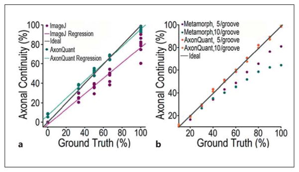
Comparison between AxonQuant and ImageJ or MetaMorph in quantifying axonal morphology. a Twenty-five microgrooves in which the axon density was sufficiently low to allow manual annotation as the ground truth were selected to compare the performance of AxonQuant with that of ImageJ. The linear regression of the results obtained using AxonQuant (green line) is closer to the ideal line than the one obtained by ImageJ (purple). In addition, the variation by AxonQuant is smaller than that by ImageJ. b Simulation data were used to compare the performance of AxonQuant with that of MetaMorph. AxonQuant shows better algorithm stability than MetaMorph. When the ground truth value for axonal continuity was high, the results obtained using MetaMorph showed more deviation and poorer linearity.

NeuronJ is a filament-tracking plug-in for ImageJ that was developed to measure neuronal morphology [12]. We compared our AxonQuant algorithm with ImageJ + NeuronJ, using 25 microgrooves in which the axon density was sufficiently low to allow manual annotation as the ground truth (fig. 7). For ImageJ, axonal continuity was determined by annotating all detectable continuous axons and calculating the total length of axons in the microgroove. All the quantification results by ImageJ are below the ideal line and have greater variation than those obtained by AxonQuant. This may be due to the fact that ImageJ does not allow precise annotation of all the axons because of axons overlapping or crossing over. The linear regression analysis indicates that our AxonQuant has better performance than ImageJ or NeuronJ (fig. 7). In addition, to quantify axonal continuity using ImageJ or MetaMorph is extremely time-consuming and often unreliable when axons are present at high density or cross each other or form bundles.

Discussion

In this study, we developed a microfluidic chamber-coupled axonal quantification algorithm that is suitable for high-throughput automatic quantification of axonal morphology. Under our culture conditions, embryonic cortical neurons harvested from one E18 pregnant rat (approx. 2.5 × 10⁶ cells), are sufficient for cultures in 50 microfluidic chambers, yielding 12,500 usable axonal bundles that can be imaged and quantified. The confocal imaging of 50 chambers takes approximately 25 h, and analyses of these images using our algorithm take no more than 0.5 h. Therefore, quantification of axonal morphology using our method is significantly more time efficient as compared with previously published methods.

In contrast to the traditional method using neurons cultured on coverslips, in which cell density and axonal density have a significant impact on the quality of axonal analysis, our microfluidic chamber-coupled AxonQuant method can be used at different cell densities with the analyses not affected by cellular or axonal density. In traditional neuronal cultures, when the cell density or axonal density is high or uneven, quantitative analysis of axonal morphology is often difficult. Furthermore, because of the small fraction of axons that can be selected for analyses by the traditional culture method and due to the inefficient nature of manual selection and manual analysis of axonal morphology, the traditional method of axonal quantification has been highly labor-intensive and fraught with selection bias as well as subjectivity in assessment.

In summary, our microfluidic chamber culture-coupled AxonQuant algorithm has several advantages over published methods [6–12] for axonal morphological analysis. First, our method allows efficient analyses of a large number of axonal images in a nonbiased objective manner. Second, the AxonQuant algorithm is more reliable and not affected by cell density or axonal density in cultures, in contrast to currently available software such as MetaMorph, which was used in our previous study. Third, our method makes it easy to automatically quantify large numbers of axonal bundles without manual selection of areas of interest, whereas traditional methods such as MetaMorph and ImageJ are useful only with individual axons when they are imaged at densities sufficiently low to allow selection/marking of axonal regions to be quantified. To assess axonal continuity using MetaMorph or ImageJ is extremely time-consuming and often not reliable when axons are present at a high density or overlap each other or form bundles, and it is difficult to decide whether there is axonal breakage or not.

The core algorithms, feature extraction and ANN-based feature analyzer of the Axon-Quant can also be used to quantitatively study axons of neurons cultured on regular cover-slips after minor modifications have been made. It should be noted that our algorithm can be used for quantifying axons of neurons cultured in commercially available microfluidic devices such as the ones provided by Xona Microfluidics LLC. In addition, the algorithm can also be used to quantify the specified structural feature of images, such as aggregates or filamentous structures, in a high-throughput manner. When fully utilized, our new method will facilitate large-scale high-throughput screening of genetic factors and pharmacological compounds that alter axonal morphology. Our method should be highly useful for studying neurodegenerative diseases involving axonal damage and for developing therapeutic approaches to such debilitating health problems.

References

- 1.Terry RD, Masliah E, Salmon DP, Butters N, DeTeresa R, Hill R, Hansen LA, Katzman R. Physical basis of cognitive alterations in Alzheimer’s disease: synapse loss is the major correlate of cognitive impairment. Ann Neurol. 1991;30:572–580. doi: 10.1002/ana.410300410. [DOI] [PubMed] [Google Scholar]
- 2.Medana IM, Esiri MM. Axonal damage: a key predictor of outcome in human CNS diseases. Brain. 2003;126:515–530. doi: 10.1093/brain/awg061. [DOI] [PubMed] [Google Scholar]
- 3.Brettschneider J, Petzold A, Sussmuth SD, Ludolph AC, Tumani H. Axonal damage markers in cerebrospinal fluid are increased in ALS. Neurology. 2006;66:852–856. doi: 10.1212/01.wnl.0000203120.85850.54. [DOI] [PubMed] [Google Scholar]
- 4.Burke RE, O’Malley K. Axon degeneration in Parkinson’s disease. Exp Neurol. 2013;246:72–83. doi: 10.1016/j.expneurol.2012.01.011. [DOI] [PMC free article] [PubMed] [Google Scholar]
- 5.Adalbert R, Coleman MP. Axon pathology in age-related neurodegenerative disorders. Neuropathol Appl Neurobiol. 2012 doi: 10.1111/j.1365-2990.2012.01308.x. Epub ahead of print. [DOI] [PubMed] [Google Scholar]
- 6.Kilinc D, Peyrin JM, Soubeyre V, Magnifico S, Saias L, Viovy JL, Brugg B. Wallerian-like degeneration of central neurons after synchronized and geometrically registered mass axotomy in a three-compartmental microfluidic chip. Neurotox Res. 2011;19:149–161. doi: 10.1007/s12640-010-9152-8. [DOI] [PMC free article] [PubMed] [Google Scholar]
- 7.Chen YC, Lin YQ, Banerjee S, Venken K, Li J, Ismat A, Chen K, Duraine L, Bellen HJ, Bhat MA. Drosophila neuroligin 2 is required presynaptically and postsynaptically for proper synaptic differentiation and synaptic transmission. J Neurosci. 2012;32:16018–16030. doi: 10.1523/JNEUROSCI.1685-12.2012. [DOI] [PMC free article] [PubMed] [Google Scholar]
- 8.Park KJ, Grosso CA, Aubert I, Kaplan DR, Miller FD. p75NTR-dependent, myelin-mediated axonal degeneration regulates neural connectivity in the adult brain. Nat Neurosci. 2010;13:559–566. doi: 10.1038/nn.2513. [DOI] [PubMed] [Google Scholar]
- 9.El-Laithy K, Knorr M, Kas J, Bogdan M. Digital detection and analysis of branching and cell contacts in neural cell cultures. J Neurosci Methods. 2012;210:206–219. doi: 10.1016/j.jneumeth.2012.07.007. [DOI] [PubMed] [Google Scholar]
- 10.Fujita Y, Sato A, Yamashita T. Brimonidine promotes axon growth after optic nerve injury through Erk phosphorylation. Cell Death Dis. 2013;4:e763. doi: 10.1038/cddis.2013.298. [DOI] [PMC free article] [PubMed] [Google Scholar]
- 11.Haass-Koffler CL, Naeemuddin M, Bartlett SE. An analytical tool that quantifies cellular morphology changes from three-dimensional fluorescence images. J Vis Exp. 2012;66:e4233. doi: 10.3791/4233. [DOI] [PMC free article] [PubMed] [Google Scholar]
- 12.Meijering E. Neuron tracing in perspective. Cytometry A. 2010;77:693–704. doi: 10.1002/cyto.a.20895. [DOI] [PubMed] [Google Scholar]
- 13.Campenot RB, Walji AH, Draker DD. Effects of sphingosine, staurosporine, and phorbol ester on neurites of rat sympathetic neurons growing in compartmented cultures. J Neurosci. 1991;11:1126–1139. doi: 10.1523/JNEUROSCI.11-04-01126.1991. [DOI] [PMC free article] [PubMed] [Google Scholar]
- 14.Taylor AM, Rhee SW, Tu CH, Cribbs DH, Cotman CW, Jeon NL. Microfluidic multicompartment device for neuroscience research. Langmuir. 2003;19:1551–1556. doi: 10.1021/la026417v. [DOI] [PMC free article] [PubMed] [Google Scholar]
- 15.Taylor AM, Dieterich DC, Ito HT, Kim SA, Schuman EM. Microfluidic local perfusion chambers for the visualization and manipulation of synapses. Neuron. 2010;66:57–68. doi: 10.1016/j.neuron.2010.03.022. [DOI] [PMC free article] [PubMed] [Google Scholar]
- 16.Campenot RB. Local control of neurite development by nerve growth factor. Proc Natl Acad Sci USA. 1977;74:4516–4519. doi: 10.1073/pnas.74.10.4516. [DOI] [PMC free article] [PubMed] [Google Scholar]
- 17.Campenot RB. Development of sympathetic neurons in compartmentalized cultures. I. Local control of neurite growth by nerve growth factor. Dev Biol. 1982;93:1–12. doi: 10.1016/0012-1606(82)90232-9. [DOI] [PubMed] [Google Scholar]
- 18.Campenot RB. Development of sympathetic neurons in compartmentalized cultures. II. Local control of neurite survival by nerve growth factor. Dev Biol. 1982;93:13–21. doi: 10.1016/0012-1606(82)90233-0. [DOI] [PubMed] [Google Scholar]
- 19.Millet LJ, Gillette MU. Over a century of neuron culture: from the hanging drop to microfluidic devices. Yale J Biol Med. 2012;85:501–521. [PMC free article] [PubMed] [Google Scholar]
- 20.Hanson L, Cui L, Xie C, Cui B. A microfluidic positioning chamber for long-term live-cell imaging. Microsc Res Tech. 2011;74:496–501. doi: 10.1002/jemt.20937. [DOI] [PMC free article] [PubMed] [Google Scholar]
- 21.Zhang K, Osakada Y, Xie W, Cui B. Automated image analysis for tracking cargo transport in axons. Microsc Res Tech. 2011;74:605–613. doi: 10.1002/jemt.20934. [DOI] [PMC free article] [PubMed] [Google Scholar]
- 22.Cusack CL, Swahari V, Hampton Henley W, Michael Ramsey J, Deshmukh M. Distinct pathways mediate axon degeneration during apoptosis and axon-specific pruning. Nat Commun. 2013;4:1876. doi: 10.1038/ncomms2910. [DOI] [PMC free article] [PubMed] [Google Scholar]
- 23.Whitesides G, Ostuni E, Takayama S, Jiang X, Ingber D. Soft lithography in biology and biochemistry. Annu Rev Biomed Eng. 2001;3:335–373. doi: 10.1146/annurev.bioeng.3.1.335. [DOI] [PubMed] [Google Scholar]
- 24.Ding J, Allen E, Wang W, Valle A, Wu C, Nardine T, Cui B, Yi J, Taylor A, Jeon NL, Chu S, So Y, Vogel H, Tolwani R, Mobley W, Yang Y. Gene targeting of GAN in mouse causes a toxic accumulation of microtubule-associated protein 8 and impaired retrograde axonal transport. Hum Mol Genet. 2006;15:1451–1463. doi: 10.1093/hmg/ddl069. [DOI] [PubMed] [Google Scholar]
- 25.Rosenblatt F. The perceptron: a probabilistic model for information storage and organization in the brain. Psychol Rev. 1958;65:386–408. doi: 10.1037/h0042519. [DOI] [PubMed] [Google Scholar]
- 26.Su KH, Wu LC, Lee JS, Liu RS, Chen JC. A novel method to improve image quality for 2-D small animal PET reconstruction by correcting a Monte Carlo-simulated system matrix using an artificial neural network. IEEE Trans Nucl Sci. 2009;56:704–714. [Google Scholar]
- 27.Do MN, Vetterli M. The finite ridgelet transform for image representation. IEEE Trans Image Process. 2003;12:16–28. doi: 10.1109/TIP.2002.806252. [DOI] [PubMed] [Google Scholar]
- 28.Charalampidis D, Kasparis T. Wavelet-based rotational invariant roughness features for texture classification and segmentation. IEEE Trans Image Process. 2002;11:825–837. doi: 10.1109/TIP.2002.801117. [DOI] [PubMed] [Google Scholar]
- 29.Yuan H, Zhang XP. Statistical modeling in the wavelet domain for compact feature extraction and similarity measure of images. IEEE Trans Circuits System Video Tech. 2010;20:439–445. [Google Scholar]
- 30.Chartier S, Boukadoum M, Amiri M. BAM learning of nonlinearly separable tasks by using an asymmetrical output function and reinforcement learning. IEEE Trans Neural Netw. 2009;20:1281–1292. doi: 10.1109/TNN.2009.2023120. [DOI] [PubMed] [Google Scholar]
- 31.Stanwood GD, Leitch DB, Savchenko V, Wu J, Fitsanakis VA, Anderson DJ, Stankowski JN, Aschner M, McLaughlin B. Manganese exposure is cytotoxic and alters dopaminergic and GABAergic neurons within the basal ganglia. J Neurochem. 2009;110:378–389. doi: 10.1111/j.1471-4159.2009.06145.x. [DOI] [PMC free article] [PubMed] [Google Scholar]
- 32.Basbaum CB. Induced hypothermia in peripheral nerve: electron microscopic and electrophysiological observations. J Neurocytol. 1973;2:171–187. doi: 10.1007/BF01474719. [DOI] [PubMed] [Google Scholar]
- 33.Kennett RP, Gilliatt RW. Nerve conduction studies in experimental non-freezing cold injury. I. Local nerve cooling. Muscle Nerve. 1991;14:553–562. doi: 10.1002/mus.880140610. [DOI] [PubMed] [Google Scholar]
- 34.Hoogeveen JF, Troost D, van der Kracht AH, Wondergem J, Haveman J, Gonzalez Gonzalez D. Ultrastructural changes in the rat sciatic nerve after local hyperthermia. Int J Hyperthermia. 1993;9:723–730. doi: 10.3109/02656739309032059. [DOI] [PubMed] [Google Scholar]
Associated Data
This section collects any data citations, data availability statements, or supplementary materials included in this article.