Generative models of rich clubs in Hebbian neuronal networks and large-scale human brain networks

Abstract

Rich clubs arise when nodes that are ‘rich’ in connections also form an elite, densely connected ‘club’. In brain networks, rich clubs incur high physical connection costs but also appear to be especially valuable to brain function. However, little is known about the selection pressures that drive their formation. Here, we take two complementary approaches to this question: firstly we show, using generative modelling, that the emergence of rich clubs in large-scale human brain networks can be driven by an economic trade-off between connection costs and a second, competing topological term. Secondly we show, using simulated neural networks, that Hebbian learning rules also drive the emergence of rich clubs at the microscopic level, and that the prominence of these features increases with learning time. These results suggest that Hebbian learning may provide a neuronal mechanism for the selection of complex features such as rich clubs. The neural networks that we investigate are explicitly Hebbian, and we argue that the topological term in our model of large-scale brain connectivity may represent an analogous connection rule. This putative link between learning and rich clubs is also consistent with predictions that integrative aspects of brain network organization are especially important for adaptive behaviour.

1. Introduction

The human brain can be viewed as a network, both at the macroscopic level of large-scale connections between brain regions and at the microscopic level of synaptic connectivity between billions of brain cells. In each case, the brain is conceived of as a collection of nodes (macroscopic brain regions or microscopic neurons) connected by links (figure 1a). The arrangement of these links, or the topology of these networks, is key to the system's overall function, much like the pattern of interactions between people is related to the spread of information across a social network [2,3].

Figure 1.

(a) Large-scale functional brain network adapted from [1]. The size of nodes encodes their degree (or number of connections), such that hubs are highlighted. The colour of each node encodes the module to which it belongs. (b) Schematic of a rich club. In this example, the degree threshold is three, so rich nodes (in red) are those nodes with a degree k > 3, and the rich edges (in black) are the five connections between them. The dashed black link indicates that a sixth connection could in principle exist within the rich club but is not realized, yielding a rich-club coefficient of Φ(k) = 5/6.

Interestingly, the past 20 years have seen an accumulation of evidence that both macro- and micro-scale brain networks as well as many other complex systems, from social networks to the Internet, display a range of topological properties in common [4]. For example, many systems will tend to be organized in modules with a high level of interaction within modules and sparser connectivity between them [5]. This separability of systems into quasi-independent units (such as departments within a company) has obvious operational advantages [6].

Another ubiquitous feature of network organization is the existence of highly connected nodes, or hubs (figure 1a), which often hold privileged positions of functional importance but are also points of vulnerability, as attacks targeting these nodes will lead to rapid disintegration of the system as a whole [7–10]. A more recent finding is that these hub nodes are not randomly distributed throughout the network, but instead tend to coalesce into an elite club of rich (highly connected) nodes [11,12]. These so-called rich-club structures have been observed in many systems, from social networks to power grids and most recently in brain networks [1,13]. Just like individual hubs have been shown to be central to a network's function, these rich-club structures are also particularly valuable to the overall function of the network [1,14].

An overarching idea emerging from such studies is that complex systems may be organized in similar ways because they were designed or have evolved to fulfil similar functions (such as efficient integration of information) under similar constraints (such as minimizing costs). In other words, the topology of complex systems can be thought of as the result of a cost–benefit analysis [15]. In spatially embedded networks, such as the human brain, physical connection costs tend to scale with the distance of these connections. Therefore, links tend to be short, and nodes in the same densely connected module tend to be co-localized in anatomical space. This is true at both the cellular level [16,17] and at the level of large-scale connections between brain regions [15].

The rich-club constitutes an exception to this rule as it is typically both densely connected and anatomically dispersed [1,13,18]. Rich clubs therefore incur high physical connection costs but this is likely to be offset by their distinctive value to the overall function of the network. For example, it was found that the shortest paths for carrying information between any two points in the human brain network are often routed through the rich club [1,14,18].

While the evolutionary logic behind this economical trade-off hypothesis is obvious, it is difficult to test directly in large-scale human brain networks. However, recent work has provided convergent evidence of similar rich-club structures in the cat cortex [19] and in the neuronal network of the roundworm, C. elegans [14]. The latter is the only organism for which the exact pattern of connections between neurons has been completely mapped [20], and laser ablation studies of individual neurons have assigned functional roles to most neurons in the animal. Interestingly, the network analysis in this model system revealed the existence of a high-cost, high-value rich club. Indeed, it contained a disproportionate amount of long-range connections (incurring high cost), while the nodes of the rich club corresponded to the set of command interneurons controlling forward and backward motion (a capability which is undoubtedly of high adaptive value to the organism) [14]. Given these observations on the existence and potential evolutionary advantage conferred by rich-club organization in brain networks at multiple scales, we asked the question: what set of generative factors could explain their formation?

Here, we take two complementary approaches: firstly, we consider generative models for the probability of a functional connection (an edge) between two cortical regions (nodes) separated by a given distance in anatomical space. In particular, we show that the emergence of rich clubs in large-scale human brain networks can be driven by an economic trade-off in which distance-dependent connection costs are balanced by a second term that favours network clustering. Interestingly, this economic clustering model has previously been shown to capture a range of other properties of human brain functional networks [21]. Secondly we show, using simulated neuronal networks, that Hebbian learning rules instantiated at the microscopic level also drive the emergence of rich clubs; and, furthermore, we find that the prominence of these features increases with learning time.

2. Material and methods

(a). Rich-club coefficient and other network measures

The rich-club organization of a network refers to nodes with high degree (or number of links), connecting to each other to form a club (figure 1b). Rich clubs are defined with respect to a threshold in degree, k, such that all nodes in the network with degree less than k are first removed and only the remaining subgraph is considered. The rich-club coefficient Φ(k) is then the ratio between the number of existing connections among the remaining rich nodes and the total number of possible connections that could exist between these nodes [11,12]

2.1

where N_k is the number of nodes with degree more than k and M_k is the number of edges between them. The computation of Φ(k) for all values of k in the network of interest yields a rich-club curve. Note, however, that hubs have a high probability of connecting to each other simply by chance, so even random networks generate monotonically increasing rich-club curves. To control for this effect, rich-club coefficients are normalized in the following way: Φ_norm(k) = Φ(k)/Φ_random(k), where Φ_random(k) is the average value of Φ(k) across 1000 comparable random networks generated by performing multiple double edge swaps on the original graph [22]. This procedure shuffles the links in the graph but preserves the degree of all nodes in the network (including the hubs). The existence of rich-club organization is then defined by Φ_norm(k) > 1 over some range of values of k. The significance level at each value of k is computed by counting the fraction of randomized controls, where Φ_random(k) > Φ(k) and a Bonferroni correction is used to control for multiple tests, yielding corrected p-values p_corr.

In this paper, we introduce the integrated rich-club coefficient to measure the extent of the rich club over the full range of k with a single scalar value. We define the integrated rich-club coefficient as the area between the Φ_norm(k) curve and the flat line at unit height, which is obtained by summing (Φ_norm(k) − 1) over all values of k ranging from unity to the maximum degree k in the network.

The clustering coefficient is defined as the number of triangular connections between a node's nearest neighbours divided by the maximal possible number of such triangular motifs. The overall clustering coefficient of the graph G is defined as the average clustering coefficient of all nodes i

2.2

The minimum path length (L_ij) between two nodes i and j is simply the minimum number of edges that need to be traversed to get from node i to j.

The nodal efficiency of a node i is defined as the inverse of the mean of the minimum path length between i and all other nodes in the network [23]

2.3

where N is the number of nodes in the graph. The global efficiency of the whole network E(G) is simply the average of all nodal efficiencies. Networks for which the average minimum path length between nodes is small can thus be said to have high global efficiency [23].

The betweenness centrality of a node i measures the fraction of shortest paths between any two nodes in the network that pass through i [24,25].

Many complex networks have a modular community structure, whereby they contain subsets of highly interconnected nodes called modules. The modularity Q(G) of a graph quantifies the quality of a suggested partition of the network into modules by measuring the fraction of the network's edges that fall inside modules compared to the expected value of this fraction if edges were distributed at random [25]. A graph can therefore be partitioned into modules by maximizing the value, Q(G), of the modularity across partitions of the graph [26]. Once this partition is obtained, we can calculate the participation coefficient of each node as a measure of its inter-modular connectivity

2.4

where is the intra-modular degree of node i in module S, and k_i is its total degree [27]. P(i) is close to unity if the node's links are uniformly distributed among all the modules and zero if all its links are within its own module.

(b). Large-scale brain network models

Large-scale brain functional networks are derived from resting state functional MRI (fMRI) data, which measures low-frequency neurophysiological oscillations at each of N cortical brain regions (nodes) in a group of volunteers. The functional connectivity between each pair of these regions can be estimated by the correlation between each pair of regional fMRI time series. Brain regions that have correlated time-series activity are said to be functionally connected. The resulting association matrix or functional connectivity matrix is thresholded to generate a binary, undirected network with arbitrary connection density [2].

The large-scale generative models of brain functional networks investigated here are those previously described in detail in [21]. Briefly, we build model networks by starting with 140 nodes corresponding to distinct cortical regions of the right hemisphere. Given the known anatomical locations of these nodes, the distance between each pair of nodes can be calculated. Edges are then placed in the network one by one. At each step, the position of the next edge is determined by calculating the probability of each potential edge based on the simple connectivity rules corresponding to the chosen model (equations (3.1)–(3.3)) and then drawing an edge at random, weighted by these probabilities. The procedure ends when a fixed number of edges has been reached, matching the number of edges in the observed brain functional networks to be modelled (after thresholding). Note that the resulting networks were slightly adjusted as in [21] to ensure none of the nodes were disconnected from the rest of the network. This was done for consistency with earlier work and does not influence the results reported here. The optimal parameters used for each model were also those published in [21], where simulated annealing was used to find the parameter setting that best fitted the data derived from fMRI measurements on 20 healthy volunteers. Finally, the resulting model networks can be analysed for features known to exist in real-world brain functional networks, such as the existence and characteristics of rich clubs within them.

(c). Neuronal network models

At the microscopic level, the cortex can be viewed as a large network of neurons, some of which are connected to each other via directed links along which signals (or spikes) can propagate. Neurons typically require strong external input, or the convergence of several inputs from other neurons in order to fire a spike. The aim of neuronal network models is to simulate the electrophysiological activity of neurons in response to both (modelled) external inputs and the signal received from neighbouring neurons as a result of overall activity.

Here, we use N = 1000 neurons, each modelled using the Izhikevich equations [28] which describe how a neuron's membrane potential v varies in time as a function of its past value and the inputs it receives. Once it reaches a certain threshold the neuron's membrane potential exhibits a sharp spike and this signal is transmitted as input to downstream neurons. The neuron's membrane potential is then reset to a baseline value until incoming stimuli drive it above threshold once more.

Here, as in [29], the parameters were set so that 80% of neurons modelled are excitatory and 20% are inhibitory, preserving the ratio found in the mammalian neocortex [30]. Each synapse, or connection, between a pair of neurons is characterized by a weight describing the contribution of the first (presynaptic) neuron's spikes to the membrane potential of the second (postsynaptic) neuron. Biologically, this corresponds to the type and amount of neurotransmitter released as well as the number of receptors available. We begin with every excitatory and inhibitory synaptic weight set to s = 6 and s = −5, respectively. Crucially, the excitatory synaptic weights assigned to each link change with time [31] following specific learning rules. Here, as in [29,32], we model learning with the (biologically realistic) additive spike-timing dependent plasticity rule described in [33], while inhibitory synaptic links are kept constant. In addition, synaptic weights were clipped at a maximal value of 10 mV implying that at least two simultaneous incoming spikes are necessary to drive a postsynaptic neuron to fire [29]. Our model also takes into account the existence of axonal conduction delays. These are modelled to be constant in time and randomly chosen integer values between 1 and 5 ms for excitatory neurons; inhibitory neurons all have 1 ms delays [29].

The rules we adopt for defining the connectivity of these artificial neural networks are as follows [29,32]: self-links and repeated links were excluded. Inhibitory neurons were only allowed to connect to excitatory neurons and the number of connections per neuron was set at k = 100. Following [32], the pattern of connections was slightly adapted from the one-dimensional Watts–Strogatz (WS) model [34], the first and simplest small-world network model ever proposed. In the original WS model, nodes are aligned along the perimeter of a circle and each node is linked to its k nearest neighbours (k/2 in each direction). This regular pattern of connections is then relaxed through the random rewiring of a proportion β of the existing links, to transform the regular lattice into a small-world network [34]. Here, we follow the same procedure, but the excitatory and inhibitory neurons are aligned along separate, concentric circles as sketched in figure 2 and described in [32]. All data presented use β = 0.4. This initial network topology changes over the course of the simulation as the weights of the connections evolve and certain links which reach zero weight are effectively removed.

Figure 2.

Schematic of links between excitatory and inhibitory nodes. Excitatory nodes (in blue) are arranged on the outer circle, while inhibitory nodes (grey) are on the inner circle. Each excitatory node is connected to its 80 neighbouring excitatory nodes (not shown). In addition, (a) each excitatory node (such as the one highlighted in red) is connected to a pool of 20 adjacent inhibitory nodes on the inner circle (only five of these connections are shown, for clarity). (b) The next three excitatory neurons along the outer circle (shown in grey) are also linked to the same pool of inhibitory ones. But the fourth excitatory neuron will shift by one unit its pool of target inhibitory neurons, so that all inhibitory neurons receive the same number of connections. (c) Correspondingly, each inhibitory neuron is linked to a pool of 100 adjacent excitatory ones (only five of these connections are shown). (d) The next inhibitory neuron along the circle has its pool of excitatory targets shifted by four units.

Over the course of the simulation, we first provide random input by injecting 20 mV to a randomly selected neuron every millisecond for 4 h (model time). This is followed by a training period during which, in addition to this background noise, the network is presented with a coherent stimulus of excitatory neurons. This consists of consecutive stimulation of neurons 1–48 with 50 mV at times 1, 2, … , 48 ms [29,32]. It has previously been shown that in response to such a stimulus the network reorganizes by altering the weight of connections so that some links effectively vanish while others are strengthened. As a result, subsequent presentation of the same stimulus triggers precise spatio-temporal patterns of activity uniquely associated with that input. In other words, the network has learnt to recognize the input stimulus. The resulting reconfigured networks can be analysed to see whether given features (such as a rich-club structure) also arise during learning.

3. Results

(a). Large-scale brain network models

In previous work, we compared several classes of generative models for the formation of large-scale brain functional networks [21]. Given the known anatomical location of the nodes in the network, we asked whether simple rules could predict the probability of functional connection between two cortical areas separated by some Euclidean distance in anatomical space.

The simplest (one-parameter) models specify that connection probability is a function only of distance between nodes [35,36]. The best-known model in this class is the exponential decay model where the probability of connection P_i,j between any pair of regions decays as an exponential function of the distance between them [35,36]:

3.1

where d_i,j is the anatomical distance between regions i and j, and η is the only parameter of the model. Varying η generates networks with variable degrees of cost penalization dictating the probability of connection between nodes.

We previously showed that cost penalization alone cannot simultaneously account for features such as the small-worldness, modularity and degree distribution of normal human brain functional networks. Given recent interest in rich clubs as key organizational features of brain networks, we are now interested in investigating whether this simple rule combined with the a priori node locations is enough to generate networks containing a rich club. Figure 3a shows that this is not the case, since no large hubs exist (maximum degree, k_max = 10), and the highest degree nodes are not preferentially linked to each other over and above what is expected by chance, or only minimally so, in just a fraction of model instantiations (see the electronic supplementary material, figure S1a).

Figure 3.

The rich club in model brain functional networks. (a) Exponential decay model, (b) economical preferential attachment model and (c) economical clustering model. For each model we show, on the left, the rich-club coefficient plotted against degree for a typical instance of the model network (in red) and for randomized versions of the network (average over randomized networks is shown in black, error bars show standard deviation, randomizations preserve degree distribution). The range of k-values over which the rich club is significant (p_corr < 0.05) is indicated with stars. On the right of each panel, we show a schematic of a typical network generated by the model (adapted from [21]), corresponding to the right hemisphere of a brain functional network—viewed from the top. The size of each node represents the degree of the corresponding brain region within the model network.

This finding is not surprising given that real-world rich clubs are known to contain many long-range links, which are exceptions to the cost minimization principle embodied in the exponential decay model. It therefore seems intuitive that a useful model requires a second term, balancing out the distance penalty term and allowing the emergence of longer connections and of highly connected hub nodes. One simple example is the economical preferential attachment (Eco PA) model, slightly modified from [37] to account for the fact that nodes are not added to the system one by one

3.2

Here P_i,j is the probability of connecting nodes i and j, of degree k_i and k_j, respectively, that are a distance d_i,j apart; η is the parameter of distance penalization, as before; γ is the parameter of preferential attachment (the exponent of a power law in the product of the degrees of the connected nodes). Intuitively, this model trades off the drive to shorter connection distance against the tendency to form highly connected hubs.

Figure 3b shows that, as expected, the Eco PA model both increases the prominence of hubs in the network and yields a rich-club regime, which is significant in most (90%) of model instances (see the electronic supplementary material, figure S1b). This is in line with previous results showing that the Eco PA model generated better approximations of brain networks than those simulated by cost penalization alone: the degree distribution was more realistically fat-tailed; global efficiency, clustering and modularity were all closer to their experimental benchmarks [21].

In terms of these basic topological properties, however, the best-fitting model previously identified was the economical clustering model which includes a negative bias against high connection cost, as before, and a positive bias in favour of consolidating connectivity between nodes having nearest neighbours in common. The probability of connection between two nodes i and j in this model is given by

3.3

where d_i,j is the anatomical distance between nodes i and j; k_i,j is the number of nearest neighbours in common between the nodes; η is the parameter of distance penalization; and γ is the topological clustering parameter. Large values of η decrease the probability of two distant nodes being connected, while larger values of γ increase the probability of connection between nodes that already have a large number of nearest neighbours in common. Figure 3c shows that the economical clustering model is able to generate highly significant rich-club structures over a broad range of degree thresholds k, and does so in a reliable manner (see the electronic supplementary material, figure S1c).

We note that the role of the clustering term controlled by γ in generating rich clubs may appear counterintuitive at first, since topological clustering is typically localized spatially and therefore competes in some sense against longer, more integrative connections. However, this local clustering emerges from a distance penalty alone. The parameter γ therefore controls the emergence of clustering among certain nodes despite the relatively large distance between them. It is this non-local clustering among hubs that favours the emergence of rich clubs.

Having established that simple economical trade-off models are able to generate rich clubs, we now consider whether these simulated networks also possess several other properties typically associated with rich-club organization in real-world brain networks. By selecting a particular degree threshold (k = 10) for further investigation, it is possible to partition the nodes and edges of a graph into the following categories: rich nodes, poor nodes, rich edges (linking two rich nodes), poor edges (linking two poor nodes) and feeder edges (linking a poor node to a rich one) (figure 4a). Using this classification, and independently of the degree threshold considered, both macro- and microscopic brain networks were empirically found to share the following features [14,18]: (i) rich nodes on average have significantly higher nodal efficiency, betweenness centrality, and participation coefficients than poor nodes; (ii) rich edges tend to span significantly longer distances than poor or feeder edges. Figure 4 shows that the rich clubs of model networks generated using the economical clustering model also share these properties. Similar results for 20 instances of the model and at various setting of the threshold K are reported in the electronic supplementary material. The significance of the results for a model instance, as shown in figure 4, can be estimated using permutation tests. For each metric shown, the difference in median value between rich and poor nodes (or edges in the case of distance) was compared to the difference obtained in a randomized network preserving the degree distribution, with the same number of rich nodes and edges selected at random. This resulted in the following significance values for each metric: degree p < 10⁻⁴, nodal efficiency p < 10⁻⁴, betweenness centrality p = 0.008, participation coefficient p = 0.048, distance p = 0.086. While this last p-value does not quite reach significance for a single model instance, it is important to note that the same pattern is observed for nearly all instances and across a range of K-values. Integrating over the range of K-values explored in the electronic supplementary material, for example, yields p = 0.051.

Figure 4.

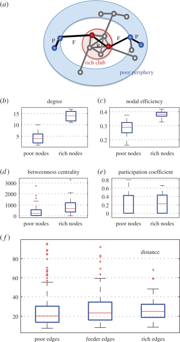
Properties of rich nodes and edges in brain networks. (a) Schematic of rich nodes (inside rich club) and poor nodes (in the periphery)—adapted from [14]. Edges connecting two poor nodes, two rich nodes and one rich node with one poor node are labelled P, R and F, respectively. Compared with poor nodes, rich nodes have (b) higher degree (by definition), (c) higher efficiency, (d) higher betweenness centrality and (e) higher participation coefficient. (f) The median length of rich edges is also higher than that of poor edges.

(b). Neuronal network models

Transmission of information between neurons occurs via the propagation of electrical impulses, called spikes (along the wiring) or axons (connecting different neurons). The strength of these connections is in turn influenced by the activity propagating on them. Here, we explore the conditions in which this plasticity might generate a rich-club structure in neuronal connections.

Our model comprised N = 1000 neurons, each modelled using the Izhikevich equations [28] as described in the §2c. Given that all nodes initially have degree k = 100 the initial network does not contain a rich club. However, the learning process will prune some of the edges as the network is trained with a given input stimulus. After a training period of T_train = 120 min (model time), we observe that a rich club has emerged (figure 5a).

Figure 5.

The rich club in neuronal networks. (a) Rich-club coefficient for a typical model network (in red) and for randomized networks preserving the degree distribution (average over randomized networks is shown in black, error bars show standard deviation). The range of k-values over which the rich club is significant (p_corr < 0.05) is indicated with stars. Compared with poor nodes, rich nodes have (b) higher degree (by definition), (c) higher efficiency, (d) higher betweenness centrality and (e) higher participation coefficient. (f) The integrated rich-club coefficient as a function of training time (red). The grey area shows 95% CIs based on 10 instances of the model at each value of training time.

Note that inhibitory nodes are disconnected from each other by definition and are constrained to stay at k = 100 since no learning takes place on inhibitory connections. For this reason, we have excluded inhibitory links from the rich-club analyses below. Note also that in order to consider the whole network, we have not excluded inhibitory nodes entirely, such that excitatory connections which connect to inhibitory neurons count towards these nodes' degree in our analyses. Considering only excitatory nodes and connections, however, yields a similar result, as shown in the electronic supplementary material, figure S2.

Considering the properties of the emergent neuronal rich club (at K = 60), we show in figure 5b–e that rich nodes again display higher efficiency, betweenness centrality and participation coefficient compared to poor nodes. The electronic supplementary material includes summary metrics capturing these results for 10 instances of the model and at various settings of the threshold K.

Once again, the significance of the results for a model instance as shown in figure 5 can be estimated using permutation tests. For each metric shown, the difference in median value between rich and poor nodes was compared to the difference obtained when selecting the same number of rich nodes and edges at random from the network. This resulted in the following significance values for each metric: degree p < 10⁻⁴, nodal efficiency p < 10⁻⁴, betweenness centrality p < 10⁻⁴, participation coefficient p = 6 × 10⁻⁴.

For consistency with previous work [29,32], we did not embed the neural network in physical space, so it is not possible to compare the distance of rich and poor edges in this context. Note that the characteristics of emerging rich clubs may also depend on the kind of stimulus used and on various parameter settings. We have followed the methods of [29,32], but investigating such dependencies will be the topic of further work. Here, we focus on a proof of principle that Hebbian learning is able to generate rich clubs in neuronal networks. To highlight this correspondence we show, in figure 5f, that the integrated rich-club coefficient increases sharply with training time before reaching a plateau after around 20 min.

4. Discussion and conclusion

In §3a, we explored a number of generative models to simulate the emergence of rich-club organization in large-scale brain functional networks. We have shown that the simplest models relying on distance penalty (or cost minimization) alone cannot account for the rich-club structures empirically observed. However, we found that the addition of a competing topological term to the model did give rise to robust rich clubs over a range of degree thresholds. This work extends our previous results which showed that such an economical trade-off model can simultaneously match many other network properties observed in fMRI data [21].

Rich clubs have attracted much attention over the past couple of years as key features of large-scale brain networks [38]. Their addition to the family of network properties accurately captured by the economical clustering model corroborates the importance of trade-offs between cost minimization and topological principles in the formation of brain networks. It also supports the idea that complex organizational structures such as rich clubs may be explicable in terms of a small number of biologically plausible generative factors, as in the one- and two-parameter models investigated in this study. For example, it is easy to imagine biological mechanisms which may enforce a distance penalty such as concentration gradients of growth factors directing axonal connections to target neurons [35,36]. In the preferential attachment model the second, topological, term is harder to link to known biological processes, as it requires global knowledge of the system including the identity of all the existing high-degree nodes [39]. The economical clustering model, on the other hand, relies only on local information. Furthermore, the enhanced probability of connection between nodes that already share nearest neighbours is at least conceptually compatible with Hebb's law, in the sense that neuronal groups that share common inputs from the same topologically neighbouring group are more likely to be simultaneously activated and therefore to consolidate direct functional connections [21].

To follow up on this intuition, we investigated, in §3b, whether simulated neuronal networks explicitly incorporating Hebbian learning rules (and implicitly incorporating a distance penalty) also develop rich-club structures, and reported for the first time that this is indeed the case. These results suggest the intriguing hypotheses that (i) rich-club structures might exist at all scales in the cortex, including the cellular scale for which connectivity data are currently unavailable, and (ii) the well-known process of Hebbian learning might mechanistically underpin the emergence of rich clubs in brain networks.

The degree to which Hebbian processes might play a role across different species and length scales is yet to be determined. In C. elegans, for example, the development of the rich club is not thought to be related to activity dependent plasticity. Instead, hub neurons are born early during development, before the worm begins to elongate [14]. The close proximity of the hub neurons at this early stage could allow for the formation of clustered connections among these hubs despite the large distances that will eventually separate them [40]. In humans, the development of large-scale brain networks is characterized by an initial phase of exuberant connectivity—or overproduction of axons, axonal branches and synapses—which is also thought to occur in an activity independent manner [41]. Hebbian mechanisms, however, are likely to play a role in the selection and reinforcement of permanent connections during the consolidation of both large-scale and small-scale cortical networks [41,42]. The degree to which these mechanisms contribute to the generation or strengthening of structural rich clubs at each scale is unknown.

Another question that requires further investigation is the relationship between the rich clubs observed in structural [13] and functional [1] brain networks. The large-scale networks modelled here were derived from correlational analysis of fMRI time-series data. However, such statistical evidence of functional connectivity between brain regions is not securely attributable to an underlying, direct anatomical connection. The impact of Hebbian processes at a synaptic level on large-scale functional connectivity remains to be explored experimentally.

To begin bridging these explanatory gaps, we first investigated whether the rich clubs generated in the large-scale and neuronal network models studied here share the characteristic properties that have been identified in empirical brain networks. We found that, indeed, all networks showed increased efficiency, betweenness centrality and participation coefficient in rich versus poor nodes. We then showed, in simulated neural networks, that the salience of rich-club features increases sharply with learning time (or duration for which a neural network undergoes Hebbian learning in response to a given stimulus). It is beyond the scope of this paper to explore the use of additional stimuli. We note, however, that previous experiments where these same neural networks were simultaneously trained with several stimuli allowed the performance of a network to be quantified in correctly recognizing each of the stimuli in a recall phase following Hebbian learning [21]. It was further shown that the quality of recall also increased with learning time at a similar rate as the rich club's salience does here [43].

These observations are significant for two reasons. Firstly, they further suggest a connection between the rich-club structure in neural networks, the mechanism through which it might emerge (Hebbian learning), and the function it might serve (efficient integration of information [44]). Secondly, they suggest testable hypotheses to motivate further investigation of the parallels between rich clubs at various scales and the potential role of Hebbian processes. One might expect, for example, that over the course of human development, periods during which cognitive capability is enhanced and Hebbian processes are particularly active may also correspond to increased salience of rich-club structures. This idea is supported by preliminary evidence from developmental neuroimaging studies which have revealed an increase in the number and importance of connector hubs in normally growing children and adolescents [45].

Finally, we note that this study raises a number of methodological questions. Firstly, the implementation of Hebbian learning in the neural network relies on pruning of connections (preferentially preserving clustering), while the Hebbian flavour of the economical clustering model results from the gradual addition of edges in a manner consistent with Hebbian principles (increasing clustering). This makes it difficult to compare directly trajectories of network properties over the course of learning or network growth between the models—a point that also needs careful consideration in future work comparing modelling results with developmental neuroimaging data. For this reason, it may be interesting to develop analogues of the economical clustering model based on the pruning of an over-connected initial network. Secondly, we note that, as in [21], the economical clustering model is applied here to a single hemisphere of the human brain. While this facilitates the approximation of the wiring length by the Euclidean distance between brain regions, we note that the rich clubs observed in human brain functional and structural networks most definitely span both hemispheres. More quantitative modelling of these rich clubs will therefore require addressing these and other issues surrounding the modelling of inter-hemispheric connections.

Funding statement

The Behavioural and Clinical Neuroscience Institute is supported by the Medical Research Council and the Wellcome Trust. P.E.V. is supported by the Medical Research Council (grant no. MR/K020706/1).

References

- 1.Crossley NA, Mechelli A, Vértes PE, Winton-Brown TT, Patel AX, Ginestet CE, McGuire P, Bullmore ET. 2013. Cognitive relevance of the community structure of the human brain functional coactivation network. Proc. Natl Acad. Sci. USA 110, 11 583–11 588. ( 10.1073/pnas.1220826110) [DOI] [PMC free article] [PubMed] [Google Scholar]
- 2.Bullmore E, Sporns O. 2009. Complex brain networks: graph theoretical analysis of structural and functional systems. Nat. Rev. Neurosci. 10, 186–198. ( 10.1038/nrn2575) [DOI] [PubMed] [Google Scholar]
- 3.Milgram S. 1967. The small world problem. Psychol. Today 2, 60–67. [Google Scholar]
- 4.Costa LDF, Oliveira ON, Jr, Travieso G, Rodrigues FA, Villas Boas PR, Antiqueira L, Palhares Viana M, Correa Rocha LE. 2011. Analyzing and modeling real-world phenomena with complex networks: a survey of applications. Adv. Phys. 60, 329–412. ( 10.1080/00018732.2011.572452) [DOI] [Google Scholar]
- 5.Girvan M, Newman MEJ. 2002. Community structure in social and biological networks. Proc. Natl Acad. Sci. USA 99, 7821–7826. ( 10.1073/pnas.122653799) [DOI] [PMC free article] [PubMed] [Google Scholar]
- 6.Simon HA. 1962. The architecture of complexity. Proc. Am. Phil. Soc. 106, 336–349. [Google Scholar]
- 7.de Solla Price DJ. 1965. Networks of scientific papers. Science 149, 510–515. ( 10.1126/science.149.3683.510) [DOI] [PubMed] [Google Scholar]
- 8.Barabási A-L, Albert R. 1999. Emergence of scaling in random networks. Science 286, 50–512. [DOI] [PubMed] [Google Scholar]
- 9.Albert R, Jeong H, Barabási A-L. 2000. Error and attack tolerance of complex networks. Nature 406, 378–382. ( 10.1038/35019019) [DOI] [PubMed] [Google Scholar]
- 10.Holme P, Kim BJ, Yoon CN, Han SK. 2002. Attack vulnerability of complex networks. Phys. Rev. E 65, 056109 ( 10.1103/PhysRevE.65.056109) [DOI] [PubMed] [Google Scholar]
- 11.Zhou S, Mondragón RJ. 2004. The rich-club phenomenon in the Internet topology. IEEE Commun. Lett. 8, 80–182. ( 10.1109/LCOMM.2004.823426) [DOI] [Google Scholar]
- 12.Colizza F, Flammini A, Serrano MA, Vespignani A. 2006. Detecting rich-club ordering in complex networks. Nat. Phys. 2, 110–115. ( 10.1038/nphys209) [DOI] [Google Scholar]
- 13.van den Heuvel M, Sporns O. 2011. Rich-club organization of the human connectome. J. Neurosci. 31, 15 775–15 786. ( 10.1523/JNEUROSCI.3539-11.2011) [DOI] [PMC free article] [PubMed] [Google Scholar]
- 14.Towlson EK, Vértes PE, Ahnert SE, Schafer WR, Bullmore ET. 2013. The rich-club organization of the C. elegans neuronal connectome. J. Neurosci. 33, 12 929–12 939. ( 10.1523/JNEUROSCI.3784-12.2013) [DOI] [PMC free article] [PubMed] [Google Scholar]
- 15.Bullmore E, Sporns O. 2012. The economy of brain network organization. Nat. Rev. Neurosci. 13, 467–482. [DOI] [PubMed] [Google Scholar]
- 16.Chen BL, Hall DH, Chklovskii DB. 2006. Wiring optimization can relate neuronal structure and function. Proc. Natl Acad. Sci. USA 103, 4723–4728. ( 10.1073/pnas.0506806103) [DOI] [PMC free article] [PubMed] [Google Scholar]
- 17.Niven JE, Laughlin SB. 2008. Energy limitation as a selective pressure on the evolution of nervous systems. J. Exp. Biol. 211, 1792–804. ( 10.1242/jeb.017574) [DOI] [PubMed] [Google Scholar]
- 18.van den Heuvel MP, Kahn RS, Goñi J, Sporns O. 2012. High-cost, high-capacity backbone for global brain communication. Proc. Natl Acad. Sci. USA 109, 11 372–11 377. ( 10.1073/pnas.1203593109) [DOI] [PMC free article] [PubMed] [Google Scholar]
- 19.de Reus MA, van den Heuvel MP. 2013. Rich-club organization of the human connectome. J. Neurosci. 33, 12 929–12 939. ( 10.1523/JNEUROSCI.1448-13.2013) [DOI] [PMC free article] [PubMed] [Google Scholar]
- 20.White JG, Southgate E, Thomson JN, Brenner S. 1986. The structure of the nervous system of the nematode Caenorhabditis elegans. Phil. Trans. R. Soc. Lond. B 314, 1–340. ( 10.1098/rstb.1986.0056) [DOI] [PubMed] [Google Scholar]
- 21.Vértes PE, Alexander-Bloch AF, Gogtay N, Giedd JN, Rapoport JL, Bullmore ET. 2012. Simple models of human brain functional networks. Proc. Natl Acad. Sci. USA 109, 5868–5873. ( 10.1073/pnas.1111738109) [DOI] [PMC free article] [PubMed] [Google Scholar]
- 22.Rubinov M, Sporns O. 2010. Complex network measures of brain connectivity: uses and interpretations. Neuroimage 52, 1059–1069. ( 10.1016/j.neuroimage.2009.10.003) [DOI] [PubMed] [Google Scholar]
- 23.Latora V, Marchiori M. 2001. Efficient behaviour of small-world networks. Phys. Rev. Lett. 87, 198701 ( 10.1103/PhysRevLett.87.198701) [DOI] [PubMed] [Google Scholar]
- 24.Freeman LC. 1977. Set of measures of centrality based on betweenness. Sociometry 40, 35–41. ( 10.2307/3033543) [DOI] [Google Scholar]
- 25.Newman MEJ. 2004. Fast algorithm for detecting community structure in networks. Phys. Rev. E 69, 066133 ( 10.1103/PhysRevE.69.066133) [DOI] [PubMed] [Google Scholar]
- 26.Leicht EA, Newman MEJ. 2007. Community structure in directed networks. Phys. Rev. Lett. 100, 118703 ( 10.1103/PhysRevLett.100.118703) [DOI] [PubMed] [Google Scholar]
- 27.Guimerá R, Amaral LAN. 2005. Cartography of complex networks: modules and universal roles. J. Stat. Mech. 2005, 1–13. ( 10.1088/1742-5468/2005/02/P02001) [DOI] [PMC free article] [PubMed] [Google Scholar]
- 28.Izhikevich E. 2003. Simple model of spiking neurons. IEEE Trans. Neural Netw. 14, 1569–1572. ( 10.1109/TNN.2003.820440) [DOI] [PubMed] [Google Scholar]
- 29.Izhikevich E. 2006. Polychronization: computation with spikes. Neural Comput. 18, 245–282. ( 10.1162/089976606775093882) [DOI] [PubMed] [Google Scholar]
- 30.Braitenberg V, Schuz A. 1991. Anatomy of the cortex: statistics and geometry. Berlin, Germany: Springer. [Google Scholar]
- 31.Caporale N, Dan Y. 2008. Spike timing-dependent plasticity: a Hebbian learning rule. Annu. Rev. Neurosci. 31, 25–46. ( 10.1146/annurev.neuro.31.060407.125639) [DOI] [PubMed] [Google Scholar]
- 32.Vértes PE, Duke T. 2010. Effect of network topology on temporal encoding in networks of spiking neurons. HFSP J. 4, 153–163. ( 10.2976/1.3386761) [DOI] [PMC free article] [PubMed] [Google Scholar]
- 33.Song S, Miller KD, Abbott LF. 2000. Competitive Hebbian learning through spike-timing-dependent synaptic plasticity. Nat. Neurosci. 3, 919–926. ( 10.1038/78829) [DOI] [PubMed] [Google Scholar]
- 34.Watts DJ, Strogatz SH. 1998. Collective dynamics of small-world networks. Nature 393, 440–442. ( 10.1038/30918) [DOI] [PubMed] [Google Scholar]
- 35.Kaiser M, Hilgetag CC. 2004. Spatial growth of real-world networks. Phys. Rev. E 69, 036103 ( 10.1103/PhysRevE.69.036103) [DOI] [PubMed] [Google Scholar]
- 36.Kaiser M, Hilgetag CC. 2004. Modelling the development of cortical networks. Neurocomputing 58, 297–302. ( 10.1016/j.neucom.2004.01.059) [DOI] [Google Scholar]
- 37.Yook SH, Jeong H, Barabási A-L. 2002. Modeling the internet's large-scale topology. Proc. Natl Acad. Sci. USA 99, 13 382–13 386. ( 10.1073/pnas.172501399) [DOI] [PMC free article] [PubMed] [Google Scholar]
- 38.van den Heuvel MP, Sporns O, Collin G, Scheewe T, Mandi RC, Cahn W, Goñi J, Hulshoff Pol HE, Kahn RS. 2013. Abnormal rich club organization and functional brain dynamics in schizophrenia. JAMA Psychiatry 70, 783–792. ( 10.1001/jamapsychiatry.2013.1328) [DOI] [PubMed] [Google Scholar]
- 39.Papadopoulos F, Kitsak M, Serrano M, Boguña M, Krioukov D. 2004. Popularity versus similarity in growing networks. Nature 489, 537–540. ( 10.1038/nature11459) [DOI] [PubMed] [Google Scholar]
- 40.Nicosia V, Vértes PE, Schafer WR, Latora V, Bullmore ET. 2013. Phase transition in the economically modeled growth of a cellular nervous system. Proc. Natl Acad. Sci. USA 110, 7880–7885. ( 10.1073/pnas.1300753110) [DOI] [PMC free article] [PubMed] [Google Scholar]
- 41.Innocenti GM, Price DJ. 2005. Exuberance in the development of cortical networks. Nat. Rev. Neurosci. 6, 955–965. ( 10.1038/nrn1790) [DOI] [PubMed] [Google Scholar]
- 42.Supekar K, Musen M, Menon V. 2009. Development of large-scale functional brain networks in children. PLoS Biol. 7, e1000157 ( 10.1371/journal.pbio.1000157) [DOI] [PMC free article] [PubMed] [Google Scholar]
- 43.Vértes PE. 2010. Computation in spiking neural networks, PhD thesis, p. 101 University of Cambridge, Cambridge, UK. [Google Scholar]
- 44.van den Heuvel MP, Sporns O. 2013. An anatomical substrate for integration among functional networks in human cortex. J. Neurosci. 33, 14 489–14 500. ( 10.1523/JNEUROSCI.2128-13.2013) [DOI] [PMC free article] [PubMed] [Google Scholar]
- 45.Khundrakpam BS, et al. 2012. Developmental changes in organization of structural brain networks. Cereb. Cortex 2, 2072–2085. ( 10.1093/cercor/bhs187) [DOI] [PMC free article] [PubMed] [Google Scholar]
Associated Data
This section collects any data citations, data availability statements, or supplementary materials included in this article.