Abstract
Diffusion kurtosis imaging (DKI) is a new model in magnetic resonance imaging (MRI) characterizing restricted diffusion of water molecules in living tissues. We propose a method for fast estimation of the DKI parameters. These parameters –apparent diffusion coefficient (ADC) and apparent kurtosis coefficient (AKC) – are evaluated using an alternative iteration schema (AIS). This schema first roughly estimates a pair of ADC and AKC values from a subset of the DKI data acquired at 3 b-values. It then iteratively and alternately updates the ADC and AKC until they are converged. This approach employs the technique of linear least square fitting to minimize estimation error in each iteration. In addition to the common physical and biological constrains that set the upper and lower boundaries of the ADC and AKC values, we use a smoothing procedure to ensure that estimation is robust. Quantitative comparisons between our AIS methods and the conventional methods of unconstrained nonlinear least square (UNLS) using both synthetic and real data showed that our unconstrained AIS method can significantly accelerate the estimation procedure without compromising its accuracy, with the computational time for a DKI dataset successfully reduced to only one or two minutes. Moreover, the incorporation of the smoothing procedure using one of our AIS methods can significantly enhance the contrast of AKC maps and greatly improve the visibility of details in fine structures.
Keywords: Diffusion kurtosis imaging, Diffusion tensor imaging, Parameter estimation, Magnetic resonance imaging
1. Introduction
Diffusion tensor imaging (DTI) is a non-invasive technique for characterizing the motion of water molecules in living tissues [1]. It assumes that the random displacement of water molecules approximately follows a Gaussian distribution. Although DTI has been successfully applied in many neuroimaging studies, the assumption of a Gaussian distribution of motion is not strictly accurate because of the effects of tissue microstructure on the diffusion of water. New methods have been proposed to account for the non-Gaussian components of this diffusion, such as the Multi-Exponential model [2,3] or the q-space imaging technique. The Multi-Exponential model assumes that a single voxel may consist of multiple compartments, and diffusion in each compartment satisfies Gaussian model. The consolidated diffusions in all these compartments thus results in non-Gaussian phenomenon. In contrast, the q-space imaging technique makes no assumptions about the number of tissue compartments, but instead directly evaluates the displacement probability distribution function of water molecules [4,5].
Jensen and his colleagues recently proposed a new and efficient model, called diffusion kurtosis imaging (DKI) [6], for studying the non-Gaussian characteristics of water diffusion in tissue structures [7]. This model makes no assumption about the number of tissue compartments, and requires less scanning time (approximately 10 min) than does the q-space imaging. It introduced a kurtosis term into the expression of displacement distribution to evaluate the deviation from a Gaussian model. This kurtosis coefficient was then incorporated into a tensor model [8-10]. However, the kurtosis value could be over-estimated significantly in certain cases, and investigators have developed a method that uses a framework for estimation of constrained maximum likelihood (CML) with a Rician-noise model to prevent this from happening [11]. Anyway, compared to conventional DTI indices, the kurtosis value provides additional information of microstructure complexity in both white and gray matter, and is more sensitive to the presence of tissue heterogeneity [12-14]. Due to these advantages of the kurtosis term, DKI has been successfully applied to human studies on aging [15], attention deficit hyperactivity disorder [16], cerebral glioma [17], epilepsy [18], head and neck cancer [19], and animal models [20].
The DKI model uses conventional diffusion weighted imaging (DWI) data, but it requires data acquired with no less than 3 different b-values. The key parameters of the DKI model, including the apparent diffusion coefficient (ADC) and the apparent kurtosis coefficient (AKC), can be estimated using an unconstrained nonlinear least squares (UNLS) method [6]. This method performs robustly but usually requires at least ten minutes to complete processing one single DKI dataset typically containing 30 slices acquired using 6 b-values along 30 gradient directions, which is excessively time consuming for clinical applications in practice. To shorten the processing time, Jensen et al. suggested directly solving the nonlinear function using 3 b-value data [21], which would allow a dataset to be evaluated in real time. Unfortunately, this method works only for cases of 3 b-values, and is therefore not a general solution. Recently, a new method, namely constrained linear least squares (CLLS), was proposed, achieving a fast speed of computation and comparatively better accuracy [22]. The CLLS method re-parameterizes the nonlinear function of DKI, and transforms it into a 2-variable linear problem. However, this approach needs to acquire data along more than 15 diffusion gradient directions to estimate ADC and AKC tensors, which therefore requires lengthy acquisition time.
We propose a method for rapid estimation of DKI parameters that uses an alternative iteration schema (AIS). It calculates ADC and AKC alternatively using a simple calculation formula and thus significantly reduces the calculation complexity. In addition, it adopts an iteration framework, which can easily incorporate extra constraints and smoothing procedures to improve the accuracy and robustness of the estimation. More specifically, the AIS method estimates ADC and AKC for each gradient direction independently, with each individual direction using data acquired at multiple b-values. In this algorithm, we first estimate initial values of the ADC and AKC using data acquired at baseline and two non-zero b-values from a DKI dataset. Second, we use an iterative framework to calculate these two parameters alternately until the results converge. Furthermore, we incorporate constraints and a smoothing procedure in each iteration to ensure the accuracy and robustness of the estimation (see the Method Section). Thus, we have evaluated three versions of the AIS method: the original or unconstrained AIS (UAIS, section 2.2), the constrained AIS (CAIS, section 2.3), and the smoothed and constrained AIS (SCAIS, section 2.4). In the evaluations, we used both synthetic and real data, against a number of other methods popularly in use. In a recent study on epilepsy [18], we successfully applied the proposed method to DKI data and achieved satisfactory results.
2. Method
In this section, we first briefly introduce the conventional UNLS method, discussing its high computational complexity due to the nonlinearity of DKI. Then we present an assumption on the nonlinear function that leads to an alternative iteration schema to simplify the calculation, thereby yielding the UAIS method. In addition, constraints and an additional smoothing procedure are subsequently incorporated into the iteration framework to improve the estimation accuracy and precision, resulting in the CAIS and SCAIS methods. Finally, an overview will be given to elaborate the algorithmic details of the AIS methods.
2.1 The UNLS Method
The DKI model containing the ADC and AKC terms is a nonlinear function:
| (1) |
in which D and K denote ADC and AKC, respectively, and b denotes the b-value. S(b) and S(0) are the signal intensity of DWI data and the baseline measurement without applying any diffusion gradient, respectively.
Conventional UNLS methods optimize ADC and AKC value simultaneously using nonlinear curve fitting [6]. The fitting procedure aims to minimize the Euclidean Norm of difference between S(bn)/S(0) and exp(-bn + 1/6 · bn2D2K), as shown below:
| (2) |
where N denotes the total number of b-values involved in nonlinear fitting, and n is the current index of b-value. In Eq. (2), the 2nd order term of b-value accounts for the main difference between the DKI and DTI models.
The Levenburg-Marquadt algorithm is commonly used to solve the minimization problem of the nonlinear cost function [23], namely Eq. (2). However, the calculation of this method needs iterations and requires a matrix inversion and partial derivatives in each iteration In addition, the parameters are normally estimated in a voxel-wise fashion. The computational burden is therefore very heavy for a DKI dataset because of the involvement of a large number of voxels.
In fact, logarithm can be applied to Eq. (1) for computational efficiency, thus the minimization turns to be log-nonlinear least squares fitting as follows:
| (3) |
where wn is a weight for DWI measurement of the nth b-value, and should be set as wn = S(bn)2 [24].
2.2 The UAIS Method
Considering that avoiding nonlinear fitting may significantly shorten computation time, we introduce as follows an iterative schema, i.e., the UAIS method, to update ADC and AKC alternatively and progressively. The nonlinear fitting thus degenerates into a process of linear fitting.
2.2.1 The Iteration Framework
Supposing that we want to calculate an updated ADC value from Eq. (3), while a current estimation of the ADC and AKC values have already been obtained from a previous step, thus the following equation should be satisfied:
| (4) |
where Ki denotes AKC calculated from the ith iteration (the previous iteration step), Di+1 is the new ADC value to be calculated and is the only unknown variable to be estimated in Eq. (4). However, Eq. (4) is a nonlinear function due to the 2nd order term of Di+1, which is hard to solve.
We further assume that the Di+1 in the 2nd order term can be approximated by Di. Consequently, the solution of Di+1 can be greatly simplified. We can do so because the terms “−bD+(1/6)×b2D2K” in Eq. (3) is essentially a Taylor expansion of ln[S(b)/S(0)] in the power of b[6] . The 2nd order term of b is theoretically much smaller than the 1st order term, thus estimation error introduced by replacing Di+1 with Di in the 2nd order term is comparatively small and can be ignored. Di+1 can thus be estimated simply using a linear least squares fitting with an explicit analytical solution as follows:
| (5) |
Now using this newly obtained ADC, we can derive the formula for estimation of AKC in a similar approach. Again, because AKC only contains linear term, Ki+1 also has an analytical solution:
| (6) |
In this iteration schema, ADC and AKC are updated alternatively at each step of the iteration. A new ADC can be calculated based on the latest values of ADC and AKC in the previous steps, and a new AKC can be subsequently updated via the currently calculated ADC. Consequently, the estimation will be alternatively repeated until no significant difference of both ADC and AKC values is observed between two consecutive iterations.
In contrast to the regular nonlinear fitting, the computational expense of our UAIS is much lower, although it employs the same cost function. This is because our UAIS method introduces a simple form of linear calculation in each iteration. The previous work [22] made an assumption that if the 2nd order term, D2K, can be treated as a linear variable independent of the 1st order term “D”, then the nonlinear DKI function can be re-parameterized into a two-variable linear problem, and the iteration will converge. In our work, we therefore approximate the 2nd order term linearly but in a different way. Taking the ADC and AKC in the 1st and 2nd order term respectively as two independent variables, we calculate them alternatively. Thus, in the calculation of ADC, we can approximate the 2nd order term using a pair of ADC and AKC values from a previous iteration which is based on Taylor expansion, so that the actual role of this 2nd order tem is simply similar to an independent 1st order term. Moreover, initializing ADC and AKC with descent accuracy (described in Section 2.2.2) will further guarantee that such approximation is feasible and practical. We thus can degenerate the nonlinear least squares function into linear least square functions of two variables. Mathematically, such a linear least squares problem is convex and always has a closed-form solution that is unique [25]. This property therefore guarantees that our iteration process converges.
2.2.2 Initialization
Now let us go back to the issue of how to initialize ADC and AKC values as the basis for starting the iterative process. The three-points technique proposed in [14] actually provided an efficient solution to this issue. It directly solves the DKI nonlinear equation, namely Eq. (1), using DKI dataset based on a subset of the DWI data that requires data at one baseline and two nonzero b-values. Thus, initial ADC D0 and initial AKC K0 can be estimated as follows:
| (7) |
where b1, b2 are the two nonzero b-values. D(1), D(2) are diffusion coefficients calculated by their individual DWI data at the corresponding b-value:
| (8) |
This initialization gives a nice approximation of ADC and AKC values that benefits the convergence process of our method. It also ensures the effectiveness of our approximation of the 2nd order term as outlined in the last section. Now, we have all the components for UAIS.
2.3 The CAIS Method
To ensure that the parameters are physically and biologically plausible, we apply constraints in every iteration step to the UAIS method, thereby making it CAIS. We know that ADC must be non-negative, which is also demanded by the conventional DTI model [14]. Although AKC can be either positive or negative [7], and in theory the feasible minimum of AKC is -2, multi-compartment diffusion models and empirical evidence in the brain suggest a super-Gaussian displacement distribution, indicating that the minimum of AKC should be zero but not -2 [26], therefore AKC has to be non-negative [22]. Moreover, S(b) is supposed to be a monotonically decreasing function of the b-value, and the upper boundary of AKC should be set as [14]:
| (9) |
2.4 The SCAIS Method
Although these constraints can well confine ADC and AKC within reasonable ranges, they sometimes are still vulnerable to estimation errors. The principle of the DKI model shows that the estimation of AKC strongly depends on the accuracy of ADC value. From Eq. (1), we derive the correlation between AKC and ADC as K = 6(ln(S/S0) + bD)/(b2D2). If the estimated ADC contains a small error εD (εD ≈0 or D + εD ≈ D), then the transferred error εk to AKC will be
| (10) |
As ADC values are usually in the scale of 1 μm2/ms, εK will be 2.4∼12.0 times as large as εD at b-value 500∼2500 s/mm2. For smaller ADC values, εK will be even larger. For example, if the true values of a voxel are ADC = 0.3 μm2/ms and AKC = 2, when noise or artifacts introduces an error εD = -0.1 μm2/ms, according Eq. (1), the estimated AKC is -3 at b-value = 2000 s/mm2. Although AKC will be constrained to be non-negative, zero is definitely not an acceptable result in this case.
To minimize the potential errors as alerted by Eq. (10), we further develop the CAIS method into the smoothed and constrained AIS (SCAIS) method, which estimates AKC using smoothed ADC in each iteration step. We simply adopt a 3D Gaussian filter within a 3×3×3 cubic neighborhood. To keep the original spatial resolution and avoid over-smoothing, the smoothing is not directly applied to ADC. Instead, we calculate a temporary version of the smoothed ADC map in every iteration only for AKC estimation.
2.5 Overview of the Iteration Schema
In brief, our ultimate alternative and iterative schema can be described as follows:
Initialize ADC and AKC
REPEAT
Update ADC
Apply ADC constraint
Smooth ADC and get an intermediate version of ADC ( for SCAIS only )
Update AKC
Apply AKC constraint
UNTIL convergence
3. Experiment
We compared our proposed methods with the conventional UNLS method using both synthetic data and real DKI data. In this comparison, the CLLS and CML methods were also considered. For a fair comparison, we modified the CLLS method to be capable of directly calculating ADC and AKC along each independent gradient direction but not using the tensor models. Moreover, the original CLLS method did not consider any weighting term as presented in Eq. (3). We thus examined both the original and the weighted versions of the CLLS methods (CLLS & WCLLS) in our experiments. The names and their abbreviations of all these methods are listed for readers' convenience (Table 1).
Table 1.
The list of methods for DKI estimation and their abbreviations used in this paper.
| Full name | Abbreviation |
|---|---|
| Constrained nonlinear least square / unconstrained nonlinear least square | CNLS / UNLS |
| Constrained linear least square / unconstrained linear least square | CLLS / ULLS |
| Weighted constrained linear least square / weighted unconstrained linear least square | WCLLS / WULLS |
| Constrained maximum likelihood / unconstrained maximum likelihood | CML / UML |
| Constrained alternative iteration schema / unconstrained alternative iteration schema | CAIS / UAIS |
| Smoothed and constrained alternative iteration schema / Smoothed and unconstrained alternative iteration schema | SCAIS / SUAIS |
For the algorithm parameters, we used Levenberg-Marquardt algorithm in the UNLS method and the initial ADC and AKC were set at 0 μm2/ms and 0. In the three versions of our method, namely UAIS, CAIS and SCAIS, we terminated the iteration processes whenever the updating differences of the estimated ADC and AKC values became less than 0.001 μm2/ms and 0.001, respectively. We used a subset of a complete DWI dataset with two nonzero b-values, including one near 800 s/mm2 and one at the maximal available (2600 s/mm2), to initialize the three AIS methods, which is based on our previous study that investigated the optimized DKI acquisition parameters and imaging schemas [27]. For the smoothing procedure in SCAIS, a Gaussian kernel with full width at half maximum (FWHM) of 1.5 pixels (σ = 0.64 pixel, as FWHM = 2 σ (2Ln2)1/2 ≈2.35482 σ) for synthetic data and 3 mm (σ ≈ 1.27 mm or 1.5 voxels) for real data was used for ADC smoothing. All these algorithms were implemented in Matlab (http://www.mathworks.com) on a Linux platform (CPU 1.0 GHz, Memory 8G).
3.1 Experimental Design
3.1.1 Synthetic Data for DKI Model
In the first experiment, we wanted to compare quantitatively the performance of our iteration schema with that of the conventional UNLS, CLLS, WCLLS, CML methods. Both constrained and unconstrained versions of these methods were compared.
A synthetic DWI dataset of 6 b-values (0∼2500 s/mm2) was constructed. This construction was a procedure reversing the process for parameter estimation. We first created a pair of 2D ADC and AKC maps. The map consisted of 9 columns, in which we set the values of the ADC and AKC pairs at (0.4, 2.0), (0.5, 1.8), (0.6, 1.5), (0.8, 1,2), (0.9, 1.0), (1.0, 0.9), (1.2, 0.8), (1.8, 0.6), (2.5, 0.4), based on statistics in human data [6]. The order of the columns is randomized to avoid smooth changes across the borders of the neighboring values in the phantom, which somehow simulated the structural presentation in real-world human data (Fig.1). Certainly, each pair of ADC and AKC satisfied the physical and biological constraints, as outlined in Eq. (9). We then used these ADC and AKC maps to calculate DWI data basing on Eq. (1), with the baseline signal intensity at 200. In the last step, we superimposed Rician noise to the synthetic DWI data to mimic the realistic noisy situation in an MRI system. Because Rician noise originates from independent Gaussian white noise in real and imaginary channels, we simulated the noise as follows:
Figure 1.
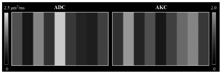
A synthetic DKI dataset before noise was superimposed. (Left) Apparent diffusion coefficient (ADC) maps; (Right) The corresponding apparent kurtosis coefficient (AKC) maps.
| (14) |
where I0 was the noise-free signal and IN the final noisy signal; and n was the Gaussian noise with zero mean and standard deviation (STD) σ. We added 5 levels of Rician noise with the STD ranging from 2 to 10 in both the real and imaginary channels. The corresponding signal-to-noise ratios (SNR) of the simulated DWI data were thus from 50 to 10.
The ADC and AKC maps were estimated from the currently simulated DWI data using each estimation method. For quantitative comparison, we evaluated the general quality of the estimated parameter maps using Root Mean Square Error (RMSE):
| (15) |
where Ω is a mask for region-of-interest (in this experiment, the mask simply covered the whole image), I denotes either the estimated ADC or the AKC map, and u is the corresponding reference map.
We further evaluated the effect of employing the smoothing procedure in our SCAIS by comparing it against the CAIS method, which differed only without using the smoothing procedure. We conducted the evaluation by inspecting their estimation bias (difference between estimated parameters and its ground truth) and variance of ADC and AKC, which treats the maps provided by the UNLS method as reference. We consider these two indices as a complement of RMSE, which would reflect the estimation accuracy and precision, respectively.
We also inspected the converging speed of our AIS and the conventional UNLS methods. We recorded after each iteration step the RMSE of the resulting ADC and AKC. The WCLLS/WULLS and CLLS/ULLS were not included in this comparison because they are not iterative methods.
Finally, we evaluated the impact of smoothing ADC on estimating AKC, which was only included in the SCAIS method. The FWHM of Gaussian kernel was set at five different levels, namely 0.5, 1.0, 1.5, 2.0, 3.0 voxels. To carefully examine the inaccuracy that could be propagated from the smoothing ADC to AKC, we calculated the residual maps in addition to quantitative comparisons of the RMSE values of AKC.
3.1.2 Synthetic Data for Bi-Exponential Model
To examine whether exactly the DKI parameters can be accurately estimated when diffusion deviates from Gaussian model, we created another synthetic dataset based on bi-exponential model for further evaluation of the performance of these DKI methods. Bi-exponential model assumed that a single voxel may consist of 2 compartments, and the diffusion signal decayed by formula S(b) = S(0) (λ exp(-bD1) + (1-λ) exp(-bD2)), where D1 and D2 are diffusion coefficients in the two compartments, and λ is a weighting factor of the first compartment.
We constructed the corresponding synthetic DWI dataset of 6 b-values (0∼2500s/mm2) with a procedure similar to that in the previous section. We first created two ADC maps, one has a fixed value of 0.5 μm2/ms, and the other contains ADC values increasing from 0.0 to 1.0 (increment 0.05) μm2/ms. λ was set at 0.5. We then calculated DWI data with a baseline signal intensity at 200, and added 5 levels of Rician noise to the DWI data (SNR from 10 to 50).
Again, we used RMSE values to quantify estimation error of ADC and AKC maps calculated by each of the methods. The maps calculated from noiseless DWI data using UNLS method were taken as the ground truth.
3.1.3 Real Data
In a third experiment, we evaluated the practical performance of our methods against the UNLS method using real-world human datasets. DKI data from five healthy volunteers were collected on a 3T Siemens Trio system at East China Normal University with their written consents and an approval from the local institutional review board (IRB). Each dataset contained one baseline and 11 DW images at non-zero b-values ranging from 600 to 2600 s/mm2 with an interval of 200 s/mm2. The maximum and minimum of b-values adopted here were similar to the recommended values in previous reports [6,9]. The other parameters were: 12 non-parallel diffusion gradient directions, number of excitation (NEX) = 2, TR = 5300 (3 participants) / 6100 (2 participants) ms, TE = 110 ms, matrix = 128×128, FOV = 256×256 (4 participants) / 230×230 (1 participant) mm2, slice thickness = 3mm with no gap, number of slice = 34 (3 participants) / 39 (2 participants) total scan time 22 min 53 sec (3 participants) / 27 min 22 sec (2 participants). (Note that the imaging parameters for the 5 participants were slightly different because these were the data collected in history for different research purposes. We did not redo data collection because we believe that the variations existing in the datasets could better serve our purpose for evaluating the performance of the methods under various conditions.) To minimize possible noise and artifacts, we acquired 8 extra baseline images so that we got a total of 10 baseline imaging data.
In the preprocessing steps, we first corrected all DWI data for eddy-current induced distortion using “eddy correct” toolbox of FSL (http://www.fmrib.ox.ac.uk/fsl/), and then routinely regularized using a 3D Gaussian kernel with FWHM = 3 mm [15,17,22]. Next, we averaged the 10 baselines and the 2 repetitions of the DWI images, respectively, after they were spatially coregistered.
A DKI dataset typically contains data acquired at 3 to 6 b-values. We thus constructed datasets with DWI data of 6, 5, 4 and 3 b-values (in short, 6b, 5b, 4b and 3b) extracted from the complete datasets (12 b-values) in a similar way as reported [27], which are commonly used configurations in real clinical studies. The b-values involved in these newly constructed individual datasets were nearly equally distributed (Table 2).
Table 2.
Estimation error (RMSE) and computational time of the conventional UNLS method and our proposed UAIS method when using DWI data of 3 to 6 b-values. The accuracy of our method was very similar to that of the conventional method, but our method is astonishingly faster than the UNLS method.
| Row | b-number | List of b-values (mm/s2) | UNLS | UAIS | ||||||||
|---|---|---|---|---|---|---|---|---|---|---|---|---|
|
| ||||||||||||
| RMSE | RMSE | Time | ||||||||||
|
|
|
|||||||||||
| ADC | AKC | ADC | AKC | |||||||||
| 1 | 6b | 0 | 600 | 1000 | 1600 | 2000 | 2600 | 0.0436 | 0.1055 | 0.0627 | 0.1079 | 116 s |
| 2 | 5b | 0 | 800 | 1400 | 2000 | 2600 | 0.0599 | 0.1285 | 0.0753 | 0.1288 | 97 s | |
| 3 | 4b | 0 | 800 | 1600 | 2600 | 0.0609 | 0.1419 | 0.0855 | 0.1423 | 64 s | ||
| 4 | 3b | 0 | 1000 | 2000 | – | – | 0.1048 | 0.2693 | 7 s | |||
We first quantitatively and visually compared our UAIS schema with the UNLS method, using subsets of the DWI data acquired at 4, 5 and 6 b-values. This test inspected how well the UAIS schema can approximate the UNLS method. Therefore, we calculated their RMSE values of the ADC and AKC maps for quantitative comparison, which again referenced the parameter maps estimated from the complete dataset by UNLS as for comparison. In addition, we also visually compared their corresponding mean diffusion (MD) and mean kurtosis (MK) maps (calculated by averaging ADC and AKC along all available gradient directions). Finally, we compared the convergence performance of the two methods. In this study using real data, we did not quantitatively compare the CAIS and SCAIS methods with UNLS because we will see in the first experiment that the SCAIS and CAIS methods may outperform the UNLS method due to the physical, biological constraints and smoothing procedure. We also visually compared CAIS and SCAIS methods on the AKC and MK maps.
3.2 Results
3.2.1 Synthetic Data for DKI Model
The results of the first experiment showed that our proposed AIS methods performed equally or better than the other methods. The RMSE values of ADC and AKC maps calculated from most of the methods were very close to each other, including the constrained methods such as CNLS, WCLLS, CML, CAIS, and their unconstrained version (Fig. 2), thus our CAIS and UAIS methods showed equivalent performance as other currently available methods. Furthermore, using the mentioned smoothing procedure, our SCAIS method achieved lower RMSE in AKC than other methods at every noise level (Fig. 2). In addition, we also found that the RMSE values of ADC using CLLS/ULLS were significantly higher than the other methods.
Figure 2.
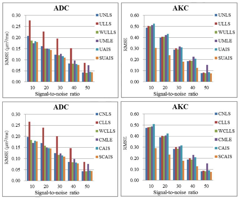
A RMSE (root mean square error) comparison of parameter estimation methods using synthetic DKI dataset. Five levels of noise were added. Estimation methods either without (upper) or with (lower) constraints were respectively compared. The RMSE of the resulting ADC (left) and AKC (right) maps showed that our three AIS methods (UAIS, CAIS and SCAIS) provided similar or better results compared to conventional methods. In particular, SCAIS performed the best. (Refer to Table 1 for abbreviations of the methods.)
The evaluation of estimation bias and variance showed that the smoothing procedure in SCAIS significantly improved both the estimation accuracy and precision of AKC (Fig. 3). For ADC, both SCAIS and CAIS methods achieved accurate results with very small estimation bias and variance around 0.01μm2/ms and 0.02, respectively (a typical ADC value is in the scale of 1.0 μm2/ms). Because the differences were almost hardly perceivable, they were not shown here.
Figure 3.
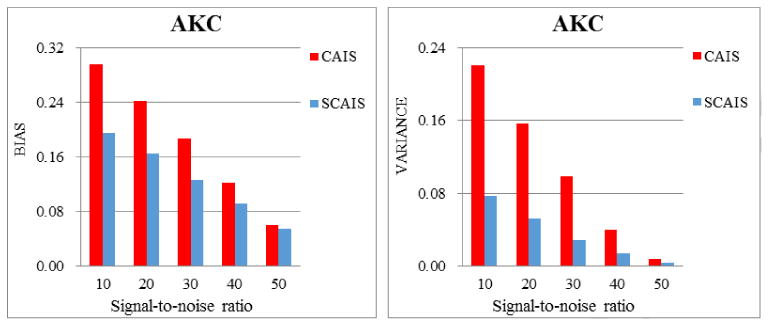
A comparison of estimation bias and variance for AKC using synthetic DKI dataset. (a) bias (difference between estimated map and the ground truth); (b) variance. Compared to CAIS, smoothing procedure in SCAIS significantly reduced both estimation bias and variance of AKC, thus achieved better estimation accuracy and precision.
Visual inspection of the ADC and AKC maps agreed with the analyses that the SCAIS was more robust than other methods under heavier noise for AKC, especially in the region of low ADC and high AKC (Fig. 4). We did not include CNLS, ULLS, WULLS/WCLLS, UML, UAIS and SUAIS methods in the visual comparison because we have seen in the previous RMSE analysis that these methods performed very similarly to that of UNLS, CLLS, CML and CAIS.
Figure 4.
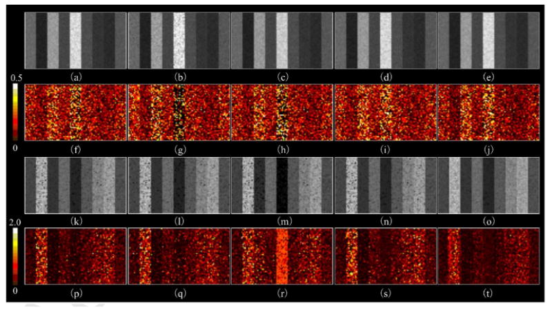
A visual presentation of the estimated ADC and AKC maps using noised synthetic DWI data (SNR = 30). (a ∼ e) are the ADC maps calculated by UNLS, CLLS, CML, CAIS, and SCAIS, and, (f ∼ j) are their corresponding residual maps (absoluate difference between the resulting maps and their reference maps); (k ∼ o) are the AKC maps by UNLS, CLLS, CML, CAIS, and SCAIS, and (p ∼ t) their residual maps. The results (particularly the residual maps) showed that our SCAIS method (last column) performed more robustly to noise than other methods, and estimation error of CLLS raised significantly at regions of high ADC values (left side portion of (g)).
As to computational efficiency, we had to choose not to compare the exact time cost of each algorithm. Because calculation time strongly depend on implementations of methods, although we conducted the experiments universally on the same hardware and did find that our proposed methods CAIS/UAIS/SCAIS/SUAIS cost less than a fraction of second, while all the other methods cost in the scale of seconds (modified CLLS/ULLS/WCLLS/WULLS), minutes (CNLS/ UNLS/ UML/CML). Based on our implements, our CAIS/ UAIS and SCAIS/SUAIS actually took only around 0.3 second.
In addition, the inspection on the convergence performance showed that the estimation error of all our 3 AIS methods decreased quickly and became comparatively stable within less number of iterations (generally only 2 ∼ 3 iterations) than the UNLS method in every noise level (Fig. 5, Rows 2, 3, 4). The UAIS method needed 10 ∼ 12 iterations to converge. While iteration number decreased to 8 ∼10 when constrains were superimposed (namely CAIS method, Fig. 5 Row 3), and the number further decreased to 6 ∼ 8 when smoothing was applied (namely SCAIS, Fig. 5 Row 4).
Figure 5.
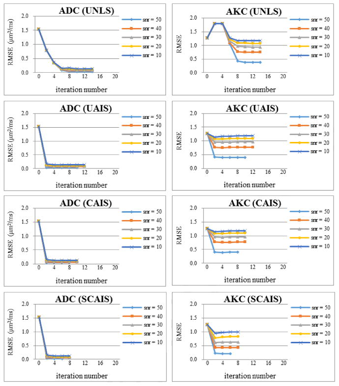
The convergence performance of the UNLS method and the three versions of AIS methods using the synthetic data. Each row displays the results of ADC and AKC calculated from one particular method (from top to bottom: UNLS, UAIS, CAIS and SCAIS, respectively). The result showed that all our AIS method converged more quickly than did the UNLS method. Note these comparisons compared purely the number of iterations without considering the huge saving of time in each iteration that our methods cost over that of the UNLS method.
The evaluation of the impact of the smoothing procedure on AKC maps showed that smoothing ADC did have direct influence on AKC estimation. The mean RMSE of AKC thus estimated were 0.3118, 0.2245, 0.1839, 0.1837, 0.1943 when FWHM was set from 0.5 to 3.0 pixels, and the lower RMSE appeared at FWHM in the range between1.5 and 2.0 pixels. The comparison of AKC residual map indicated that when FWHM ≥ 2.0 pixels, unexpected artifacts (e.g., line-structure) began to appear (Fig. 6).
Figure 6.

An evaluation of smoothing procedure in SCAIS using residual map of AKC. Five levels of Gaussian kernel FWHM were set at 0.5, 1.0, 1.5, 2.0 and 3.0 pixels. The results showed that obvious artifacts were introduced in AKC estimation by applying serious smoothing (FWHM of Gaussian kernel ≥ 2.0 pixels), while using a moderate FWHM at 1.0 ∼ 1.5 pixels may achieve well noise suppression without producing artifacts.
In general, the SCAIS method appeared to perform the best among all these opponents.
3.2.2 Synthetic Data for Bi-Exponential Model
The results using the bi-exponential model again confirmed a consistent conclusion as in Section 3.2.1 that in the case of using the bi-exponential model, our proposed methods (with and without constraints) could still perform equally or better than the other methods. The RMSE values of ADC and AKC maps calculated from most of the methods were very close to each other, and our SCAIS method achieved the lowest RMSE at every noise level (Fig. 7). Again, our CAIS/UAIS and SCAIS/SUAIS methods took only around 0.01 second, which was by far the fastest ones compared with all the other methods, based on our experiment implementation and the identical hardware.
Figure 7.
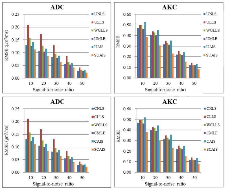
A RMSE comparison of parameter estimation methods using synthetic dataset for bi-exponential model. Estimation methods either without (upper) or with (lower) constraints was included. The RMSE of the resulting ADC (left) and AKC (right) maps showed again that our AIS methods provided similar or better results compared to other methods, and SCAIS performed the best.
In general, the experiment results using simulated datasets suggested that our proposed methods indeed can perform equally or better than the other methods that are popularly in use, but significantly faster.
3.2.3 Real data
The comparison between UNLS and UAIS showed once again that ADC and AKC maps calculated from these two methods had similar visual appearance (Fig. 8) and similar RMSE (averaged over 5 volunteers). The RMSE of ADC and AKC calculated using our UAIS method differed only slightly (difference around 0.01) from those using the conventional UNLS method in 6b, 5b and 4b cases (Table 2).
Figure 8.
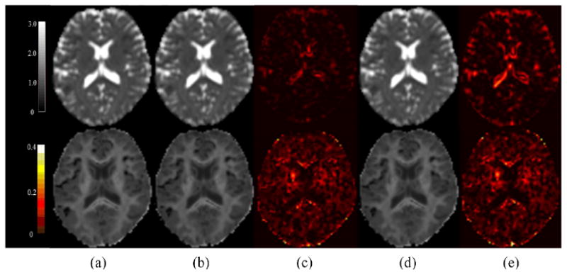
A typical example of the Mean Diffusion (MD) and Mean Kurtosis (MK) map generated by the UNLS and UAIS methods based on human data. The MD (first row) and MK (second row) maps of one volunteer were calculated from a 4b DKI dataset. (a) the reference map (using 12b DWI data, UNLS); (b) & (c) maps of UNLS method and their corresponding residual maps; (d) & (e) maps of UAIS and its residual map. The results showed that the UNLS and UAIS methods generated visually similar MD and MK maps using the 4b dataset.
The computational time of our UAIS method is less than two minutes, varying with the number of b-values involved in each combination (Table 2). It took about 116 seconds in 6b cases and 7 seconds in 3b cases.
The test of convergence speed using these real datasets showed also that our UAIS method converged quickly and became comparatively stable within less than 6 iterations (Fig. 9). The CAIS and SCAIS methods also converged very quickly within 3 to 6 iterations. As predefined in the Experiment Design Section, the iteration terminated whenever the updating differences of the estimated ADC and AKC values were below a predefined threshold.
Figure 9.
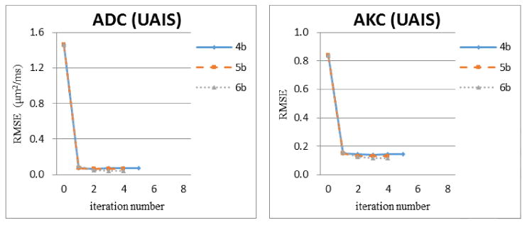
The convergence property of our UAIS method using real data. The average RMSE of resulting ADC (Left) and AKC (Right) along all gradient direction were calculated after each iteration step. The result showed again that our method converged quickly within 4∼5 iterations.
The visual comparison between our three AIS schemas showed that the constraints and smoothing procedures have significant impacts on the quality of the estimation of kurtosis maps. We observed unwanted effect of dark band in AKC and MK maps estimated using UAIS and CAIS methods as well as in the reference map where ADC was low and AKC high (Fig. 10). In contrast, AKC and MK maps of SCAIS showed no dark-band effect, and meanwhile significantly enhanced tissue visibility in the AKC map (Fig. 10), making the details of delicate structures in the brain highly visible (Fig. 11). The additional computational time for smoothing procedures was limited, taking only an extra of 20 ∼ 40 seconds in total for the datasets we used in this work, depending on the number of iterations needed to achieve sufficient accuracy.
Figure 10.
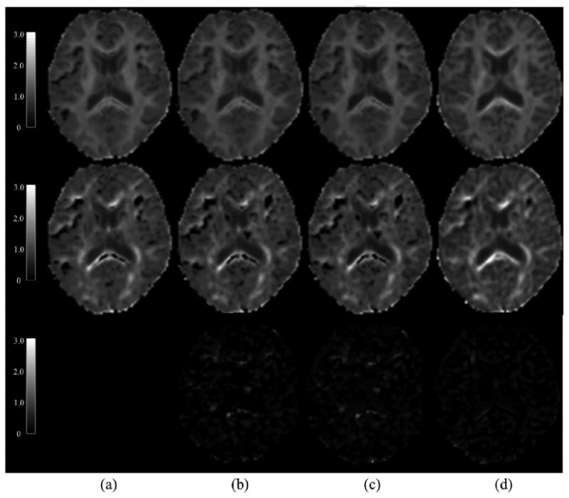
A typical example of the MK and AKC maps generated by our AIS methods. The MK map (first row) and the AKC map (second row) from one typical gradient direction were estimated from a DKI sub-dataset of 4 b-values, the difference maps of AKC (third row ) were also calculated between the reference map and the map of each individual AIS method. (a) the reference maps of MK and AKC; (b) maps calculated by UAIS method; (c) maps by CAIS; (d) maps by SCAIS. The result showed that AKC and MK maps of SCAIS had no dark band effect, and meanwhile SCAIS enhanced tissue visibility of the structural details in the AKC and MK maps. Moreover, the difference maps showed that AKC map from SCAIS was most similar to the reference maps than other two methods. Please note that the difference contains also voxels where SCAIS had more accurate estimation whereas the UNLS method generated black band.
Figure 11.

A comparison of details in MK maps. A region of interest was amplified for better visualization. (a) the reference map of MD; (b) the reference map of MK, (c) MK calculated by the UAIS method; (d) MK by CAIS; (e) MK by SCAIS. In the region of the yellow circle, we can see more structural details in the result by the SCAIS method. In the regions of yellow ellipse, the SCAIS method fixed the dark band that did not exist in the MD map, but the other methods failed.
4. Discussion
The conventional methods calculate ADC and AKC value using nonlinear curve fitting, costing huge amount of computational time to achieve adequate accuracy. We propose in this paper the AIS method family with great efficiency for DKI parameter estimation which uses an iterative schema to calculate ADC and AKC alternately. It reduces the computational time to only 1 or 2 minutes for processing one complete DKI dataset of a real-world brain. The AIS method has three versions. UAIS is the unconstrained AIS method. Our experiments have shown that UAIS can very well approximate the conventional UNLS method but with significantly accelerated speed. This high efficiency attributes to the following three factors: (1) the rapid alternative updating procedure, (2) low computational cost using linear computation in each iterative step, and consequently (3) the fast convergence nature of the solution for fast reaching stability.
In addition, by incorporating the constraints and the smoothing operation, our CAIS and SCAIS methods provide equal or even better accuracy in calculating DKI parameters; therefore, they are better alternatives readily to replace the conventional UNLS method. We have seen that our SCAIS method has provided generally the best performance (accuracy, precision, convergence). In particular, the smoothing procedure in SCAIS can significantly improve the estimation accuracy and precision of AKC. Due to these advantages, the SCAIS method can effectively suppress the dark band effect often seen in the DKI maps generated by conventional methods (Fig. 11), which are not supposed to present and therefore is actually a born defect of the UNLS method. For example, these dark bands were also surprisingly reported in the splenium and the genu of the corpus callosum from previous work when UNLS was employed [22]. Using our real data with a preprocessing step of DWI data smoothing in addition to eddy-current correction and other routine processing procedures, the SCAIS method completely removed the dark bands in MK and AKC maps. Moreover, SCAIS greatly enhances the visibility of the fine brain structures that are usually invisible in the DKI maps generated by those regular methods (Figs. 8 and 9). These desired features are extremely useful for subsequent processing steps using the DKI data, such as image segmentation or DKI-based fiber tracking.
The CLLS method was recently proposed for accelerating DKI estimation [22]. This method provided another way to degenerate the nonlinear DKI function to a linear one, which treats the 2nd order term of ADC (containing AKC) in the nonlinear function as one linear variable. Thus, DKI parameters can be calculated by a linear least squares method with very high computational efficiency. In the experiments, we have seen that the ADC estimated from CLLS method has higher estimation error (Fig. 2), which is probably due to inappropriately weighting the logarithm-transformed term in the cost function Eq. (3).
Compared to other methods, our AIS methods have two major advantages. First, different from UNLS, CML and CLLS, our method adopts a framework of alternative iteration, and uses the strong dependency between ADC and AKC values. As discussed in the Method section, a small estimation error (may originated from noise) of ADC may cause significant variation in AKC calculation. Therefore, we proposed SCAIS method to smooth ADC map in each iteration for progressively more accurate estimation of AKC in addition to applying biological and physical constraints. The experiments showed that SCAIS method has successfully improved the quality of MK map. Second, compared to the CLLS method that demands DKI data along at least 15 gradient directions, our method imposes no mandatory requirements on the number of gradient directions. It can also be incorporated easily into other reconstruction models, such as 2nd and 4th order tensor model (for AKC) or spherical harmonics model, to calculate more robust and valuable quantities.
Moreover, whereas the conventional methods adopt different strategies for treating datasets acquired with 3 b-values and datasets acquired with more than 3 b-values, our schema uses a uniform framework in which the 3 b-values dataset is only a special instance that can serve as a parameter initialization for the subsequent iterations. Therefore, our approach is relatively more flexible and can be applied to DKI datasets acquired using an arbitrary number of b-values (certainly, no less than 3) and gradient directions.
One limitation of our method is that it does not calculate the diffusion and kurtosis tensors, and consequently it will not directly provide those tensor-based quantities, such as the axial and radial coefficients of diffusion or kurtosis. Nevertheless, the proposed AIS approaches indeed provide fast and nice approximations to calculate the most frequently used measures, i.e., MD and MK, simply by averaging ADC and AKC values along all gradient directions, which may facilitate the real time applications of DKI.
The noise in MRI data is known to be Rician. Using a wrong model may introduce bias in parameter estimation. However, the noise is Rician only when the data are of SNR < 2.0, and the Rician noise will reduce to Gaussian when SNR > 2.0 [28]. Therefore, we can process the noise in DKI using a Gaussian model. In addition, this bias of noise in diffusion data can be well handled by image denoising methods [29]. In the experiment that inspected the estimation bias of each method, CML was particularly designed for treating Rician noise. The result showed that the CML method and the other methods generated very similar ADC and AKC values even at high noise levels (Fig. 7). This experiment verified that Rician bias was not an issue in our data.
As shown in the experiment that studied the ADC smoothing effect involved in SCAIS, we must use an appropriate smoothing kernel. Excessive smoothing will otherwise introduce extra artifacts into AKC estimation, for example, when FWHM of Gaussian kernel ≥ 2.0 pixels in our case. Thus, we recommend a moderate FWHM at 1.0 to 1.5 pixels or 2 to 3 mm (for real brain data) to balance between the original imaging noise level and the resulting artifacts.
Finally, DKI is a young MR diffusion modality and we expect that in the near future many research and clinical applications would take use of this new modality, as the major MR scanner manufacturers have recently begun to implant DKI in their new platforms. We also have made some efforts towards this direction in a clinical study on epilepsy, which have demonstrated satisfactory results and generated interesting findings [18].
Acknowledgments
The authors thank Jelle Veraart for providing the code of a modified version of CML method for ADC and AKC estimation. This paper is supported in part by a Grant from Shanghai Commission of Science and Technology (Grant# 10440710200), China; a Grant from the Fostering Program of a China National Nature Science Foundation Key Project (Approval # 91232701); a Grant from the 12th Five-year Plan Supporting Project of the Ministry of Science and Technology of the People's Republic of China (Grant# 2013BAI10B03); a Grant from the Large Instruments Open Foundation of East China Normal University, and in part by an NIH / NIMH Grant P50 MH090966-01, and an NIBIB Grant 1R03EB008235-01A1.
Biography
Xu Yan is a Ph.D. candidate in the Department of Physics, East China Normal University. His research interest includes post-processing and analysis methods for diffusion imaging and other MRI based techniques.
MinXiong Zhou is a Ph.D. candidate in the Department of Physics, East China Normal University. Her research interest focuses on MR image processing.
Lingfang Ying is a Master in the Department of Advanced Interdisciplinary Research, East China Normal University. Her research interest focuses on data analysis and clinical applications of diffusion imaging.
Wei Liu is a Ph.D. in the Department of Physics, East China Normal University. She studied in Psychiatry Department of Columbia University as a visiting student, during 2008–2011. Her research interest focuses on post-processing of diffusion tensor images and related analysis.
Guang Yang received his Ph.D. from Department of Physics, East China Normal University. Now he is an associate professor in Shanghai Key Laboratory of Magnetic Resonance, East China Normal University. His research interest includes MRI image processing and experiments simulation.
Dongmei Wu works in Shanghai Key Laboratory of Magnetic Resonance, East China Normal University. Her research interest includes MRI image processing and sequence development.
Yongdi Zhou obtained his Ph.D. in neuroscience from University of California, Los Angeles, now is a professor and the dean of the School of Psychology, East China Normal University. His research interest focuses on the cognitive neuroscience and neurophysiology.
Bradley S. Peterson is a Suzanne Crosby Murphy Professor of Psychiatry in the Department of Psychiatry, Columbia University. His research interest focuses on neuroimaging and brain disorders.
Dongrong Xu obtained his Ph.D. in computer science from Zhejiang University, now is an associate professor at Columbia University College of Surgeon and Surgery and a senior research scientist at New York State Psychiatric Institute. His research interest includes biomedical image processing and analysis and virtual reality technology in brain function research, and scientific visualization.
Footnotes
Publisher's Disclaimer: This is a PDF file of an unedited manuscript that has been accepted for publication. As a service to our customers we are providing this early version of the manuscript. The manuscript will undergo copyediting, typesetting, and review of the resulting proof before it is published in its final citable form. Please note that during the production process errors may be discovered which could affect the content, and all legal disclaimers that apply to the journal pertain.
Contributor Information
Xu Yan, Email: maxwell4444@hotmail.com.
Minxiong Zhou, Email: zhoumin_ecnu@163.com.
Lingfang Ying, Email: sullyying@126.com.
Wei Liu, Email: weiliu925@gmail.com.
Guang Yang, Email: gyang@phy.ecnu.edu.cn.
Dongmei Wu, Email: dmwu@phy.ecnu.edu.cn.
Yongdi Zhou, Email: yzhou12.yd@gmail.com.
Bradley S. Peterson, Email: PetersoB@nyspi.columbia.edu.
References
- 1.Basser PJ, Mattiello J, LeBihan D. MR diffusion tensor spectroscopy and imaging. Biophys J. 1994;66(1):259–267. doi: 10.1016/S0006-3495(94)80775-1. [DOI] [PMC free article] [PubMed] [Google Scholar]
- 2.Niendorf T, Dijkhuizen RM, Norris DG, van Lookeren Campagne M, Nicolay K. Biexponential diffusion attenuation in various states of brain tissue: implications for diffusion-weighted imaging. Magn Reson Med. 1996;36(6):847–857. doi: 10.1002/mrm.1910360607. [DOI] [PubMed] [Google Scholar]
- 3.Maier SE, Vajapeyam S, Mamata H, Westin CF, Jolesz FA, Mulkern RV. Biexponential diffusion tensor analysis of human brain diffusion data. Magn Reson Med. 2004;51(2):321–330. doi: 10.1002/mrm.10685. [DOI] [PubMed] [Google Scholar]
- 4.Wedeen VJ, Hagmann P, Tseng WY, Reese TG, Weisskoff RM. Mapping complex tissue architecture with diffusion spectrum magnetic resonance imaging. Magn Reson Med. 2005;54(6):1377–1386. doi: 10.1002/mrm.20642. [DOI] [PubMed] [Google Scholar]
- 5.Tuch DS. Q-ball imaging. Magn Reson Med. 2004;52(6):1358–1372. doi: 10.1002/mrm.20279. [DOI] [PubMed] [Google Scholar]
- 6.Jensen JH, Helpern JA, Ramani A, Lu H, Kaczynski K. Diffusional kurtosis imaging: the quantification of non-gaussian water diffusion by means of magnetic resonance imaging. Magn Reson Med. 2005;53(6):1432–1440. doi: 10.1002/mrm.20508. [DOI] [PubMed] [Google Scholar]
- 7.Liu C, Bammer R, Acar B, Moseley ME. Characterizing non-Gaussian diffusion by using generalized diffusion tensors. Magn Reson Med. 2004;51(5):924–937. doi: 10.1002/mrm.20071. [DOI] [PubMed] [Google Scholar]
- 8.Lu H, Jensen JH, Ramani A, Helpern JA. Three-dimensional characterization of non-gaussian water diffusion in humans using diffusion kurtosis imaging. NMR Biomed. 2006;19(2):236–247. doi: 10.1002/nbm.1020. [DOI] [PubMed] [Google Scholar]
- 9.Hui ES, Cheung MM, Qi L, Wu EX. Towards better MR characterization of neural tissues using directional diffusion kurtosis analysis. Neuroimage. 2008;42(1):122–134. doi: 10.1016/j.neuroimage.2008.04.237. [DOI] [PubMed] [Google Scholar]
- 10.Kuder TA, Stieltjes B, Bachert P, Semmler W, Laun FB. Advanced fit of the diffusion kurtosis tensor by directional weighting and regularization. Magnetic Resonance in Medicine. 2012;67(5):1401–1411. doi: 10.1002/mrm.23133. [DOI] [PubMed] [Google Scholar]
- 11.Veraart J, Van Hecke W, Sijbers J. Constrained maximum likelihood estimation of the diffusion kurtosis tensor using a Rician noise model. Magn Reson Med. 2011;66(3):678–686. doi: 10.1002/mrm.22835. [DOI] [PubMed] [Google Scholar]
- 12.Veraart J, Poot DH, Van Hecke W, Blockx I, Van der Linden A, Verhoye M, et al. More accurate estimation of diffusion tensor parameters using diffusion Kurtosis imaging. Magn Reson Med. 2011;65(1):138–145. doi: 10.1002/mrm.22603. [DOI] [PubMed] [Google Scholar]
- 13.Wu EX, Cheung MM. MR diffusion kurtosis imaging for neural tissue characterization. NMR Biomed. 2010;23(7):836–848. doi: 10.1002/nbm.1506. [DOI] [PubMed] [Google Scholar]
- 14.Jensen JH, Helpern JA. MRI quantification of non-Gaussian water diffusion by kurtosis analysis. NMR Biomed. 2010;23(7):698–710. doi: 10.1002/nbm.1518. [DOI] [PMC free article] [PubMed] [Google Scholar]
- 15.Falangola MF, Jensen JH, Babb JS, Hu C, Castellanos FX, Di Martino A, et al. Age-related non-Gaussian diffusion patterns in the prefrontal brain. J Magn Reson Imaging. 2008;28(6):1345–1350. doi: 10.1002/jmri.21604. [DOI] [PMC free article] [PubMed] [Google Scholar]
- 16.Helpern JA, Adisetiyo V, Falangola MF, Hu C, Di Martino A, Williams K, et al. Preliminary evidence of altered gray and white matter microstructural development in the frontal lobe of adolescents with attention-deficit hyperactivity disorder: a diffusional kurtosis imaging study. J Magn Reson Imaging. 2011;33(1):17–23. doi: 10.1002/jmri.22397. [DOI] [PMC free article] [PubMed] [Google Scholar]
- 17.Raab P, Hattingen E, Franz K, Zanella FE, Lanfermann H. Cerebral gliomas: diffusional kurtosis imaging analysis of microstructural differences. Radiology. 2010;254(3):876–881. doi: 10.1148/radiol.09090819. [DOI] [PubMed] [Google Scholar]
- 18.Yuzhen Zhang XY, Gao Yu, Xu Dongrong, Wu Jie, Li Yuhua. A Preliminary Study of Epilepsy in Children Using Diffusional Kurtosis Imaging. Clinical Neuroradiology. 2013;23(4):293–300. doi: 10.1007/s00062-013-0212-3. [DOI] [PubMed] [Google Scholar]
- 19.Jansen JF, Stambuk HE, Koutcher JA, Shukla-Dave A. Non-gaussian analysis of diffusion-weighted MR imaging in head and neck squamous cell carcinoma: A feasibility study. AJNR Am J Neuroradiol. 2010;31(4):741–748. doi: 10.3174/ajnr.A1919. [DOI] [PMC free article] [PubMed] [Google Scholar]
- 20.Cheung MM, Hui ES, Chan KC, Helpern JA, Qi L, Wu EX. Does diffusion kurtosis imaging lead to better neural tissue characterization? A rodent brain maturation study Neuroimage. 2009;45(2):386–392. doi: 10.1016/j.neuroimage.2008.12.018. [DOI] [PubMed] [Google Scholar]
- 21.Jensen JH, Hu C, Helpern JA. Rapid Data Acquisition and Post-processing for Diffusional Kurtosis Imaging. 2009:1403. [Google Scholar]
- 22.Tabesh A, Jensen JH, Ardekani BA, Helpern JA. Estimation of tensors and tensor-derived measures in diffusional kurtosis imaging. Magn Reson Med. 2011;65(3):823–836. doi: 10.1002/mrm.22655. [DOI] [PMC free article] [PubMed] [Google Scholar]
- 23.Madsen K, N HB, Tingleff O. Methods for Non-Linear Least Squares Problems. 2nd. IMM; 2004. [Google Scholar]
- 24.Salvador R, Pena A, Menon DK, Carpenter TA, Pickard JD, Bullmore ET. Formal characterization and extension of the linearized diffusion tensor model. Hum Brain Mapp. 2005;24(2):144–155. doi: 10.1002/hbm.20076. [DOI] [PMC free article] [PubMed] [Google Scholar]
- 25.Bjõrck A. Numerical Methods for Least Squares Problems. SIAM; 1996. [Google Scholar]
- 26.Tabesh A, Jensen JH, Ardekani BA, Helpern JA. Estimation of tensors and tensor-derived measures in diffusional kurtosis imaging. Magn Reson Med. 2011 doi: 10.1002/mrm.22655. [DOI] [PMC free article] [PubMed] [Google Scholar]
- 27.Xu Yan MZ, Lingfang Ying, Dazhi Yin, Mingxia Fan, Guang Yang, Yongdi Zhou, Fan Song, Dongrong Xu. Evaluation of Optimized b-Value Sampling Schemas for Diffusion Kurtosis Imaging with an Application to Stroke Patient Data. Computerized Medical Imaging and Graphics. 2013 doi: 10.1016/j.compmedimag.2013.04.007. In Press. [DOI] [PMC free article] [PubMed] [Google Scholar]
- 28.Gudbjartsson H, Patz S. The Rician distribution of noisy MRI data. Magn Reson Med. 1995;34(6):910–914. doi: 10.1002/mrm.1910340618. [DOI] [PMC free article] [PubMed] [Google Scholar]
- 29.Descoteaux M, Wiest-Daessle N, Prima S, Barillot C, Deriche R. Impact of Rician adapted Non-Local Means filtering on HARDI. Int Conf Med Image Comput Comput Assist Interv (MICCAI) 2008;11(2):122–130. doi: 10.1007/978-3-540-85990-1_15. [DOI] [PubMed] [Google Scholar]


