Not Just the Norm: Exemplar-Based Models also Predict Face Aftereffects

Abstract

The face recognition literature has considered two competing accounts of how faces are represented within the visual system: Exemplar-based models assume that faces are represented via their similarity to exemplars of previously experienced faces, while norm-based models assume that faces are represented with respect to their deviation from an average face, or norm. Face identity aftereffects have been taken as compelling evidence in favor of a norm-based account over an exemplar-based account. After a relatively brief period of adaptation to an adaptor face, the perceived identity of a test face is shifted towards a face with opposite attributes to the adaptor, suggesting an explicit psychological representation of the norm. Surprisingly, despite near universal recognition that face identity aftereffects imply norm-based coding, there have been no published attempts to simulate the predictions of norm- and exemplar-based models in face adaptation paradigms. Here we implemented and tested variations of norm and exemplar models. Contrary to common claims, our simulations revealed that both an exemplar-based model and a version of a two-pool norm-based model, but not a traditional norm-based model, predict face identity aftereffects following face adaptation.

Introduction

Faces, unlike many common objects, are recognized individually, placing particular demands on the visual system to rapidly and accurately distinguish between large numbers of visually similar patterns. The face-space framework (Valentine, 1991) has offered a useful starting point for understanding how the visual system might solve this recognition problem. Building on other successful models of visual cognition (e.g., see Ashby, 1992), face space assumes that faces are represented within a multidimensional psychological space. Specific theories differ with respect to how faces are represented in that space, including whether they are represented as norms or exemplars. Norm-based accounts propose that faces are encoded with respect to their deviation from the average face, or norm¹ (e.g., Giese & Leopold, 2005; Rhodes & Jeffery, 2006; Valentine, 1991). Exemplar-based accounts propose that faces are encoded by their location in face space relative to exemplars of previously experienced faces (e.g., Lewis, 2004; Valentine, 1991).

Both norm- and exemplar-based theories account for many key phenomena associated with face recognition, such as the effects of distinctiveness, race, and caricature on recognition and categorization (e.g., see Valentine, 1991). Differentiating between norm- and exemplar-based models has proved to be a substantial challenge. To illustrate, let us first consider briefly how recognition of face caricatures has impacted the norm versus exemplar debate. Interest in caricatures comes from the observation that, especially when well done, artist-drawn caricatures often seem to be “super portraits” (Rhodes, 1996), somehow capturing the identity of the person being caricatured better than a faithful portrait or photograph. Indeed, in more controlled laboratory settings it has been shown that caricatures are often recognized more quickly and more accurately than the veridical images from which they were created (e.g. Benson & Perrett, 1994; Lee & Perrett, 1997; Rhodes, Brennan, & Carey 1987; Rhodes & Tremewan, 1994, but see Hancock & Little, 2011). Because caricature exaggerates a face's deviation away from the average, it is commonly assumed that norm-based models provide a natural account of the caricature effect. Perhaps less appreciated is that exemplar-based models can also predict the caricature effect (e.g., Lewis, 2004; Lewis & Johnston, 1998, 1999). For example, in Lewis’ (2004) Face-space-R model, the caricature effect emerges as a result of the exemplar density gradient between the center of the face space and its outer reaches. While a faithful photograph of a given face may be closer to the target exemplar than a caricature of the same face, it may also be closer to other, irrelevant, exemplars. As a result, slightly caricatured face will often activate the corresponding exemplar-representation proportionally more strongly than the veridical image.

More recently, research into face aftereffects has offered new insights into the nature of the representations underlying face recognition. Face aftereffects, much like their low level counterparts such as motion or tilt aftereffects (Gibson & Radner, 1937; Mather, Verstraten & Anstis, 1998), are short-lived perceptual biases induced by brief exposure to an adapting stimulus. Just as briefly viewing an upwards-moving pattern creates an aftereffect whereby a stationary pattern is perceived to move downwards, it seems that exposure to a distinctive face can bias our perception of what is an average face (e.g., Webster & MacLin, 1999). Several studies have demonstrated that face adaptation can induce identity-specific changes to face recognition, opening up the possibility that aftereffects might reveal how faces are represented (e.g., Jiang, Blanz, & O'Toole, 2009; Leopold, O'Toole, Vetter, & Blanz, 2001; Rhodes & Jeffery, 2006).

In one such study, Leopold et al. (2001) used a set of carefully constructed face stimuli to differentiate between norm- and exemplar-based face-space models. To do this they first had participants learn to identify four target faces (Adam, Jim, John, or Henry). As shown in Figure 1a, the target faces can be imagined to exist within a schematic face space, with an average face occupying the center of the space, and the target faces around the periphery (only two of the four target faces are shown). Morph trajectories² were constructed from each of the four target faces, passing through the center (average) of face space, so that lying on the opposite side of the average were four “anti-faces”; for example, as shown in Figure 1a, Adam's face is longer and thinner than the average face; as a result, “anti-Adam” has a face that is shorter and fatter than average.

Figure 1.

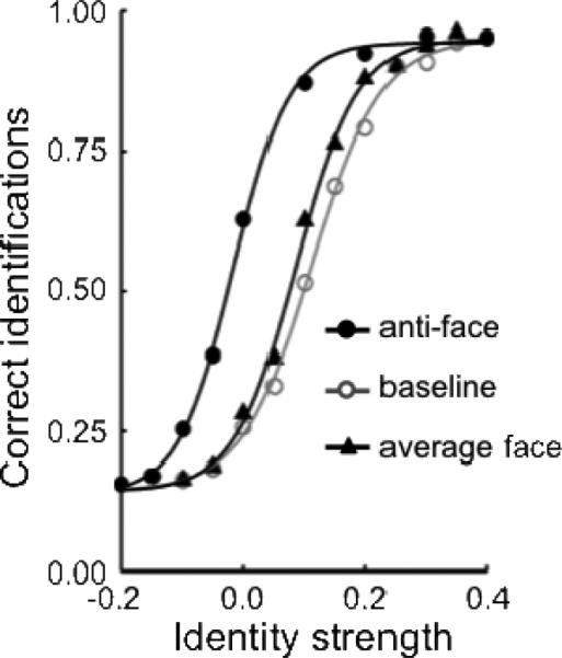
(a) Schematic face-space representation of the relationship between the stimuli used in the anti-face identity adaptation paradigm (adapted from Leopold et al., 2001). For each the four target faces (only two shown here) an anti-face adaptor was constructed so as to lie on the opposite side of the average face (John vs. anti-John, Adam vs. anti-Adam). (b) Sensitivity to face identity with (matching and non-matching) and without (baseline) adaptation (data points from Leopold et al, 2001). Three conditions are shown: baseline identity accuracy without any adaptation (○), identity accuracy following adaptation to a matching anti-face (●) (e.g., adapting to anti-Adam, then testing with Adam), identity accuracy following adaptation to a non-matching anti-face (■) (e.g., adapting to anti-John, then testing with Adam). The proportion of correct responses at each identity level has been averaged across the four identity trajectories and a best-fitting four parameter logistic function is shown for each condition (following Leopold et al., 2001).

On each trial of the face identity task, participants were presented with a test face selected from some location along one of the four morph trajectories, ranging from 1.0 for a target face, 0.5 for a face halfway between the target and the average, 0.0 for the average face, with negative proportions for anti-faces on the opposite side of the average. The participant's task was simply to identify the test face as Adam, Jim, John, or Henry. Because all four trajectories passed through the average, participants could only guess which of the four morph-trajectories the average face belonged to. This is illustrated in the baseline psychometric function in Figure 1b (from Leopold et al., 2001), which plots face identification accuracy as a function of the location of a face along its morph trajectory.

On some trials, participants were first briefly adapted for a few seconds to one of the anti-faces before being shown the test face. On baseline trials, a blank screen preceded the test face. As illustrated in Figure 1b, relative to baseline, adaptation to a matching anti-face, for example, adapting to anti-Adam when the test face was from the Adam morph-trajectory, biased perception of a test face towards the target face that the anti-face was generated from. That is to say, participants were better at identifying the target identity after adapting to its anti-face. This is reflected by the shift in the psychometric function to the left following adaptation to the matching anti-face. In addition, when the adapting anti-face was non-matching, for example, if the test face was selected from the Henry morph-trajectory but the anti-face was anti-Jim, the psychometric function was shifted to the right, indicating that adaptation actually impaired target face identification. So the direction of the aftereffects was quite specific, with opposite anti-face adaptors enhancing target face identification but non-matching anti-face adaptors hindering it.

Leopold et al. (2001) took these findings to suggest that adaptation biases perception towards a face that lies on the opposite side of the average to the adaptor. In other words, just as upward motion seems to be represented by the visual system as the opposite of downward motion, there appears to be a real psychological sense in which the anti-faces in Leopold et al. (2001) were opposite each of their respective target faces. From the perspective of the norm versus exemplar debate, these findings have been considered important because they suggest that the visual system must have an explicit means of representing the relationship between a given face and the average face. Exemplar-based models have no explicit sense in which the anti-faces lie opposite to the target faces, since faces are simply locations in face space. In contrast, norm-based models explicitly represent faces with respect to the norm, or average face, making each anti-face psychologically opposite to its corresponding target face. From this, Leopold et al. (2001) concluded that face identity aftereffects provided evidence for “prototype-referenced” or norm-based shape encoding of faces.

There has been substantial empirical work aimed at understanding face identity adaptation and its relation to the norm-versus-exemplar debate since Leopold et al.'s (2001) demonstration. These findings and several subsequent extensions of the anti-face paradigm (e.g., Jeffery et al., 2010; Leopold & Bondar, 2005; Rhodes & Jeffery, 2006) have lead to a widespread acceptance of the norm-based account of face representation (e.g., Griffin, McOwan, & Johnston, 2011; Jeffery et al., 2010; Leopold & Bondar, 2005; Leopold et al., 2001; Nishimura et al. 2010; Nishimura et al., 2008; Nishimura, Robertson, & Maurer, 2011; Palermo et al, 2011; Pellicano et al., 2007; Rhodes & Jaquet, 2011; Rhodes, et al., 2011; Rhodes & Jeffery, 2006; Rhodes & Leopold, 2011; Rhodes et al., 2005; Rhodes et al., 2010; Robbins, McKone, & Edwards, 2007; Short, Hatry, & Mondloch, 2011; Susilo, McKone, & Edwards, 2010a; Susilo, McKone, & Edwards, 2010b; Tsao & Freiwald, 2006).

However, despite the apparent convergence on a norm-based account, to date there has been little attempt to generate formal predictions about face identity aftereffects using mathematical or computational instantiations of norm- or exemplar-based models. Sometimes, predictions are generated from intuitions or illustrations of idealized one- or two-dimensional face spaces. But intuitions can be misleading. This is particularly true when the models include features such as high-dimensionality, non-linear activation functions, learning mechanisms, and the like (e.g., see Burton & Vokey, 1998; Hintzman, 1990; Lewis, 2004; Palmeri & Cottrell, 2010). To address this omission, we implemented simple versions of norm- and exemplar-based models and tested their predictions regarding face identity aftereffects. Contrary to common suggestions, our simulations revealed that both an exemplar-based model and a version of a two-pool norm-based model, but not a traditional norm-based model, predicted face identity aftereffects following face adaptation.

Computational Modeling Methods

In this section we describe three different implementations of the face-space model. Following the work of Valentine (1991), we instantiated an exemplar-based model, which bore similarities to exemplar models of categorization (e.g., Kruschke, 1992; Nosofsky, 1986). In addition, we instantiated two versions of the norm-based model; a traditional norm-based model, based on a norm-based model formalized by Giese and Leopold (2005), and a two-pool norm-based model, adapted from theoretical descriptions of norm-based coding in the face recognition literature (e.g., Rhodes & Jeffery, 2006). We attempted to keep these instantiations in line with previous descriptions in the face recognition literature while also relating them to computational models in the categorization literature. Note that some of the decisions that we made regarding implementation are further addressed in the General Discussion section.

The basics of the common model architectures are illustrated in Figure 2. To enable direct comparisons between the three models, we assumed the exact same perceptual input representation and output decision mechanism for every model. All that varied across the three was the internal face-space representation (Face-Space Layer in Figure 2a). To outline, when a test face, for example Adam, is presented for identification, a multidimensional perceptual representation is created by the visual system (f). The multidimensional representation of the test face activates exemplars, norms, or pools in the face-space layer (k_i) according to the rules for that particular model of face space. The distributed pattern of activity across these exemplars, norms, or pools is associated via connection weights (w) with identity nodes for Adam, Jim, John, or Henry (o_j). Connection weights were learned using a standard delta-rule learning algorithm as an early step in the simulations. Identification probabilities are calculated as a function of the activation of the identity nodes (following, e.g., Kruschke, 1992). Finally, as detailed later, a common set of simple assumptions was made in order to implement adaptation within the three models.

Figure 2.

Illustration of the model architectures. (a) Schematic representation of the activation functions in the three models. Left: Face representations in the exemplar-based model (e.g., Lewis, 2004). Middle: Face representations in the traditional norm-based model (e.g., Giese & Leopold, 2005). Right: Face representations in the two-pool norm-based model (e.g., Rhodes & Jeffery, 2006). (b) The common architecture of the three models, assuming the same perceptual representation along the input layer and the same decisional mechanism along the output layer with structurally similar learned mappings with the intermediate face-space layer, which is the only thing that differed between the three models.

The Perceptual Representation Layer

The layer of input nodes, the perceptual representation layer, encodes the location of a presented test face along each of the perceptual dimensions, with each node encoding a particular dimension; this input layer can be thought of as the output of mid-level visual processing. The activation pattern across the full set of nodes is an -dimensional face-space vector representation, denoted in Figure 2b by the column vector f = (f₁ , f₂ , . . . f_n)^T. We implemented two versions of the perceptual representation layer for each face-space model. A Gaussian version simply assumes that a randomly sampled face is perceptually represented as a random sample from a multidimensional Gaussian distribution. A PCA-based version explicitly constructs a perceptual representation of a face image using a simple model of a perceptual front end.

Gaussian Versions

In line with some previous computational instantiations of face space (e.g., Lewis, 2004), the Gaussian versions of the three face-space models assumed that, at least for a relatively homogeneous population of faces, such as those of the same race and gender, faces are normally distributed along each of the face-space dimensions (e.g., see Valentine, 1991; also see Burton, Bruce, & Dench, 1994). Thus, the perceptual representation of a randomly sampled face is generated by randomly sampling a multidimensional vector from a multivariate Gaussian (normal) distribution. Here we make no specific assumptions about how that perceptual representation is created, just that it is. Any time a face is randomly selected, which could be when selecting faces to populate a particular simulated subject's face space, or when selecting a target face for a simulated face adaptation experiment, a new random sample is drawn from a multivariate Gaussian distribution.

Principal Component Analysis Based Versions

Whereas the Gaussian versions do not assume anything about how the multidimensional representation of a given face might be created, the PCA-based versions take actual face images as input and create a multidimensional face representation from them. Unlike some other successful visual recognition models, which assume multiple layers of visual processing (e.g., Jiang et al., 2006; Serre, Oliva, & Poggio, 2007), the PCA-based front end is computationally simple. Furthermore, PCA-based models have been successfully used in the past to explain various aspects of face recognition (e.g., Burton, Bruce, & Hancock, 1999; Dailey & Cottrell, 1999; Giese & Leopold, 2005; O'Toole, Deffenbacher, Valentin, & Abdi, 1993; Richler, Mack, Gauthier, & Palmeri, 2007). Here, rather than operate directly on the pixel intensity values of each image, we used a shape-based PCA, which operated on a set of hand-placed fiducial markers, adapted from Burton et al. (1999). This provides a natural correspondence between the morphing procedure used to create stimuli in the anti-face paradigm and the approach to creating PCA representation of the faces (see Appendix A for more information on the PCA procedure).

The Face-Space Layer

The second layer of nodes in each model, the face-space layer, instantiates competing hypotheses regarding representations in face space. This layer encodes the locations of the faces comprising the face space that is assumed to exist in the mind of the observer prior to the start of any experiment. The location of the th face representation in face space is denoted by the column vector k_j = (k_j1, k_j2, . . . k_jn)^T. Each k_j has the same dimensionality as the perceptual representation layer. The composition, representation, and activation of all k_j faces in the face-space layer depend on the rules for the particular face-space model being implemented.

In all models, we assume that face space is populated with a random sample of faces prior to any simulated experiment. In the Gaussian version of each model, each face in face space is a true random sample from a multivariate normal distribution. For the reported simulations, we assumed 500 randomly experienced faces within the face-space layer (simulations with as few as 50 faces and as many as 2000 faces in face space produced qualitatively similar predictions). In the PCA-based version of each model, the faces are selected at random from a face database with their multidimensional representation determined by the PCA. For the reported simulations, we assumed 50 randomly experienced faces within the face-space layer; a smaller number of faces was used in the PCA versions because of the limited number of faces in our face image database and because of the significant time needed to place fiducial marks on each face image.

Recall that in experiments on the face identify aftereffect, participants learn the identities of new faces (Adam, Jim, John, or Henry) at the start of the experiment. For the reported simulations, we assumed that representations of new faces learned in an experiment had a distributed representation across previously experienced faces in face space (e.g., see Edelman, 1999; Palmeri, Wong, & Gauthier, 2004) – a new face-space representation was not added for every new face learned (versions where we allowed a new face-space representation for every newly learned faces produced qualitatively similar results).

Each k_j face representation is activated according to the rules for the particular face-space model being implemented. In the exemplar-based model, each face-space representation is activated by its similarity to the presented face. In the traditional norm-based model, each face-space representation is activated depending on the angular difference and relative distance with respect to the norm of the face space. In the two-pool norm-based model, the representations are activated as competing pools on opposite sides of the norm. The distributed representation of activation across face space is associated with the identities (Adam, Jim, John, or Henry) in the output layer via learned connection weights, as described later.

Exemplar-Based Model

Following previous instantiations of an exemplar-based face-space model (e.g., Giese & Leopold, 2005; Lewis, 2004), each exemplar is represented as a location in a multi-dimensional face space. The activation of a given exemplar depends on its similarity to a test face, such that the activation (act) of a given exemplar k_j by a test face f is a nonlinear function of its distance from the test face, given by

$$ac{t}_{{\mathbf{k}}_{\mathbf{j}}\mid \mathbf{f}}=\exp \left(-\frac{{\Vert {\mathbf{k}}_j-\mathbf{f}\Vert }^2}{2{\eta }^2}\right),$$ (1)

where ∥k_j − f∥ denotes the distance between exemplar k_j and test face f. Exemplars that are closest to the test face will be activated more strongly than exemplars that are further away. The parameter η controls the similarity gradient, or broadness of tuning, of each exemplar, such that larger values of η result in the exemplar representation being less selective.³

Traditional Norm-Based Model

We refer to this instantiation of a norm-based model (Giese & Leopold, 2005) as a “traditional” norm-based model because it captures well the way norm-based models are often described in some face recognition publications, especially early ones (e.g., Loffler, Yourganov, Wilkinson, & Wilson, 2005; Rhodes, 1996; Rhodes, Carey, Byatt, & Proffitt, 1998; Valentine, 1991). These descriptions suggest that faces are represented by their direction of deviation from a norm, representing what is unique about each known identity relative to the average face. The location of the norm is defined by the central tendency of the population of faces making up the face space. In this version of a norm-based model, the activation of a given face representation is a function of the vector angle relative to an explicit norm m between the face representation in face space and the test face representation along the perceptual representation layer. Similarity between two faces is a function of the difference in their direction of deviation from the norm. Two faces that lie at different points along a particular trajectory away from the norm, such as a caricature and its veridical version, will be represented as different strength of the same identity. To formalize this, following Giese and Leopold (2005), information about the distance of a given face-space representation from the norm is not assumed to be encoded, so face-space representations in the traditional norm-based model are denoted by a unit vector k̂_j,m. The distance of a test face from the norm scales the activation, such that more distinctive test faces result in greater overall activation, although simply making a face more distinctive will not change the pattern of activation across exemplars. The activation (act) of a face representation k_j in face space given test face f is given by (Giese & Leopold, 2005)

$$ac{t}_{{\mathbf{k}}_{\mathbf{j}}\mid \mathbf{f}}=\Vert \mathbf{f}-\mathbf{m}\Vert {\left(\frac{{(\mathbf{f}-\mathbf{m})}^T{\widehat{\mathbf{k}}}_{\mathbf{j},\mathbf{m}}}{2\Vert \mathbf{f}-\mathbf{m}\Vert }+\frac{1}{2}\right)}^v,$$ (2)

where the parameter ν, which must be greater than 0, controls the broadness of tuning. The right portion of the equation within the large outer parentheses determines the difference in angular deviation between a test face f and a given face-space representation k_j with respect to the norm m. Considering only this portion of the equation, activation act_kj |f will be 0 in response to an opposite test face and 1 in response to a test face that deviates from the norm in the same direction. In the left portion of the equation, the distance of the test face from the norm, ∥f − m∥, scales the activation. If an average face were presented as a test face then all of the activations in face space would be equal to 0.

Two-Pool Norm-Based Model

A simple version of a two-pool model was implemented based on descriptions of such a theory in the literature (e.g., Rhodes & Jeffery, 2006). Without an explicit mathematical formalization to draw upon, there could be several potential ways to implement a two-pool model. As the name implies, a basic idea of a two-pool model is that nodes (pools) on either side of the norm compete with one another. Unlike the traditional norm-based model, where the norm is an explicit representation determining the activation of face nodes, in the two-pool model, the norm is implicit. When constructing the face space, every node (or pool) has an opposing node (or pool) on the other side of the norm.

Our two-pool model was formalized by creating for each face representation in face space, a second opposing face representation, which lay directly opposite to it with respect to the norm. We also assumed that the activation of each opponent pair was normalized, such that the overall activation of a pair would always equal 1. In this way, the relative activation of the two nodes in the pool depends on the position of a test face relative to a face representation's preferred direction of deviation from the norm; in this way, an average face would activate all competing pools equally. While it is not necessary in all written accounts of a two-pool model for each face representation to have a directly opposing face-representation (e.g., see Rhodes et al., 2005), this is one possible formalization of the model, and was the one we chose for our simulations. The normalized activation (act) of face representation k_j given test face f is given by

$$ac{t}_{{\mathbf{k}}_{\mathbf{j}}\mid \mathbf{f}}=\frac{ac{t}_{{\mathbf{k}}_{\mathbf{j}}\mid \mathbf{f}}^{\prime }}{ac{t}_{{\mathbf{k}}_{\mathbf{j}}\mid \mathbf{f}}^{\prime }+ac{t}_{\mathbf{opp}\mid \mathbf{f}}^{\prime }}$$ (3)

where $ac{t}_{{\mathbf{k}}_{\mathbf{j}}\mid \mathbf{f}}^{\prime }$ is the activation of the face node prior to normalization and $ac{t}_{\mathbf{opp}\mid \mathbf{f}}^{\prime }$is the activation of its competing nodes on the opposite side of face space. We assumed that act’ is given by Equation 1.

The Output Layer

The output layer has a node corresponding to each possible response r in a given task. In the face identity aftereffect experiments, this means an output node corresponding to each of the four learned face identities (Adam, Jim, John, and Henry). The activation of output node r given test face f is given by

$$ou{t}_{r\mid \mathbf{f}}=\sum _j{w}_{jr}ac{t}_{{\mathbf{k}}_{\mathbf{j}}\mid \mathbf{f}}.$$ (4)

The learned association weight between the th face-space representation and the rth response node is denoted by w_jr. Weights in a linear neural network were trained using a standard delta rule (Widrow & Hoff, 1960), with teacher signals of 1.0 for the correct face name and -1.0 for the incorrect face name. Learning continued until an error of 0.01 or 1000 epochs was reached, whichever came first.

To relate output activations of the model to human performance on a given task, the activations of the output nodes were mapped onto response probabilities using a modified version of Luce's choice rule (Luce, 1963) that has been used in previous neural network models (e.g., Kruschke, 1992). The probability of naming test face f as target face R is given by

$$P(R\mid \mathbf{f})=\frac{\exp \left(\varphi ou{t}_{R\mid \mathbf{f}}\right)}{\sum _r\exp (\varphi ,ou{t}_{r\mid \mathbf{f}})}$$ (5)

where the parameter ϕ controls how probabilistic or deterministic the probability mapping function is allowed to be. So, the probability of making a particular response, say Adam, is given by taking the exponentiated evidence for the face being Adam and dividing it by the sum of the exponentiated evidence for it being any of the possible identities.

Simulating Face Adaptation

We chose not to explicitly model details of how and why adaptation might occur within the face-space layer (Grill-Spector, Henson, & Martin, 2006; Zhao, Series, Hancock, & Bednar, 2011), but chose simply to model the consequences of adaptation as a reduced activity of face nodes in face-space layer (see Figure 3). This assumption appears consistent with some verbal descriptions of face adaptation (e.g., Rhodes & Jeffery, 2006; Rhodes & Leopold, 2012; Robins et al., 2007; Susilo, et al. 2010b; Tsao & Freiwald, 2006). Using these descriptions as a guide, we assumed that brief adaptation would temporarily reduce the maximum possible activation of each face node in proportion to its degree of activation to the adapting face.

Figure 3.

Illustration of hypothesized adaptation effects from a two-pool model (left) and exemplar-based coding model (right) reproduced from Susilo et al. (2010b). As reproduced here, the specific dimension used in their illustration is eye height. As in our version of the two-pool model, opposing pools of representations, centered on the norm, represent eye-height (i.e. the combined activity of all pools that are responsive to variations along this dimension), whereas in the exemplar-based model, eye-height is encoded by multiple representations with bell-shaped tunings. In both cases, adaptation is assumed to result in a decrease in activation of each representation in proportion to its activation by the adapting stimulus.

For the exemplar-based model and two-pool model, the post-adaptation activation of a face node (act*) to a given test face f was assumed to be scaled by an adaptation factor, such that

$$ac{t}_{k\mid f}^{\ast }=ac{t}_{k\mid f}(1-\alpha \cdot ac{t}_{k\mid adapter})$$ (6)

If α=0, no adaptation at all occurs. For 0<α<1, the post-adaptation activation of a face node is reduced in proportion to its activation by the recent adaptor (act_k|adaptor), to a degree scaled by the parameter α. Note that by Equation 1, the maximum activation (act) for these two models is 1.

Adaptation in the traditional norm-based model was implemented in an analogous way. However, because activation of a face node is not constrained between 0 and 1, we assumed that the inhibition was inversely proportional to an exponential of the activation of the face node during adaptation.

$$ac{t}_{k\mid f}^{\ast }=ac{t}_{k\mid f}\lfloor 1-\alpha \cdot \exp (-\theta ac{t}_{k\mid adapter})\rfloor ,$$ (7)

where the parameter α controls the degree of adaptation and the parameter θ controls the sharpness of the adaptation function.

Model Simulation Approach

In this article, we were interested in qualitative model predictions, not just quantitative model fits. A common approach to model testing is to find values of free parameters that optimize the fit of a model to some observed data (e.g., see Lewandowsky & Farrell, 2010). While a powerful and widely used approach to model testing – one we have used in much of our own work (e.g., Mack & Palmeri, 2010; Purcell, Schall, Logan, & Palmeri, 2012) – we were interested in testing whether each of the models could predict the observed pattern of face identity aftereffects across a wide range of parameters. While certain criticisms of quantitative model testing overgeneralize (e.g., Roberts & Pashler, 2000), it is true that some approaches to fitting models to data do not discriminate between a model that predicts a result “parameter free” from a model that could fit any possible pattern of results.

Some key parameters of each model are the number of dimensions in the perceptual and face-space representation (n), the broadness of tuning of face-space nodes (η or ν), and the strength of adaptation (α). We used a grid search to systematically explore the effects of these parameters on model predictions, whereby each of these parameters was adjusted in increments over a range of values. Other parameters (e.g., ϕ or θ) were adjusted to produce a reasonable correspondence between model predictions and previously published data (see Table 1 for parameter ranges). We do display “representative” model predictions that demonstrate good quantitative fits to published data, but because of our grid search approach, these are certainly not the best fit we could have achieved using a more rigorous parameter optimization algorithm. For the Gaussian versions, we also display “qualitative maps” across a grid of parameters values, which are color-coded according to whether the model predicts the correct qualitative pattern of results. Details of this will be described later.

Table 1.

Range of parameter values used to generate maps of qualitative predictions, defined by Lower bound, Upper bound, and Step Size (n = number of dimensions of the face space; η, ν = broadness of tuning, α = adaptation strength, ϕ = response mapping parameter, θ = adaptation scaling parameter for traditional norm-based model)..

Parameter	Lower	Upper	Step Size
n	2	50	3
η	0.6	12	0.3
ν	0.6	12	0.3
α	0.2	0.8	0.2
ϕ	2	30	2
θ	0.5	1.5	0.1

Each of the six different model variations, the three different face spaces (exemplar, traditional norm-based, or two-pool norm-based) factorially combined with two different perceptual representation layers (Gaussian or PCA), were tested on each of the implemented face identity aftereffect paradigms. Models were implemented in Matlab (using both neural network and statistical toolboxes) and simulated on a high performance computing cluster at Vanderbilt University (ACCRE). When simulating each adaptation paradigm, for each parameter set within the grid search, for each model variant, 100 simulations were conducted, randomly generating a face space and set of test faces each time. Because of the limited number of faces in our stimulus set and because the simulations were slow to execute, the PCA versions of the model were only simulated once on each paradigm using the same parameters used to generate the representative fits for the Gaussian versions. Qualitative maps were not generated for the PCA-based models because these would have taken many months of computational time to create.

Computational Modeling Results

Anti-Face Adaptation

We first applied versions of the three face-space models to the “anti-face” adaptation paradigm used by Leopold et al. (2001). As described earlier, Leopold et al. constructed morph-trajectories extending from four target faces through an average face to a set of matching anti-faces on the opposite side of the average. The primary goal of the study was to test whether adaptation to one of the anti-faces, say, anti-Adam, would facilitate recognition of the target face, Adam, on the opposite side of the average. Identification with and without adaptation to the anti-face was tested along a morph trajectory of faces extending along a line from the anti-face to the target face. Following Leopold et al., positions along that morph trajectory are referred to as identity strength, with positive values closer to the target face, negative values closer to the anti-face, and zero at the center of the space (average face). As shown in Figure 1b, Leopold et al. (2001) found that adaptation to a matching anti-face did indeed facilitate target identification, as reflected by the leftward shift of the psychometric function. By contrast, adaptation to a non-matching anti-face (e.g., adapting to anti-Jim but testing along the Adam morph trajectory) actually impaired identification somewhat.

Our simulations attempted to recreate the approach that would be used in a published behavioral experiment. We started with a set of 20 potential target faces. For the Gaussian versions of the models, these were simply 20 randomly sampled points from a multivariate normal distribution (with dimensionality determined by parameter n for that simulation). For the PCA version, these were a random sample of 20 faces from our face image database (faces that had not been used to generate the PCA). From the initial set of 20 faces, we chose four that were highly dissimilar to one another. For the Gaussian versions, these were four that were relatively far from one another in multidimensional space. For the PCA versions, these were four that had quite dissimilar PCA representations. Those were the four target faces, corresponding to Adam, Jim, John, and Henry. For every set of parameter values in the Gaussian version, we replicated this procedure 100 times to ensure that the predictions were not sensitive to the particular sample of four faces used for the simulations, so that each simulation run had a different “Adam”, “Jim”, “John”, and “Henry”.

The four morph-trajectories (extending from each of the target faces) consisted of 13 identity levels created in steps of 0.05 between the 0.40 identity level (40% of the distance from the target face to the average face) and the -0.20 identity level (a moderate anti-face, 20% on the other side of the norm from the target face). For the Gaussian versions, a simulated morph-trajectory was simply a line in face space through the average to the opposite side of face space. For the PCA versions, we morphed face images to create a morph-trajectory from each target face, through the average face, to its anti-face, exactly as we would if replicating a behavioral experiment. In the PCA model, the average face was generated from a separate set of 30 faces from the stimulus set (faces that had not used as targets or to generate the PCA), while in the Gaussian model, the average face was defined as the origin of the space. The four anti-faces used for the adaptation portion of the simulations were four -0.80 identity-level faces lying on the opposite side of the average. See Appendix B for details on how the anti-face was defined and how the morphs were created in the PCA-based versions.

The models were trained to identify the four target faces. As described earlier, association weights between the face-space representations and the output layer were learned via the delta rule. To help avoid possible degeneracies in the association weights, we trained each model on jittered examples of each target face. These were created by adding a small amount of random noise to each target face representation, sampled from a normal distribution with SD = 0.05.

The baseline identification performance without adaptation was first established for each of the models. To do this, we recorded the probability of a correct identification at each identity level along each of the four morph-trajectories, averaging across the four to generate a baseline psychometric function, mirroring how these would be constructed in a behavioral experiment. Next, identification performance was recorded following adaptation (see Simulating Face Adaptation) to the matching anti-face and each of the non-matching anti-faces (e.g., identification along the Jim morph trajectory following adaptation to anti-Jim would be matching whereas identification along the Jim morph trajectory following adaptation to anti-Adam would be non-matching).

Figure 4 illustrates a set of representative model predictions obtained from Gaussian (top row) and PCA-based (bottom row) versions of the three face-space models (exemplar-based, traditional norm-based, and two-pool from left to right). The parameters used to obtain these predictions are summarized in Table 2. The same parameter sets were used to generate representative predictions for all simulations reported in this paper. Furthermore, the parameter sets were identical for both the Gaussian and PCA versions of the three models. Following the way behavioral data is typically displayed, the simulation curves have been constructed by fitting a four-parameter logistic function to the simulated probabilities in each condition (baseline, adaptation to an matching anti-face, and adaptation to a non-matching anti-face). For the Gaussian versions (Figure 4a), data points represent the mean probability of a correct response for a particular identity level/condition across the 100 simulations. For the PCA versions (Figure 4c), the data points are taken from a single simulation of the model.

Figure 4.

Qualitative and quantitative predictions of the three models in the Leopold et al. (2001) “anti-face” identity aftereffect paradigm. Left column: Predictions from the exemplar-based model. Middle column: Predictions from the traditional norm-based model. Right column: Predictions from the two-pool norm-based model. (a) Representative predictions for the Gaussian versions of the three models. Three conditions are shown: baseline responses (○)responses following adaptation to a matching anti-face (●) (e.g., adapting to anti-Adam then testing with Adam), and responses following adaptation to a non-matching anti-face (■) (e.g., adapting to anti-John then testing with Adam). The proportion of correct responses at each identity level has been averaged across the four identity trajectories, with a four-parameter logistic function fitted to the simulations. (b) Qualitative predictions of the Gaussian versions of the three models for different combinations of parameter values. White squares represent no significant adaptation one way or the other. Grey squares represent a qualitative agreement between the predictions and the findings in the literature. Black squares represent some qualitative disagreement between the model predictions and the findings. (c) Representative predictions for the PCA versions of the three models.

Table 2.

Parameter values used to generate representative quantitative predictions across all simulated experiments (n = number of dimensions of the face space; η, ν = broadness of tuning, α = adaptation strength, ϕ = response mapping parameter, θ = adaptation scaling parameter for traditional norm-based model).

Model	n	η	ν	α	ϕ	θ
Exemplar	20	4	-	0.4	6	-
Traditional	20	-	1.2	0.4	2	0.75
Two-Pool	20	2.4	-	0.4	4	-

The model predictions, shown in Figure 4a and 4c, for all three face-space models are qualitatively in line with the results observed by Leopold et al. (2001), shown in Figure 1b. All three models correctly predict the shapes as well as the shifts of the psychometric functions across adaptation conditions and identity strength. Adaptation to a matching anti-face facilitated target identification and adaptation to a non-matching anti-face impaired target identification relative to baseline. In all cases, it is apparent that the Gaussian and PCA versions produced similar results.

To explore the predictions of the Gaussian version of the three models across a broader range of parameters, we investigated whether the qualitative predictions obtained for a factorial combination of parameter sets (shown in Table 1) replicated the qualitative results observed by Leopold et al. (2001). First, for each set of parameters, we asked whether the identification thresholds, taken at the inflection point as defined by the logistic function, were significantly lower in the matching anti-face adaptation condition than in the baseline condition. This would indicate that adaptation to the matching anti-face had facilitated the correct identification of the target. Second, we asked whether identification thresholds were significantly higher in the non-matching anti-face adaptation condition than in the baseline condition. This would indicate that adaptation to the non-matching anti-face had impaired the correct identification of the target. Each of these two criteria was evaluated using two-tailed t-tests (p < 0.01).

The results of the qualitative tests were converted into qualitative maps and color-coded (Figure 4b) as follows: A given combination of parameter values was only considered to provide a qualitative match to the Leopold et al. (2001) data if both tests were significant and in the expected direction; these cases are represented by gray squares. Alternatively, if either criteria was significant but the effect was in the wrong direction, then the set of parameters was considered to be qualitatively incorrect; these cases are represented by black squares. Finally, if neither criterion reached significance (in other words, there was no significant difference) then the parameter set was coded as not significant (i.e., there was no significant adaptation); these cases are represented by white squares. To simplify the qualitative maps, we only display explicitly combinations of tuning width and the number of dimensions. We collapsed across values of ϕ and θ as these parameters are largely scaling parameters that did not appear to effect the qualitative pattern of predictions in most cases; if there were any values of ϕ and θ that resulted in a qualitatively incorrect prediction, the square was set to be incorrect (black). In practice we found that the qualitative maps were unchanged when less conservative criteria were used.

As can be seen from the qualitative maps (Figure 4b), all three models accurately predict the Leopold et al. (2001) results across a relatively wide range of parameter values. The exemplar-based model predicts no significant adaptation for relatively narrow tuning, but never predicts the opposite direction of adaptation. There are intermediate combinations of parameter values for the traditional norm-based model that make the qualitatively opposite prediction to what is observed behaviorally. Given that there is a wide range of parameter values for which all three models make qualitatively accurate predictions, it seems that the Leopold et al. (2001) paradigm is unable to differentiate norm- versus exemplar-based models.

To some extent this lack of diagnosticity might be expected. Empirical work on face identity adaptation has advanced since Leopold et al. (2001) and it has been acknowledged that this paradigm alone may be insufficient to provide strong evidence in favor of a norm-based account (e.g. Rhodes & Jeffery, 2006; Rhodes et al., 2005; Robbins et al., 2007). Traditionally, theoretical accounts of norm-based models have focused on the fact that they predict adaptation effects that respect the location of the norm. Anti-faces produce adaptation effects because they are psychologically opposite with respect to the norm. Exemplar-based models do not have any explicit representation of a norm. So it has been commonly assumed that any adaptation occurring in an exemplar-based model would simply result in a bias away from the adapted location, failing to predict differential adaptation from faces that are psychologically opposite.

But let us consider the schematic face space of Leopold et al. in Figure 1a. If adaptation were best described as a true opposite bias with respect to the average face, as generally attributed to norm-based models, then adaptation to anti-Adam would bias the perception of the morphs that lie on the Adam morph-trajectory towards Adam. However, if, rather than adapting to anti-Adam, we adapt to anti-John (i.e., a non-matching anti-face), then, still assuming adaptation results in an opposite bias, perception of the morphs along the Adam morph-trajectory will be biased in a direction parallel to the John morph-trajectory. As a result, adaptation to anti-John would not be expected to facilitate recognition of morphs on the Adam morph trajectory. Unfortunately, this very same pattern of results could also be expected if adaptation is best described as a general bias away from an adaptor, as is often attributed to exemplar-based models. With a general bias, adaptation to anti-Adam would still bias the identification of morphs along the Adam morph-trajectory towards Adam. Indeed, it would bias identification away from the adaptor in all directions.

Despite the limitations of the Leopold et al. (2001) paradigm, it is still quite striking how qualitatively and quantitatively similar the predictions of the exemplar-based model are to both the two-pool model predictions and the original behavioral results. While there have been some suggestions that this paradigm may not definitely discriminate norm- and exemplar-based models, here we demonstrate computationally for the first time that both kinds of face space models do indeed make similar predictions. Next we look at two extensions of the Leopold et al. (2001) paradigm that have been described as more powerful empirical tools to discriminate predictions of norm- and exemplar-based models.

The Effect of Adaptor Position on Face Identity Aftereffects

In our second set of simulations, we explored the effect of adaptor position (relative to the average face) on identity adaptation in norm- and exemplar-based models. As we discussed earlier, it is widely assumed that norm-based models predict that adaptation should cause a perceptual bias towards a face with opposite attributes to an adaptor. By extension, if an adaptor needs to be opposite, on the other side of the face norm, then adaptation to an average face, near or at the norm, for which there is no “opposite”, ought to result in little or no perceptual bias. In line with this prediction, several studies (e.g., Leopold & Bondar, 2005; Skinner & Benton, 2010; Susilo et al., 2010a; Susilo et al., 2010b; Webster & MacLin, 1999) have demonstrated that face aftereffects are weakest when average faces are used as adaptors. Critically, it has also been suggested that this is a prediction unique to norm-based models and that exemplar-based models should fail to predict weak or non-existent adaptation for average faces relative to anti-faces (Leopold & Bondar, 2005; Rhodes & Leopold, 2011; Rhodes et al., 2005; Susilo et al., 2010a). Here we test these predictions explicitly using computational models.

The stimuli and method used in these simulations were based on a behavioral study reported by Leopold and Bondar (2005). The study was an extension to the Leopold et al. (2001) anti-face paradigm, comparing adaptation at -0.4 (i.e., a moderate anti-face) and adaptation at 0.0 (i.e., an average face) to a no-adaptation baseline. As illustrated in Figure 5, relative to baseline, adaptation to a -0.4 anti-face resulted in a strong bias in identification towards the target face that the anti-face was generated from, just like the original Leopold et al. (2001) study. In contrast, adaptation to the 0.0 average face adaptor biased identification very little, as reflected by the only slight shift in the psychometric function to the left. This result has been interpreted as support for a norm-based model because it suggests that adaptation biases perception only in an “opposite” direction and to be “opposite” requires an adaptor some distance away from the face norm.

Figure 5.

The effect of varying adaptor distance from the average face observed by Leopold and Bondar (2005). Face identification performance in three conditions is shown: baseline identity accuracy without any adaptation (○), identity accuracy following adaptation to a matching -0.4 anti-face (●) (e.g., adapting to anti-Adam then testing with Adam), identity accuracy following adaptation to an average face (▲). The proportion of correct responses at each identity level has been averaged across the four identity trajectories and a best-fitting four parameter logistic function is shown for each condition.

Our simulations of Leopold and Bondar (2005) were virtually the same as our simulations of Leopold et al. (2001). However, in this case, our adaptors were selected to be a -0.4 anti-faces or a 0.0 average face. Following Leopold and Bondar, we only examined “matching” anti-face adaptation. Figure 6 shows predictions from the Gaussian versions of the three models; simulations were generated using the same parameters that were used for in simulations of Leopold et al. earlier. Notably, the general pattern of predictions is identical across all three models, with the magnitude of the aftereffect (measured against baseline) significant following adaptation to the -0.4 anti-face and almost nonexistent following adaptation to the 0.0 average face. Adaptation to an average face resulted in little or no identity aftereffect in both of the norm-based models. Perhaps more importantly, contrary to some intuitions and many claims (Leopold & Bondar, 2005; Rhodes & Leopold, 2011; Rhodes et al., 2005; Susilo et al., 2010a), the same was observed for the exemplar-based model. We will consider why it is that the exemplar-based model makes such seemingly counterintuitive predictions in the General Discussion.

Figure 6.

The effect of varying adaptor distance from the average face predicted by the Gaussian versions of each of the three models. Left: predictions from the exemplar-based model. Middle: predictions from the traditional norm-based model. Right: predictions from the two-pool norm-based model. Predicted face identification performance in three conditions are shown: baseline identity accuracy without any adaptation (○), identity accuracy following adaptation to a matching -0.4 anti-face (●) (e.g., adapting to anti-Adam then testing with Adam), identity accuracy following adaptation to an average face (▲). The proportion of correct responses at each identity level has been averaged across the four identity trajectories and a best-fitting four parameter logistic function is shown for each condition.

Adaptation Along Opposite and Non-Opposite Morph Trajectories

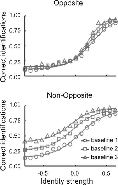
The final simulations address face identity aftereffects reported by Rhodes and Jeffery (2006). These findings have been widely cited as providing perhaps the most compelling behavioral evidence in favor of norm-based models over exemplar-based models (e.g., Jeffery et al., 2010; Jeffery & Rhodes, 2011; Rhodes & Leopold, 2011; Rhodes et al., 2005; Tsao & Freiwald, 2006). Their study design was an extension of the Leopold et al. (2001) paradigm, adding an additional control condition to more carefully assess the direction of aftereffects relative to the norm.

Just like the morph trajectories used in the Leopold et al. anti-face paradigm, Rhodes and Jeffery constructed “opposite” morph trajectories extending from four target faces (Dan, Jim, Rob, and Ted) through the average face, to an opposite-adaptor (anti-face) on the other side. However, in addition, Rhodes and Jeffery also constructed “non-opposite” morph trajectories between each of the four target faces and a non-opposite adaptor. These non-opposite faces were explicitly selected to be roughly the same perceptual distance from their respective target faces as their corresponding opposite adaptors. Opposite and non-opposite adaptors are illustrated in Figure 7a. Importantly, non-opposite trajectories do not pass through the norm.

Figure 7.

(a) Schematic face-space representation of the relationship between the stimuli in the Rhodes and Jeffery (2006) paradigm. Opposite morph-trajectories were constructed between each of the four target faces (only one shown here) and an opposite adaptor on the other side of the average face. Non-opposite morph-trajectories were constructed between each target face and a non-opposite adaptor. (b) Sensitivity to face identity with and without adaptation, shown for opposite (Top) and non-opposite (Bottom) morph-trajectories (data from Rhodes and Jeffery). Two conditions are shown: baseline responses (○), and responses following adaptation (●). The proportion of correct responses at each identity level has been averaged across the four identity trajectories and a best-fitting four parameter logistic function is shown for each condition.

As in Leopold et al. (2001), Rhodes and Jeffery (2006) examined face identity aftereffects following adaptation to each of the opposite adaptors along the corresponding trajectory from a given opposite adaptor to its matching target (equivalent to matching anti-face adaptation). However, in addition, identity aftereffects were also measured following adaptation to each of the non-opposite adaptors along the corresponding non-opposite trajectory from a given non-opposite adaptor to its matching target. So, whereas Leopold et al. examined adaptation to matching and non-matching adaptors along an opposite trajectory to the target, Rhodes and Jeffery examined adaptation to opposite and non-opposite adaptors along their corresponding opposite and non-opposite trajectories to the target.

Arguably, these additions to the experimental design by Rhodes and Jeffery provide a stronger test of an opposite perceptual bias than Leopold et al. (2001). It has been suggested that if adaptation results in a general perceptual bias, as commonly attributed to exemplar-based models, then there ought to be no difference between the aftereffects produced by adapting to opposite adaptors, as measured along the opposite morph-trajectories, and the aftereffects produced by adapting to non-opposite adaptors as measured along the non-opposite morph-trajectories. In contrast, if adaptation results in an opposite bias, as commonly attributed to norm-based models, then while opposite adaptors will bias identification of morphs on the opposite morph-trajectories directly towards the corresponding targets, non-opposite adaptors will not. This is because the targets are not opposite to the non-opposite adaptors.

Significantly for the norm vs. exemplar debate, the pattern of results reported by Rhodes and Jeffery (2006) was in line with the latter set of predictions, suggesting that adaptation is best described as an opposite bias with respect to a norm. As illustrated in Figure 7b, in the opposite adaptor condition, adaptation to the opposite adaptor significantly facilitated recognition of the target identity, as indicated by the shift in the psychometric function to the left. This is a replication of Leopold et al. (2001), where adaptation to a matching anti-face, say anti-Adam, facilitated identification of the target face Adam. However, while there is some facilitatory effect of adaptation in the non-opposite condition, it is substantially less, with the psychometric function only moving slightly leftwards relative to baseline.

While intuitions regarding predictions of norm-based and exemplar-based models may appear compelling, they must be explicitly tested by simulation. To simulate this paradigm, four target faces were selected and learned in the same way as the Leopold et al. paradigm. Similar to the earlier simulations, four opposite morph-trajectories were constructed for each target face, consisting of 15 identity levels created in steps of 0.1 between the 0.6 identity level (60% of the distance from the target face to the average face) and the -0.80 identity level on the other side of the average. The -0.80 identity level also served as the opposite adaptor. Next, a non-opposite adaptor was selected for each of the target faces to be an equal distance from the target as the opposite adaptor. Adapting the approach used in the Rhodes and Jeffery's experiment, the non-opposite adaptors were constructed by first measuring the Euclidean distances between the input-vectors of a set of 30 randomly selected faces and each of the four targets and then comparing these distances with the Euclidean distance between the corresponding opposite adaptor and the four targets in order to find the closest match. Having found a suitable non-opposite adaptor for each of the targets, a set of non-opposite trajectories was then created in the same way as for the opposite adaptors, defining the 0.0 point to be the same proportional distance between the target face and the non-opposite adaptor as the average face (0.0) on the opposite trajectory.

Following Rhodes and Jeffery (2006), the probability of a correct identification was recorded at each identity level on each of the four opposite and four non-opposite morph-trajectories both with and without prior adaptation. Figure 8a and 8c show a set of model predictions obtained from Gaussian (top row) and PCA-based (bottom row) versions of the three models (exemplar-based, traditional norm, and two pool), respectively. To obtain the displayed predictions, the probability of a correct response at each identity level was averaged across the four morph-trajectories, and then a four-parameter logistic function was fitted to the mean in each condition (Opposite Baseline, Non-Opposite Baseline, Opposite Adaptation, & Non-Opposite Adaptation). The parameters used to generate Figures 8a and 8c were identical to those used in the other simulations in this article.

Figure 8.

Qualitative and quantitative predictions from the three models on Rhodes and Jeffery's (2006) adaptation paradigm. Left: predictions from the exemplar-based model. Middle: predictions from the traditional norm-based model. Right: predictions from the two-pool norm-based model. (a) Representative quantitative predictions for the Gaussian versions of the three models. Each plot shows sensitivity to face identity with and without adaptation, shown for opposite (Top) and non-opposite (Bottom) morph-trajectories. Two conditions are shown: baseline responses (○), and responses following adaptation (●). The proportion of correct responses at each identity level has been averaged across the four identity trajectories and a best-fitting four parameter logistic function is shown for each condition. (b) Representative qualitative predictions from Gaussian versions of the three models for different parameter values. White squares represent no significant adaptation. Grey squares represent a qualitative agreement between the predictions and the findings in the literature. Black squares represent some qualitative disagreement between the model predictions and Rhodes and Jeffery's findings. (c) Representative quantitative predictions from the PCA versions of the three models.

It is clear that both the Gaussian and PCA-based versions of the exemplar and two-pool model captured the essential features of Rhodes & Jeffery's (2006) results. In the opposite condition, where the morph-trajectories pass directly through the average face, adaptation facilitates target identification, indicated by a significant shift in the psychometric function to the left. While adaptation also facilitated target identification in the non-opposite condition, the shift in the psychometric function is smaller, as observed empirically. Unlike the exemplar and two-pool models, it appears that, in the traditional norm-based model, adaptation resulted in roughly the same amount of adaptation in the opposite and non-opposite conditions.

Like the simulations of the Leopold et al. (2001) paradigm, Gaussian versions of the three models were also tested across a wide range of parameters (Table 1) and the results were aggregated to create a qualitative map for each model (Figure 8b). In this case, three criteria were considered, each evaluated using two-tailed t-tests (p < 0.01). First, for both the opposite and non-opposite conditions, we tested whether the predicted identification thresholds (taken at the inflection point) were significantly lower following adaptation to the respective opposite or non-opposite adaptor. This would indicate that adaptation facilitated the correct identification of the target as it did in Rhodes and Jeffery's (2006) study. Second, and perhaps more importantly, we tested whether there was significantly more adaptation predicted in the opposite than the non-opposite condition.

The combination of these three criteria provided a measure of the qualitative account of Rhodes and Jeffery (2006). The results of the qualitative fit were converted into qualitative maps (Figure 8b) and coded as follows: A set of parameters was only considered to provide a qualitative match to the observed data if all three criteria were met. That is, that adaptation resulted in a reduction in the identification threshold along both the opposite and the non-opposite morph trajectories and there was a significantly greater reduction in identification threshold along the opposite morph trajectory as compared to the non-opposite trajectory. If all three criteria were met then the parameter combination was coded as a qualitative match, represented by gray squares in Figure 8b. For a square to be coded as white, all three criteria had to be non-significant (i.e., no significant differences at all). All other combinations of results were coded as black, which meant that there were significant differences and at least one qualitatively incorrect prediction. We did also explore the three criteria individually; however, unless otherwise mentioned, the qualitative maps in Figure 8b provide an accurate representation of the findings regardless of how we parse them. As was done earlier, the maps were collapsed across values of ϕ and θ because those parameter values did not affect the general pattern observed in the qualitative maps.

The qualitative predictions of the exemplar and two-pool model were fairly consistent across parameter values, with many combinations of parameters leading to qualitatively correct predictions. As with the simulations of Leopold et al., for the exemplar model, there were some parameter combinations that predicted no significant effects. For both the exemplar and two-pool maps, there were some cases where both models made qualitatively incorrect predictions (black squares). Unpacking the source of these mispredictions a bit, for both models there were borderline cases where there was significant adaptation in the opposite condition but insufficient power to judge the opposite and non-opposite condition to be significantly different from one another. Interestingly, many of these mispredictions are for simulations assuming face spaces having only two dimensions. Nearly all intuitions about the effects of adaptation on face recognition are generated using illustrations drawn in two dimensions. While no one thinks that face space is only two dimensional, it is clear that intuitions generated in two dimensions, as well as simulations assuming two dimensions, do not necessarily generalized to more realistic face-space representations with more dimensions.

For the traditional norm-based model, no combination of parameters produced a qualitatively correct prediction, as reflected by the complete tiling of black squares. The traditional norm-based model generally predicted that there would be as much, and sometimes more, adaptation in the non-opposite condition, which is opposite to the finding reported by Rhodes and Jeffery. The specific qualitative prediction did depend on the particular value of the scaling parameter ϕ; because the magnitude of the predicted aftereffect in the opposite and non-opposite was very similar, the precise shape of the psychometric function could be pushed around by the value of ϕ, making one condition or another appear to show more or less adaptation. Thus, it appears that the traditional norm-based model cannot predict an “opposite bias” whereas both the exemplar-based and two-pool models can.

These simulations also allow us to address another property of the observed empirical data that has been taken as support for norm-based models. Examine the pre-adaptation baselines for the opposite and non-opposite conditions in Rhodes & Jeffery's data (Figure 7b). In the opposite condition, identification at 0.0 identity strength (the average face) is at chance (25%) and identification at negative identity levels (anti-faces) on the opposite side of the average face from the target are below chance. Rhodes and Jeffery (2006) contrasted this with identification at comparable identity strengths in the non-opposite condition, test faces of comparable distance from the target face along the non-opposite trajectory. In the non-opposite condition, identification at the comparable 0.0 identity strength is substantially above chance (greater than 25%). This finding has been interpreted as further support for a norm-based account because faces on the opposite side of the average face are also psychologically opposite, in way predicted by norm-based models: “... for opposite baselines ... performance on the 0% targets, i.e., the anti-faces, was below chance (25%), indicating a reluctance to choose the computationally opposite identity when faced with an unlearned identity. No such reluctance was seen for non-opposite identities. This result provides further evidence that computationally opposite, but not other equally dissimilar, but non-opposite, faces are perceived as opposites and that identity is coded relative to the average” (Rhodes & Jeffery, 2006, p. 2981).

It should be clear from Figure 8b that all three models predict this difference. Given that there is no explicit sense in which a face is “opposite” in an exemplar-based model, it is worth reconsidering Rhodes and Jeffery's interpretation since it is not unique to norm-based models. In fact, the prediction can be quite simply explained by the fact that all four opposite morph-trajectories pass through the exact same point at 0.0 identity strength. All four trajectories pass through the exact same average face. Therefore, it is impossible for baseline performance to be anything but chance without adaptation. In contrast, the four non-opposite trajectories do not pass through a single point. While all four non-opposite trajectories have a 0.0 identity strength, each of those 0.0 points corresponds to a completely different face. Above chance performance at the 0.0 identity strength is entirely possible depending on how the space is carved up into identity regions during learning.

We do also note that the left asymptote of the psychometric function (negative identity strengths) in the non-opposite condition is quantitatively higher in the observed data than in some of the model predictions (especially the Gaussian model). As suggested by Rhodes and Jeffery, potential learning along non-opposite morph trajectories could cause this increased asymptote, which we address next.

Learning Along Opposite and Non-Opposite Morph Trajectories

In the final set of simulations we address a curious observation made by Rhodes and Jeffery (2006) regarding the learnability of morphs along opposite and non-opposite morph trajectories. In addition to the opposite and non-opposite baseline conditions illustrated in Figure 7b, Rhodes and Jeffery also included a “pre-adaptation” baseline condition. For the opposite trajectories, there was no difference between pre-adaptation and post-adaptation baselines. However, for non-opposite trajectories, there was a significant difference between pre-adaptation and post-adaptation. Participants may have learned about identities over the course of the experiment. Because of this learning effect, when analyzing the data simulated in the previous section, Rhodes and Jeffery compared adaptation blocks to the post-adaptation baseline, not to pre-adaptation baseline: “Given the strong learning effect for non-opposite trajectories the identity aftereffect cannot be measured by comparing adaptation thresholds with pre-adaptation baseline thresholds” (Rhodes & Jeffery, p. 2981).

They confirmed that this was a learning effect by testing additional participants over several days of baseline testing, showing significant changes in identification functions over learning for non-opposite morph-trajectories but not opposite morph-trajectories. Figure 9 displays the baseline functions observed by Rhodes and Jeffery over the course of three sessions (baseline 1, baseline 2, and baseline 3). Clearly, while there was little change in the opposite baseline across the three sessions, there was substantial change in the non-opposite baseline. Namely, with each subsequent session the identification threshold in the non-opposite baseline was considerably reduced. Moreover, the psychometric functions appear to have leveled off at its left asymptote (negative identity strength) at an above chance level of performance that is further above chance with further learning.

Figure 9.

Baseline sensitivity to face identity in three consecutive sessions observed by Rhodes and Jeffery (2006) for opposite (Top) and non-opposite (Bottom) morph-trajectories. Three conditions are shown: performance in session 1 (○), baseline performance in session 2 (□), and baseline performance in session 3 (▲). The proportion of correct responses at each identity level has been averaged across the four identity trajectories and a best-fitting four parameter logistic function is shown for each condition.

To account for the learning effect, Rhodes and Jeffery (2006) suggested that perhaps “greater visibility” of the target identities in the non-opposite morphs allowed participants to associate them with the relevant target identities more readily than in the non-opposite condition. This interpretation is based on an idea that in a norm-based model the adaptor faces will be opposite identities and will thus mask the target identity more than the non-opposite faces. In other words, this learning effect along non-opposite but not opposite morph-trajectories could provide further evidence for norm-based over exemplar-based models.

However, as we noted in discussing the results of the previous simulation, there is another conspicuous difference between opposite and non-opposite morph trajectories. Unlike opposite trajectories, which all pass through the average face, non-opposite morph trajectories do not all have to pass through a single point. It is logically impossible for participants to have above chance performance on the average face, regardless of the amount of learning. In contrast, as the equivalent point on the non-opposite trajectories corresponds to four entirely different faces, it is at least theoretically possible to learn to which identity they might best correspond.

Following this logic, we tested whether the learning effect observed by Rhodes and Jeffery (2006) could, at least in principle, be explained by a change in the way that the decision space is carved up over learning. To do this, we first trained the three models (exemplar-based, traditional norm-based and two-pool) on the four target identities, using the exact same procedures described for the previous simulations, to obtain the equivalent of pre-adaptation baseline identification probabilities along the opposite and non-opposite trajectories (baseline 1). Next, using a fairly small learning rate, the models were further trained on the full range of faces along the opposite and non-opposite trajectories for 200 epochs and another baseline was recorded along opposite and non-opposite trajectories (baseline 2). This was then repeated for another 200 epochs and another baseline was obtained (baseline 3). To be clear, for simplicity here we have modeled learning in the neural network as consequence of explicit feedback, whereas participants in Rhodes and Jeffery (2006) received no feedback regarding the identity of morph faces along any of the trajectories. We would need a far more elaborate model of how self-generated labeling of test faces might be used to guide learning to fully model these learning effects. We only intend these simulations as a demonstration of the potential effect that learning, whether explicit or implicit, can have given a particular model and space of stimuli.

Figure 10 shows the simulation results of varying amounts of learning on baseline identification performance for the Gaussian version of all three face-space models. As shown in the top row, just like Rhodes and Jeffery, for all three models, there was little or no effect of additional learning for opposite trajectories. In fact, with slightly higher learning rates there was a slight steepening of the psychometric function, as can be observed in Rhodes and Jeffery's data (Figure 9). As shown in the bottom row, just like Rhodes and Jeffery, additional learning had a significant affect on non-opposite trajectories. But those affects are not specific to norm-based models. Exemplar-based models predict them as well. As we discussed earlier, for all four opposite trajectories, the 0.0 identity strength is the same face. There is no way that any additional learning along those morph trajectories could move the identification probability for that face away from chance. By contrast, for the four non-opposite trajectories, the corresponding 0.0 identity strength is different. So even modest learning along those trajectories, perhaps caused by self-generated labeling during testing (see also Palmeri & Flanery, 1999, 2002), could cause the identification probabilities for those ostensibly 0.0 identity strength faces to shift to be greater than chance. There is nothing structural about the distribution of faces along the four non-opposite trajectories to prevent that from happening.

Figure 10.

Baseline sensitivity to face identity in three consecutive sessions predicted by the Gaussian version of the three models for opposite (Top) and non-opposite (Bottom) morph-trajectories. Three conditions are shown: baseline performance after 200 epochs (○), baseline performance after 400 epochs (□), and baseline performance after 600 epochs (▲). The proportion of correct responses at each identity level has been averaged across the four identity trajectories and a best-fitting four parameter logistic function is shown for each condition.

General Discussion

Face identity aftereffects have been researched extensively for over a decade. Identification of a face is perceptually biased by adaptation to an anti-face on the opposite side of the average face (e.g., Leopold et al., 2001). But identification is far less biased by adaptation to an equidistant, non-opposite face that is not on the other side of the average face (e.g., Rhodes & Jeffery, 2006). Aftereffects like this have been taken as strong evidence for an explicit representation of the average face – the face norm. They have also been taken as strong evidence against models without explicit norms, including exemplar-based models. However, to our knowledge, there have been no past attempts to formally test predictions of norm-based or exemplar-based models regarding face identity aftereffects. Contrary to a dominant view in the literature, we found that both a two-pool norm-based model and an exemplar-based model made qualitatively accurate predictions of the most widely-cited face identify aftereffect paradigms.

To summarize, we implemented a traditional norm-based model, a two-pool norm-based model, and an exemplar-based model of face space based on past formalizations and common descriptions in the face recognition literature. All three models shared the same assumptions about the perceptual input representation, the decisional output mechanism, and the learning between face space and an identification decision. For each of these models, we implemented one version that simply assumed that each face was randomly sampled from a multivariate normal distribution and another version that assumed a PCA-based perceptual front-end that created a face representation from a face image. We reported simulation results using a fixed set of parameter values that provided reasonable quantitative predictions and for some key findings we also reported qualitative predictions across a broad range of parameter values.

We tested predictions of each model in three different paradigms. The first was one of the original demonstrations of the face identity aftereffect (Leopold et al., 2001), finding that adaptation to a matching (opposite) anti-face produced an aftereffect while adaptation to a non-matching (non-opposite) anti-face did not. The second was a demonstration of how adaptor location affects the magnitude of the face identity aftereffect (Leopold & Bondar, 2005), finding that adaptation to an average face produced little or no aftereffect compared to adaptation to true anti-faces on the other side of the average. The third equated distance for opposite and non-opposite adaptors (Rhodes & Jeffery, 2006), finding qualitative and quantitative differences between opposite anti-face adaptation that respects the norm compared to non-opposite adaptation that does not.

We found that both an exemplar-based model and a two-pool norm-based model accounted well for the behavioral data but a traditional norm-based model often did not. These findings are important in the context of the current face recognition literature. Many recent reviews (e.g., Jeffery & Rhodes, 2011; Leopold & Bondar, 2005; Rhodes & Leopold, 2011; Rhodes et al., 2005; Tsao & Freiwald, 2006; Tsao & Livingstone, 2008) cite the difference in adaptation for opposite versus non-opposite adaptors as compelling evidence in favor of a norm-based account and against an exemplar-based account of face space representation. Findings that the magnitude of aftereffects increase as a function of adaptor distance from the average has been taken as evidence for norms in face identification by adults (e.g., Leopold & Bondar, 2005), face identification by children (e.g., Jeffery et al., 2010), and emotion perception by adults (e.g., Skinner & Benton, 2010). These theoretical claims may need to be reevaluated.

Our model simulations reinforce a common refrain on the virtues of computational modeling that “surprises are likely when the model has properties that are inherently difficult to understand, such as variability, parallelism, and nonlinearity” (Hintzman, 1990). Clearly, common intuitions about predictions of norm-based and exemplar-based models of face identity aftereffects do not always align with the actual predictions of these models when they are explicitly formalized and simulated. Why are those intuitions wrong?

In part this comes from a common, but sometimes erroneous, attempt to map a particular behavioral effect directly onto a particular psychological mechanism. It is clear that effects of adaptation vary with respect to the average face. Opposite adaptors are more effective than non-opposite adaptors and adaptation with the average itself is ineffective compared to adaptation with an opposite adaptor. But sensitivity to the location of the average does not imply that the average, or norm, must be explicitly represented. The fact that prototype effects do not by themselves imply prototype representations has been demonstrated many times in the category learning literature (e.g., Busemeyer, Dewey, & Medin, 1984; Nosofsky, 1992; Palmeri & Nosofsky, 2001). Such observations from category learning are commonly cited in the face recognition literature, yet sensitivity of face identity aftereffects to the average continues to be described as compelling evidence in favor of an explicit representation of faces in reference to a face prototype or norm.

Explicit simulation and prediction requires that multiple psychological mechanisms be modeled, even if some may not be of direct theoretical interest. While we maintained relative simplicity in our modeling, in order to simulate face identity aftereffects, we had to be explicit about how faces are perceptually represented, how face space is represented, how face space representations are associated with learned face identities, and how identification decisions are made. While the empirical focus of face adaptation experiments is typically on face representations, as was our theoretical focus as well, all of these psychological mechanisms are used by any subject in any experiment to identify a face. Some of these may seem theoretically “uninteresting”, but they are all important to predict face identification performance. We chose to keep these “uninteresting” psychological mechanisms constant across different assumptions regarding face space representation, but we needed them all in order to simulate behavior. Intuitions based solely on visual inspection of simplified illustrations of face space, without considering how those face space representations are used to make learned identification decisions, seems inadequate (see Palmeri & Cottrell, 2010).

Even intuitions focused entirely on face space can fail when is comes to generalizing from simple two-dimensional illustrations to more realistic representations assuming higher dimensionality. In general it is difficult to intuit the true nature of a high-dimensional space (e.g., DiCarlo & Cox, 2007). For example, in one dimension, random samples from a Gaussian distribution cluster around the mean, as expected. The same is true in two dimensions. With many dimensions, random samples along any one dimension cluster around the mean along that dimension, but those samples do not cluster in the center of the space like they do in one or two dimensions (see Burton & Vokey, 1998). Indeed, any given face probably has a value more toward the tail of the distribution along at least one dimension. Consider an extreme case and imagine a face space with several hundred dimensions. In order for most faces to be clustered in the center of that multidimensional space, like they do in one or two dimensions, no face could ever have an extreme value along any of those several hundred dimensions. The likelihood of that ever happening is beyond remote. Every face is unique in its own unique way. So illustrations of exemplar models in two dimensions, including those we adapted for illustration in Figure 2, simply do not generalize well to multiple dimensions. No one thinks that face space is two-dimensional but few people can imagine spaces with more than three dimensions. Explicit simulations of models assuming multidimensional face spaces are not merely exercises in added rigor, but are necessary to generate reasonable predictions.

Considering the distribution of faces in multidimensional face space, in one sense, the norm is represented “implicitly” in our simulations of exemplar-based models, if only in the restricted sense that the multidimensional distribution of face representations are organized around a hypothetical average face. In the Gaussian version, this is merely a consequence of assuming a unimodal, multivariate normal distribution of faces. In the PCA-based version, PCA dimensions are extracted that maximize variance in particular directions in image space, and tend to unimodal multivariate distributions as well. The average is a matter of statistics, not explicit representation. Exemplar models are sensitive to the parametric statistical structure of the space of examples learned, but they do not need to represent explicitly parametric measures, such as the average, or norm, of the space itself.

By contrast, intuitions about predictions of exemplar models are often based on a uniform tiling of exemplars in face space, with our illustrations in Figures 2 and 3 intentionally adapted from published work describing those predictions (e.g., Susilo et al. 2010b). Realistic exemplar models are multidimensional, not one- or two-dimensional. Realistic exemplar models assume multivariate statistical distributions of exemplars that reflect the image statistics of a large sample of experienced faces. These distributions have modes often centered on an average face. They also have tails with limited extent. It is common to describe adaptation predicted by exemplar models as a uniform perceptual bias that is equipotent in all directions in face space, but that would only be true if exemplar representations were uniformly tiled over an infinite extent of face space. Considering jointly the multidimensionality, the mode, and limited tails of the distribution of exemplars in face space, the fact that exemplar-based models can naturally make predictions that are similar to models assuming an explicit representation of the norm may be less surprising.

It also became clear in our explicit simulations that some of the behavioral sensitivity of adaptation with respect to the average face may be a consequence of experimental design as much as psychological representation. Recall that Rhodes and Jeffery (2006) observed significant differences in the effects of adaptation and learning on identification thresholds and shapes of psychometric functions depending on whether the adaptor was opposite or non-opposite. While morph trajectories for both opposite and non-opposite conditions had a 0.0 identity strength defined along their continua, these were qualitatively different. For the four morph trajectories defined with respect to the four opposite adaptors, the 0.0 identity strength was the exact same face, the average face. However, for the four morph trajectories defined with respect to the four non-opposite adaptors, the 0.0 identity strength was a completely different face. While these faces may be labeled “0.0 identity strength” in both conditions, they are experimentally quite different. There is really no viable model of face recognition that would not predict qualitative differences between opposite and non-opposite morph trajectories since identification of the average face without adaptation must be at chance. This is not necessarily a consequence of a special psychological status for the average face, but a mathematical consequence of the exact same face being equally likely, on average, to be identified with one of the four learned names.

As with any project using simulations, whether formalizing verbal theoretical descriptions or generalizing existing computational models to new domains, it is likely that certain aspects of the specific implementations can and will be disputed. This is a strength, not a weakness, of a model-based approach. Because the underlying assumptions are made explicit, they can be critically evaluated and future work can compare our formalizations against alternative computational instantiations. Explicitly defining models opens up the possibility of designing new behavioral experiments that can better differentiate models. This has been true in the category learning literature, where prototype and exemplar-based models have been extensively contrasted in behavioral experiments informed by predictions of computational models. Face recognition could be similarly informed by models.

The models implemented in this article were guided by our understanding of the verbal descriptions in the face recognition literature and by previous models that have been instantiated in both the categorization and face recognition literatures. In the paragraphs that follow, we address some of the potentially controversial assumptions of the models we formalized and tested, discuss limitations of our work, and suggest further avenues for research.

Anyone with some knowledge of the category learning literature may recognize that our instantiation of prototype and exemplar models makes assumptions somewhat different from common category learning models (e.g., Kruschke, 1992; Nosofsky, 1986; Palmeri, 1997). To begin with, the norm versus exemplar debate in the face recognition literature is not precisely the same as the prototype versus exemplar debate in the categorization literatures. In categorization, prototype models assume that a category is represented by its prototype, that the prototype embodies the representation of a category. In face recognition, norm models assume that individual faces in face space are represented with respect to the norm. Similar, but not the same.

In addition, for exemplar models, rather than assume that every newly learned face has its own unique exemplar representation in face space, we assumed that newly learned faces have a distributed representation based on their similarity to previously learned faces in face space. While different from some exemplar-based category learning models, this assumption is similar to some object recognition models that have an object space akin to our face space (e.g., Edelman, 1999; Riesenhuber & Poggio, 1999; see also Palmeri & Tarr, 2008; Palmeri et al., 2004). This also seemed to be a reasonable assumption given that in the face identity aftereffect experiments, the four target faces were completely novel at the start of the experiment and there was not much training on those faces before the adaptation trials began. While clearly participants are able to create memories for those learned faces and associate names with them, it may well be that new face-space representations are not created for faces unless they are quite familiar. That said, we did test versions of the model assuming that every learned face gets its own unique exemplar representation, observing no difference in qualitative predictions.

Perhaps one controversial assumption in our model simulations concerns the locus of adaptation effects. In all three models, adaptation was implemented within the face-space layer itself, adapting face representations in proportion to their activation by the adaptor. This seems reasonable given that face identity adaptation effects have been used as evidence regarding the nature of face-space representations, whether they are norm-based or exemplar-based (e.g. Jeffery et al., 2010; Leopold & Bondar, 2005; Leopold et al., 2001; Rhodes & Leopold, 2011; Rhodes & Jaquet, 2011; Rhodes, et al., 2011; Rhodes & Jeffery, 2006; Rhodes et al., 2010; Rhodes et al., 2005; Tsao & Freiwald, 2006). Furthermore, many illustrations of adaptation effects have used 2D face-space representations (Robbins et al., 2007; Rhodes & Jeffery, 2006; Rhodes, 2005), which could suggest that adaptation is acting within the face-space layer itself. Face identity aftereffects have been characterized as high-level aftereffects (Leopold & Bondar, 2005; Leopold et al., 2001), to distinguish them from low-level sensory aftereffects. But how high is “high”?

It is not unreasonable to imagine that face identity aftereffects could reflect adaptation at multiple levels of processing within the visual system (Hills et al., 2010). Adaptation of face-space representations is only one possible locus. Indeed, some have suggested that adaptation might take place at the level of the dimensional representations, not the face representations (e.g., Rhodes et al., 2005). A hybrid model is possible, where the dimensions of face space are encoded by opponent pools reflecting an implicit or explicit norm along that dimension and faces in face space are encoded by something more akin to exemplars. But developing and testing a model of that sort goes well beyond the scope of this article. So then the question may not be whether face space is represented by norms or exemplars, but whether the dimensions of face space are represented by norms or multichannel coding (e.g., Robbins et al., 2007; Susilo et al., 2010b). This is an important question. But exemplar models concern representations of objects or faces, not representations of dimensions.

Our simulations have been limited to face identity aftereffects. Subjects learn the identities of faces and adaptation systematically changes how other faces within face space are identified. Other adaptation aftereffects concern judgments about the configuration of faces (e.g., Webster & MacLeod, 2011) such as whether the separation of the eyes is more or less than average (Robbins et al., 2007; Susilo et al., 2010b). Indeed, the literature on face adaptation is vast (e.g., see Rhodes & Leopold, 2012, for a recent review) and we have only scratched the surface. Modeling these figural aftereffects would require a more precise model of how faces are represented dimensionally than the models we tested here. Our Gaussian versions were completely agnostic to how face dimensions are created, simply assuming that a novel face is a random sample from a multivariate Gaussian distribution. Our PCA-based versions did go from a face image to a face representation, but by its very nature, PCA representations have no explicit representation of face parts. There is no explicit representation, for example, of the distance between two eyes in a PCA-based representation since PCA representations (so-called eigenfaces) are inherently holistic. For face identity aftereffects, this does not matter. For figural aftereffects, there must be a way to interrogate representations of parts or features, not just representations of the whole. Our models focused on face space and how decisions are made based on activations in face space.

Just about every paper on face identity aftereffects has acknowledged the decades-old prototype versus exemplar debate in the categorization literature. But most of these papers also argue that face identity aftereffects provide compelling evidence in favor of norm-based models and against exemplar-based models. These arguments are often grounded in intuitive descriptions, sometimes supplemented by illustrations of face space in one or two dimensions. Our explicit modeling challenges these intuitions and illustrations. Both an exemplar-based and a two-pool version of a norm-based model accounted for three important face identity aftereffects, but a traditional norm-based model did not.⁴ Illustrations in one or two dimensions may be easy to understand, but they do not map well onto spaces with more dimensions. Explicit computational models can assume multiple dimensions in a way that more closely mirrors the assumptions most people have about face space. Verbal descriptions about how adaptation might affect face space often focus entirely on individual face representations and their possible contributions to identification. Explicit computational models can assume parallel activation of multiple faces that contribute in concert to face identification in a way that more closely mirrors how most people think face recognition actually happens. Descriptions and illustration focus on face space. Explicit computational models must assume not only face space and how it is activated by adaptors or test faces but must also assume explicit learning and decision mechanisms that use face space for identification. This conjoining of components can lead to predictions that are not obvious from intuitions about any particular component in isolation. Surprises are likely.

Appendix A

The PCA-based versions assume a very simple perceptual front end, allowing us to present each model with a face image. In our case, the images used to construct the PCA were 50 randomly selected, 256 × 256 pixel faces from the Max Planck Institute (MPI) Database (Troje & Bulthoff, 1996). In terms of raw pixel intensities, each face is represented in a 256 × 256 = 65,536 dimensional space. PCA performs dimensionality reduction, identifying a new set of components (dimensions) that explain the variance across the 50 faces. The first component accounts for the greatest amount of variance across the face images, the next component the second highest amount of variance, and so forth. While in the limit, there could be as many components (dimensions) in the PCA space as the original intensity space, the power of PCA is that it reduces dimensions. In our case, the number of PCA components we assumed depended on the number of face-space dimensions (n) being assumed in a given simulation.

Some models assuming PCA have performed PCA on raw pixel intensities (e.g., O'Toole et al., 1993) or on gabor-filtered images (e.g., Dailey & Cottrell, 1999; Richler et al., 2007; see also Palmeri & Cottrell, 2010). We instead followed Burton et al., (1999), who suggested an way to represent face images with PCA by processing the shape information and the texture (intensity) information separately; because we were primarily interested in representing changes in face shape along morph trajectories, we ignored texture information. Following Burton et al., to extract face shape, a set fiducial markers were placed at key face landmarks (170 locations in total). The landmarks were placed by hand and their locations were chosen to outline the shape of the face and various key features (e.g., eyes, nose, mouth, etc.), with a given landmark placed at a corresponding location on each face. The full matrix of landmarks, defined by their x,y coordinates, on every face in the training set was analyzed using PCA.

Appendix B

Face images were presented to the three PCA-based versions of the models, just like face images would be presented to a participant in an experiment (see Appendix A). Therefore, it was necessary to create face stimuli along morph trajectories, just like they would need to be created for a behavioral experiment. We adapted procedures used in the previous face identity aftereffect experiments simulated in our paper, that we briefly summarize here. As described in the main text, a set of four target faces (i.e., Adam, Jim, John, and Henry) was first randomly selected. In addition, a set of thirty additional faces was randomly selected from which to construct an average face. Fiducial points (x,y) were placed on the 34 faces by hand in locations corresponding to the fiducial points used in the PCA (see Appendix A). Because the PCA-based front end only operated on the location of these fiducial marks, the rest of the image information was discarded. The average face then corresponds to the average x,y image locations of fiducial markers on the set of thirty faces. To construct a morph trajectory between a target face and the average face, the x,y locations of the fiducial markers were adjusted in proportion to the difference between the target and average and the value of the identity strength. To continue the morph trajectory through the average face to an opposite face, the locations of the fiducial markers were simply extrapolated along the same vector they were going to the average face.

References

- Ashby FG, editor. Multidimensional models of perception and cognition. Lawrence Erlbaum Associates, Inc.; Hillsdale, NJ: 1992. [Google Scholar]
- Benson PJ, Perrett DI. Visual processing of facial distinctiveness. Perception. 1994;23:75–93. doi: 10.1068/p230075. [DOI] [PubMed] [Google Scholar]
- Busemeyer JR, Dewey GI, Medin DL. Evaluation of exemplar-based generalization and the abstraction of categorization information. Journal of Experimental Psychology: Learning, Memory, and Cognition. 1984;10:638–648. doi: 10.1037//0278-7393.10.4.638. [DOI] [PubMed] [Google Scholar]
- Burton AM, Bruce V, Dench N. What's distinctive about a distinctive face? The Quarterly Journal of Experimental Psychology. 1994;47A:119–141. doi: 10.1080/14640749408401146. [DOI] [PubMed] [Google Scholar]
- Burton AM, Bruce V, Hancock PJB. From pixels to people: A model of familiar face recognition. Cognitive Science. 1999;23:1–31. [Google Scholar]
- Burton AM, Vokey JR. The face-space typicality paradox: Understanding the faces-space metaphor. The Quarterly Journal of Experimental Psychology. 1998;51A:475–483. [Google Scholar]
- Dailey MN, Cottrell GW. Organization of face and object recognition in modular neural network models. Neural Networks. 1999;12:1053–1073. doi: 10.1016/s0893-6080(99)00050-7. [DOI] [PubMed] [Google Scholar]
- DiCarlo JJ, Cox DD. Untangling invariant object recognition. Trends in Cognitive Sciences. 2007;11:333–341. doi: 10.1016/j.tics.2007.06.010. [DOI] [PubMed] [Google Scholar]
- Edelman S. Representation and recognition in vision. MIT Press; Cambridge, MA: 1999. [Google Scholar]
- Farrell S, Lewandowsky S. Computational models as aids to better reasoning in psychology. Current Directions in Psychological Science. 2010;19(5):329–335. [Google Scholar]
- Gibson JJ, Radner M. Adaptation, after-effect, and contrast in the perception of tilted lines. I. Quantitative studies. Journal of Experimental Psychology. 1937;20:453–467. [Google Scholar]
- Giese MA, Leopold DA. Physiologically inspired neural model for the encoding of face spaces. Neurocomputing. 2005;65-66:93–101. [Google Scholar]
- Griffin JH, McOwan WP, Johnston A. Relative faces: Encoding of family resemblance relative to gender means in face space. Journal of Vision. 2011;11(12):1–11. doi: 10.1167/11.12.8. [DOI] [PubMed] [Google Scholar]
- Grill-Spector K, Henson R, Martin A. Repetition and the brain: neural models of stimulus-specific effects. Trends in Cognitive Sciences. 2006;10(1):14–23. doi: 10.1016/j.tics.2005.11.006. [DOI] [PubMed] [Google Scholar]
- Hancock PJB, Little A. Adaptation may cause some of the face caricature effect. Perception. 2011;40(3):317–322. doi: 10.1068/p6865. [DOI] [PubMed] [Google Scholar]
- Hills PJ, Elward RL, Lewis MB. Cross-modal face identity aftereffects and their relation to priming. Journal of Experimental Psychology: Human Perception and Performance. 2010;36(4):876–891. doi: 10.1037/a0018731. [DOI] [PubMed] [Google Scholar]
- Hintzman DL. Human learning and memory: Connections and dissociations. Annual Review of Psychology. 1990;41:109–139. doi: 10.1146/annurev.ps.41.020190.000545. [DOI] [PubMed] [Google Scholar]
- Jeffery L, McKone E, Haynes R, Firth E, Pellicano E, Rhodes G. Four to-six-year-old children use norm-based coding in face-space. Journal of Vision. 2010;10(5):1–19. doi: 10.1167/10.5.18. [DOI] [PubMed] [Google Scholar]
- Jeffery L, Rhodes G. Insights into the development of face recognition mechanisms revealed by face aftereffects. British Journal of Psychology. 2011;102:799–815. doi: 10.1111/j.2044-8295.2011.02066.x. [DOI] [PubMed] [Google Scholar]
- Jiang F, Blanz V, O'Toole AJ. Three-dimensional information in face representations revealed by identity aftereffects. Psychological Science. 2009;20(3):318–325. doi: 10.1111/j.1467-9280.2009.02285.x. [DOI] [PubMed] [Google Scholar]
- Jiang X, Rosen E, Zeffiro T, VanMeter J, Blanz V, Riesenhuber M. Evaluation of a shape-based model of human face discrimination using fMRI and behavioral techniques. Neuron. 2006;50:159–172. doi: 10.1016/j.neuron.2006.03.012. [DOI] [PubMed] [Google Scholar]
- Kruschke JK. ALCOVE: An exemplar-based connectionist model of category learning. Psychological Review. 1992;99(1):22–44. doi: 10.1037/0033-295x.99.1.22. [DOI] [PubMed] [Google Scholar]
- Lee KJ, Perrett DI. Presentation-time measures of the effects of manipulations in colour space on discrimination of famous faces. Perception. 1997;26(6):733–752. doi: 10.1068/p260733. [DOI] [PubMed] [Google Scholar]
- Leopold DA, Bondar I. Adaptation to complex visual patterns in humans and monkeys. In: Clifford CWG, Rhodes G, editors. Fitting the mind to the world: Adaptation and after-effects in high-level vision. Oxford University Press; Oxford: 2005. pp. 213–240. [Google Scholar]
- Leopold DA, O'Toole AJ, Vetter T, Blanz V. Prototype-referenced shape encoding revealed by high-level aftereffects. Nature Neuroscience. 2001;4(1):89–94. doi: 10.1038/82947. [DOI] [PubMed] [Google Scholar]
- Lewis MB. Face-space-R: Towards a unified account of face recognition. Visual Cognition. 2004;11:29–69. [Google Scholar]
- Lewis MB, Johnston RA. Understanding caricatures of faces. Quarterly Journal of Experimental Psychology. 1998;51A:321–346. doi: 10.1080/713755758. [DOI] [PubMed] [Google Scholar]
- Lewis MB, Johnston RA. A unified account of the effects of caricaturing faces. Visual Cognition. 1999;6:1–41. [Google Scholar]
- Loffler G, Yourganov G, Wilkinson F, Wilson HR. fMRI evidence for the neural representation of faces. Nature Neuroscience. 2005;8:1386–1390. doi: 10.1038/nn1538. [DOI] [PubMed] [Google Scholar]
- Luce RD. Detection and recognition. In: Luce RD, Bush RR, Galanter E, editors. Handbook of Mathematical Psychology, I. Wiley; New York: 1963. pp. 103–189. [Google Scholar]
- Mack ML, Palmeri TJ. Modeling categorization of scenes containing consistent versus inconsistent objects. Journal of Vision. 2010;10(3):11, 1–11. doi: 10.1167/10.3.11. [DOI] [PubMed] [Google Scholar]
- Mather G, Verstraten F, Anstis S, editors. The Motion Aftereffect: A Modern Perspective. MIT Press; Cambridge, MA: 1998. [DOI] [PubMed] [Google Scholar]
- Nishimura M, Doyle J, Humphreys K, Behrmann M. Probing the face space of individuals with prosopagnosia. Neuropsychologia. 2010;48:1828–1841. doi: 10.1016/j.neuropsychologia.2010.03.007. [DOI] [PubMed] [Google Scholar]
- Nishimura M, Maurer D, Jeffery L, Pellicano E, Rhodes G. Fitting the child's mind to the world: adaptive norm-based coding of facial identity in 8-year olds. Developmental Science. 2008;11(4):620–627. doi: 10.1111/j.1467-7687.2008.00706.x. [DOI] [PubMed] [Google Scholar]
- Nishimura M, Robertson C, Maurer D. Effect of adaptor duration on 8 year olds’ facial identity aftereffects suggests adult-like plasticity of the face norm. Vision Research. 2011;51:1216–1222. doi: 10.1016/j.visres.2011.03.013. [DOI] [PubMed] [Google Scholar]
- Nosofsky RM. Attention, similarity, and the identification-categorization relationship. Journal of Experimental Psychology: General. 1986;115(1):39–57. doi: 10.1037//0096-3445.115.1.39. [DOI] [PubMed] [Google Scholar]
- Nosofsky RM. Exemplar-based approach to relating categorization, identification, and recognition. In: Ashby FG, editor. Multidimensional models of perception and cognition. Scientific psychology series. Lawrence Erlbaum Associates, Inc.; Hillsdale, NJ: 1992. pp. 363–393. [Google Scholar]
- O'Toole AJ, Abdi H, Deffenbacher K, Valentin D. Low-dimensional representation of faces in higher dimensions of the face space. Journal of the Optical Society of America. 1993;10:405–411. [Google Scholar]
- Palermo R, Rivolta D, Wilson CE, Jeffery L. Adaptive face space coding in congenital prosopagnosia: Typical figural aftereffects but abnormal identity aftereffects. Neuropsychologia. 2011 doi: 10.1016/j.neuropsychologia.2011.09.039. [DOI] [PubMed] [Google Scholar]
- Palmeri TJ. Exemplar similarity and the development of automaticity. Journal of Experimental Psychology: Learning, Memory, and Cognition. 1997;23:324–354. doi: 10.1037//0278-7393.23.2.324. [DOI] [PubMed] [Google Scholar]
- Palmeri TJ, Cottrell GW. Modeling perceptual expertise. In: Gauthier I, Tarr MJ, Bub D, editors. Perceptual Expertise: Bridging Brain and Behavior. Oxford University Press; Oxford: 2010. pp. 197–244. [Google Scholar]
- Palmeri TJ, Flanery MA. Learning about categories in the absence of training: Profound amnesia and the relationship between perceptual categorization and recognition memory. Psychological Science. 1999a;10:526–530. [Google Scholar]
- Palmeri TJ, Flanery MA. Memory systems and perceptual categorization. In: Ross BH, editor. The Psychology of Learning and Motivation. Vol. 41. Academic Press; 2002. [Google Scholar]
- Palmeri TJ, Nosofsky RM. Central tendencies, extreme points, and prototype enhancement effects in ill-defined perceptual categorization. Quarterly Journal of Experimental Psychology: Human Experimental Psychology. 2001;54A(1):197–235. doi: 10.1080/02724980042000084. [DOI] [PubMed] [Google Scholar]
- Palmeri TJ, Tarr M. Visual object perception and long-term memory. In: Luck S, Hollingworth A, editors. Visual Memory. Oxford University Press; 2008. pp. 163–207. [Google Scholar]
- Palmeri TJ, Wong AC-N, Gauthier I. Computational approaches to the development of perceptual expertise. Trends in Cognitive Science. 2004;8:378–386. doi: 10.1016/j.tics.2004.06.001. [DOI] [PubMed] [Google Scholar]
- Pellicano E, Jeffery L, Burr D, Rhodes G. Abnormal adaptive face-coding mechanisms in children with autism spectrum disorder. Current Biology. 2007;17:1508–1512. doi: 10.1016/j.cub.2007.07.065. [DOI] [PubMed] [Google Scholar]
- Purcell BA, Schall JD, Logan GD, Palmeri TJ. Gated stochastic accumulator model of visual search decisions in FEF. Journal of Neuroscience. 2012 doi: 10.1523/JNEUROSCI.4622-11.2012. [DOI] [PMC free article] [PubMed] [Google Scholar]
- Riesenhuber M, Poggio T. Hierarchical models of object recognition in cortex. Nature Neuroscience. 1999;2:1019–1025. doi: 10.1038/14819. [DOI] [PubMed] [Google Scholar]
- Rhodes G. Superportraits: Caricatures and recognition. Psychology Press; Hove, UK: 1996. [Google Scholar]
- Rhodes G, Brennan S, Carey S. Identification and ratings of caricatures: Implications for mental representations of faces. Cognitive Psychology. 1987;19:473–497. doi: 10.1016/0010-0285(87)90016-8. [DOI] [PubMed] [Google Scholar]
- Rhodes G, Carey S, Byatt G, Proffitt F. Coding spatial variations in faces and simple shapes: a test of two models. Vision Research. 1998;38:2307–2321. doi: 10.1016/s0042-6989(97)00470-7. [DOI] [PubMed] [Google Scholar]
- Rhodes G, Jaquet E. Aftereffects reveal that adaptive face-coding mechanisms are selective for race and sex. In: Adams RA Jr., Amabady N, Nakayama K, Shimojo S, editors. The science of social vision. Oxford University Press; New York: 2011. [Google Scholar]
- Rhodes G, Jaquet E, Jeffery L, Evangelista E, Kean J, Calder AJ. Sex specific norms code face identity. Journal of Vision. 2011;11(1):1–11. doi: 10.1167/11.1.1. [DOI] [PubMed] [Google Scholar]
- Rhodes G, Jeffery L. Adaptive norm-based coding of facial identity. Vision Research. 2006;46:2977–2987. doi: 10.1016/j.visres.2006.03.002. [DOI] [PubMed] [Google Scholar]
- Rhodes G, Leopold DA. Adaptive norm-based coding of face identity. In: Calder AW, Rhodes G, Johnston MH, Haxby JV, editors. Oxford handbook of face perception. Oxford University Press; Oxford: 2011. [Google Scholar]
- Rhodes G, Robbins R, Jaquet E, McKone E, Jeffery L, Clifford CWG. Adaptation and face perception – how aftereffects implicate norm-based coding of faces. In: Clifford CWG, Rhodes G, editors. Fitting the mind to the world: Adaptation and after-effects in high-level vision. Oxford University Press; Oxford: 2005. pp. 213–240. [Google Scholar]
- Rhodes G, Tremewan T. Understanding face recognition: Caricature effects, inversion and the homogeneity problem. Visual Cognition. 1994;1:275–311. [Google Scholar]
- Rhodes G, Watson TL, Jeffery L, Clifford CWG. Perceptual adaptation helps us identify faces. Vision Research. 2010;50:963–968. doi: 10.1016/j.visres.2010.03.003. [DOI] [PubMed] [Google Scholar]
- Richler JJ, Mack ML, Gauthier I, Palmeri TJ. Distinguishing between perceptual and decisional sources of holism in face processing. the Proceedings of the Twenty-Ninth Annual Meeting of the Cognitive Science Society. 2007 [Google Scholar]
- Robbins R, McKone E, Edwards M. Aftereffects for face attributes with different natural variability: Adaptor position effects and neural models. Journal of Experimental Psychology: Human Perception and Performance. 2007;33(3):570–592. doi: 10.1037/0096-1523.33.3.570. [DOI] [PubMed] [Google Scholar]
- Roberts S, Pashler H. How persuasive is a good fit? A comment on theory testing. Psychological Review. 2000;107(2):358–367. doi: 10.1037/0033-295x.107.2.358. [DOI] [PubMed] [Google Scholar]
- Serre T, Oliva A, Poggio T. A feedforward architecture accounts for rapid categorization. Proceedings of the National Academy of Sciences. 2007;104(15):6424–6429. doi: 10.1073/pnas.0700622104. [DOI] [PMC free article] [PubMed] [Google Scholar]
- Short LA, Hatry AJ, Mondloch CJ. The development of norm-based coding and race-specific face prototypes: An examination of 5- and 8-year olds’ face space. Journal of Experimental Child Psychology. 2011;108:338–357. doi: 10.1016/j.jecp.2010.07.007. [DOI] [PubMed] [Google Scholar]
- Skinner AL, Benton CP. Anti-expression aftereffects reveal prototype-referenced coding of facial expressions. Psychological Science. 2010;21(9):1248–1253. doi: 10.1177/0956797610380702. [DOI] [PubMed] [Google Scholar]
- Susilo T, McKone E, Edwards M. Solving the upside-down puzzle: Why do upright and inverted face aftereffects look alike? Journal of Vision. 2010a;10(13):1–16. doi: 10.1167/10.13.1. [DOI] [PubMed] [Google Scholar]
- Susilo T, McKone E, Edwards M. What shape are the neural response functions underlying opponent coding in face space? A psychophysical investigation. Vision Research. 2010b;50:300–314. doi: 10.1016/j.visres.2009.11.016. [DOI] [PubMed] [Google Scholar]
- Troje NF, Bulthoff HH. Face recognition under varying poses: The role of texture and shape. Vision Research. 1996;36(12):1761–1771. doi: 10.1016/0042-6989(95)00230-8. [DOI] [PubMed] [Google Scholar]
- Tsao DY, Freiwald WA. What's so special about the average face? Trends in Cognitive Sciences. 2006;10:391–393. doi: 10.1016/j.tics.2006.07.009. [DOI] [PubMed] [Google Scholar]
- Valentine T. A unified account of the effects of distinctiveness, inversion and race in face recognition. Quarterly Journal of Experimental Psychology. 1991;43A:161–204. doi: 10.1080/14640749108400966. [DOI] [PubMed] [Google Scholar]
- Webster WA, MacLeod DIA. Visual adaptation and face perception. Philosophical transactions of the royal society B. Biological Sciences. 2011;366:1702–1725. doi: 10.1098/rstb.2010.0360. [DOI] [PMC free article] [PubMed] [Google Scholar]
- Webster MA, MacLin OH. Figural after-effects in the perception of faces. Psychonomic Bulletin & Review. 1999;6:647–653. doi: 10.3758/bf03212974. [DOI] [PubMed] [Google Scholar]
- Widrow B, Hoff ME. Adaptive switching circuits. 1960 WESCON Convention Record Part IV. 1960:96–104. [Google Scholar]
- Zhao C, Series P, Hancock PJB, Bednar J. Similar neural adaptation mechanisms underlying face gender and tilt aftereffects. Vision Research. 2011;51(18):2021–2030. doi: 10.1016/j.visres.2011.07.014. [DOI] [PubMed] [Google Scholar]