Abstract
The swimming of Escherichia coli is powered by its multiple flagellar motors. Each motor spins either clockwise (CW) or counterclockwise (CCW), under the control of an intracellular regulator, CheY-P. There can be two mechanisms (extrinsic and intrinsic) to coordinate the switching of bacterial motors. The extrinsic one arises from the fact that different motors in the same cell sense a common input (CheY-P) which fluctuates near the motors' response threshold. An alternative, intrinsic mechanism is direct motor-motor coupling which makes synchronized switching energetically favorable. Here, we develop simple models for both mechanisms and uncover their different hallmarks. A quantitative comparison to the recent experiments suggest that the direct coupling mechanism may be accountable for the observed sharp correlation between motors in a single E. coli. Possible origins of this coupling (e.g., hydrodynamic interaction) are discussed.
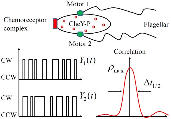
A central question in systems biology is to understand how molecular-level stimuli are converted into cellular behavioral responses. The signaling pathway and motor machinery in bacterial chemotaxis has been a prototypical system for us to gain insights into this question [1–14]. The chemotactic behavior of Escherichia coli follows a run-and-tumble pattern coordinated by multiple flagellar motors. Each motor spins either counterclockwise (CCW) or clockwise (CW), depending on the level of an intracellular response regulator, CheY-P, a phosphorylated form of CheY. Encountering attractant, the bacterial chemoreceptor complex rapidly pushes down the level of CheY-P, facilitating the CCW rotation of motors and the formation of a flagellar bundle that promotes the run movements. CW rotation of one or more motors disrupts the flagellar bundle and increases the frequency of tumble that reorients the cell. Slow adaptation of the system, achieved by a methylation and demethylation cycle, restores the chemoreceptor activity to a pre-stimulus level. As a result, the concentration of CheY-P fluctuates slowly with a characteristic time τx ~10–30s as determined by the slow time-scale of methylation kinetics [4, 11, 12]. Since motors in a single E. coli cell sense the same CheY-P signal (Fig. 1), a natural speculation arises: do different motors coordinate their switchings?
FIG. 1.
Two flagellar motors are regulated by a common CheY-P signal in an E. coli. Their output time traces, Y1(t) and Y2(t), are found to be highly correlated [17].
Biologists have probed this question decades ago and documented little evidence of correlation between rotatory motors in elongated mutant cells [15, 16]. Recent high-resolution measurements in wild-type (regular sized) cells [17], however, report a sharp correlation in motor switching, with a maximum correlation of ρmax ~ 0.5 and a half-width of Δt1/2 ~ 0.5s. The half-width Δt1/2 is defined as the full duration of time lag at half maximum (i.e., ρmax/2). How can such motor coordination be achieved? A plausible qualitative explanation [17] is that different motors, which are ultrasensitive to CheY-P levels [3], experience the same CheY-P fluctuations (Fig. 1). Here, we perform a detailed quantitative analysis of this novel phenomenon, using both theoretical and computational techniques. Our results demonstrate that the extrinsic CheY-P noise cannot account for the observed statistical features. Instead, we propose an intrinsic coupling model which is able to reproduce the sharp correlation profile. Our analysis suggests that there may be some direct interaction to coordinate the switching of motors. Possible coupling mechanisms and experimental proposals are suggested for future studies.
We first introduce and study a general model for the extrinsic mechanism of noise-induced correlation. Two motors in a single cell are regulated by a common input signal (e.g., CheY-P), denoted by X(t). The input is subject to the competitive effects of activation and deactivation, which make it fluctuate around an equilibrium level. Following [11], we describe the dynamics of X(t) by a Langevin equation:
| (1) |
where τx sets the input relaxation time and c represents the average input concentration. The stochastic term η(X, t) has zero mean 〈η(X, t)〉 = 0. To prevent X(t) from being negative, a multiplicative noise is used with the delta-correlation in time [18]: 〈η(X, t)η(X′, t′)〉 = σ2X(t)δ(t − t′). In steady state, X(t) follows a Gamma distribution with the variance . Thus, the relative noise level is , which is tunable by changing σ. In alignment with experimental data [3–6], the switching rates of each motor are taken to be for CCW-to-CW transitions and for CW-to-CCW transitions, where B(X(t)) is the probability of CW rotations (namely, the CW bias) depending on the current input level X(t) and where τy is the characteristic time of motor switching. According to the recent data for E. coli [3], the CW bias can be described by a Hill function: , with a response threshold Kd ≈ 3.1μM and a Hill coefficient h ≈ 10.3. Also, measurements indicate that τy ≈ 0.26s for E. coli [3–6].
Given the above specification, we can generate binary time traces of the two motors, Y1(t) and Y2(t), driven by the same input process X(t). Let Y1,2(t) = 0 denote the CCW rotation and Y1,2(t) = 1 the CW state. One can calculate their normalized cross-correlation [17]:
| (2) |
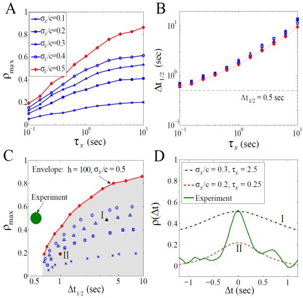
which peaks at zero time-lag (Δt = 0), as the two motors are assumed to observe the input signal simultaneously. This assumption can be justified by the fast diffusion of CheY-P or by applying to the case where the motors are equally close to the receptor source. Intuitively, we expect that the maximum correlation, ρmax ≡ ρ(0), increases with the input noise level ρx/c (Fig. 2A and Ref. [9]) and the motor's sensitivity h (data not shown). From Fig. 2A, the peak correlation becomes greater than 0.5 when τx > 1s and σx/c > 30%. The population-averaged estimate of CheY-P fluctuations is, however, less than 10% [7, 12], though one may argue that signaling noise in individual cells might be higher.
FIG. 2.
(color online). Simulation results for the extrinsic mechanism at c = Kd: (A) ρmax versus τx at different noise levels. The Hill coefficient, h, equals 10.3 for blue symbols and 100 for red symbols. (B) Δt1/2 versus τx for different noise levels. The symbols correspond to those in (A) based on the same simulations. (C) ρtmax and Δt1/2 derived from (A) and (B). The green spot represents the experimental observation which is out of the achievable region (shaded area) of the noise-induced model. (D) ρ(Δt) for the two representative points (I and II) in (C); each is obtained from 20-min simulated traces. The solid line denotes the correlation curve obtained from the 1-min experimental traces [17]; for better comparison, it is shifted to give a 0s-peak in correlation.
The major contradiction with experiments for this noise-induced mechanism is the mismatch of time scales, as illustrated in Fig. 2B. Irrespective of the noise level σx/c or the motor's sensitivity h, we find that Δt1/2 scales almost uniquely with the input characteristic time τx. This is because both motors are affected by the same CheY-P noise which has a much longer time scale [11]. We plot in Fig. 2C the phase space of ρmax and Δt1/2 by exhaustively searching the parameter space (h, σx/c, and τx) for this noise-driven model. The experimental observation (ρmax ~ 0.5 and Δt1/2 ~ 0.5s) is clearly out of the model's achievable region (shaded area in Fig. 2C, with the “envelope” corresponding to the extreme scenario: h = 100 and σx/c = 50%). As shown in Fig. 2D, the simulated ρ(Δt) cannot account for the experimental observation. Different forms of the noise term in Eq. (1) as well as different dependence of k± on X have been used in the model, all unable to explain the observed sharp correlation profile [19].
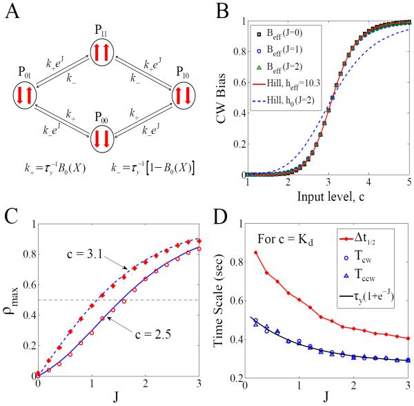
This puzzle inspires us to consider other mechanisms. We propose a testable hypothesis that the motors in question are directly coupled. Similar to the interaction in the Ising model [10, 14, 20], this intrinsic coupling makes the motors prefer being in the same state (which has a lower free energy). The idea is implemented by assuming the following instantaneous switching rates (Fig. 3A):
| (3) |
| (4) |
where is the CW bias of an individual motor (if without any coupling) and J ≥ 0 is the coupling strength in units of kBT. Generally, the joint process Y(t) = {Y1(t), Y2(t)} is non-Markovian due to the input stochasticity [18, 21]. However, if we mute the noise by setting X(t) = c, then Y(t) becomes a four-state Markov process which is analytically tractable. In this case, the effective CW bias of each motor is given by
| (5) |
where we find the apparent Hill coefficient for each motor is heff ≡ 2h0/(1 + e−J). Therefore, one can choose h0(J) = heff (1 + e−J)/2 such that the apparent CW bias is almost identical for any given value of J (Fig. 3B). Since Beff = 〈Y1,2(t)〉 and 〈Y1(t)Y2(t)〉 are both tractable, the maximum correlation, by Eq. (2), is found to be
| (6) |
This satisfies ρmax(c, J) ≤ ρmax(Kd, J) = tanh(J/2). We can get ρmax > 0.5 for moderate values of J (Fig. 3C).
FIG. 3.
(color online). Simulation results for the intrinsic mechanism under a constant input X(t) = c: (A) Illustration of the intrinsic coupling model. (B) Beff versus c by Eq. (5) for J = 0, 1, 2 and h0(J) = heff (1 + e−J)/2. The red line is the Hill function with heff = 10.3, while the blue line is the Hill function with a coefficient h0(J = 2). (C) ρmax versus J. Symbols are simulation results, compared to the theory (blue lines) by Eq. (6). (D) Δt1/2, Tcw, and Tccw versus J.
Now we examine the relevant time scales of motors under this constant input model. Using detailed balance, one can define the effective switching rates in equilibrium:
| (7) |
| (8) |
where , , and Pij denotes the equilibrium probability to find Y1 = i and Y2 = j. Since P01 = P10 by symmetry, calculating either of them will give us the analytical expressions of and . The inverses of these rates then tell us the average CCW and CW durations, which are found to be
| (9) |
| (10) |
For c = Kd, we have Tccw = Tcw = τy(1 + e−J). With the effective switching rates, we can also calculate the autocorrelation time, , of the output traces Y1,2(t) which exhibit an exponential autocorrelation function. Again, at c = Kd, this is simply , which decreases from τy to τy/2 as J increases from 0 to ∞. Note that the half-width Δt1/2 and the average (CW or CCW) durations are of the same order of magnitude (Fig. 3D). In other words, we have Δt1/2 ~ τy, consistent with the insight that the cross-correlation function will converge to the autocorrelation function when ρmax → 1. Clearly, the relation of Δt1/2 ~ τy < 1s under the intrinsic coupling mechanism (Fig. 3D) is distinct from that of Δt1/2 ~ τx > 1s under the extrinsic mechanism. So the intrinsic scheme seems to provide a plausible solution to the time-scale puzzle.
Though the constant input model is analytically convenient, we still need to investigate how the extrinsic noise and the intrinsic coupling intertwine together to affect the output statistics. This task relies on extensive Monte Carlo simulations for a mixture of the extrinsic and intrinsic mechanisms. To compare with the data, we choose parameter values that are experimentally relevant to E. coli: τx = 10s, c = 2.5νM, Kd = 3.1μM, σx/c ≤ 20%, and τy = 0.26s. The apparent Hill coefficient is also constrained by experiments [3], heff ≃ 10.3. This can be achieved by setting h0 = heff (1 + e−J)/2 for any given value of J. For c = 2.5μM and heff ≃ 10.3, the apparent CW bias in our model is 10–20%, consistent with the wild-type measurements [17]. Thus, J is the only free parameter remained in this setup.
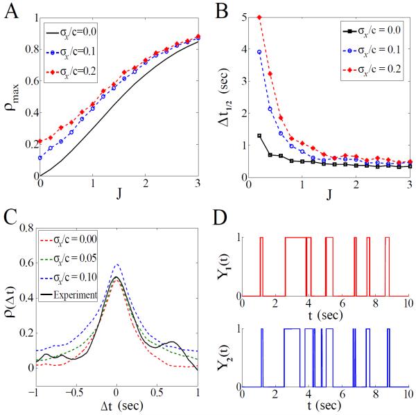
We plot ρmax and Δt1/2 versus J in Fig. 4A and 4B, respectively, which indicate that the intrinsic mechanism plays a dominant role when J > 1. A moderate coupling strength (J ~ 1.5) is sufficient to produce both ρmax ~ 0.5 and Δt1/2 ~ 0.5s, even in the presence of a weak noise σx/c < 10%. Indeed, the simulation result for J = 1.5 and σx/c = 5% provides a cross-correlation profile that closely resembles the experimental observation. Again, a comparison of ρ(Δt) at different noise levels (Fig. 4C) confirms that the intrinsic coupling makes the major contribution to the sharp correlation, while the extrinsic CheY-P variation adds only a small amount at large time scale. The high correlation is also evident when comparing the simulated motor traces (Fig. 4D).
FIG. 4.
(color online). Simulation results for the mixed mechanism at c = 2.5μM: (A) ρmax versus J for different noise levels. (B) Δt1/2 versus J. (C) ρ(Δt) for different noise levels with J = 1.5; each dashed line is obtained from 10-min simulated traces. The black solid line denotes the experimental correlation curve obtained from the 1-min traces in Ref. [17]. (D) Simulated time traces of the two motors.
All the results we presented imply that the temporal changes of CheY-P are not sufficient to explain the sharpness of correlation between motors in a single E. coli. There may be some other physical or biochemical process responsible for this observation. In [17], the authors have investigated the motor correlation in cells expressing a constitutively active CheY mutant, caCheY, which mimics the regulatory function (controlling CW rotations) of CheY-P. No significant correlation was detected in this mutant, suggesting that the motor coordination may require native CheY-P. However, the CW biases of motors in the same mutant cell are quite different as shown in the data [17]. This difference seems counterintuitive and may explain the disappearance of motor correlation [22]. The authors also made correlation analysis in cheZ (the gene encoding CheZ) deletion mutants where they found no coordinated switching either. Since CheZ is the phosphatase for CheY-P, removal of CheZ leads to saturating levels of CheY-P and hence very high CW bias. This could also suppress the motor correlation.
A time delay δt(< 0.2s) in the peak correlation was also reported in [17] and δt seems to increase with the distance between motors. It was argued that δt value may reflect the time required for CheY-P molecules to diffuse from the chemoreceptor patch to each motor. However, this explanation of finite δt depends on a wave-like propagation of CheY-P fluctuation in the cytosol and the source of CheY-P at only one pole of the cell; both of these assumptions may be questionable. In our model, we also observed a time delay in the peak correlation when the extrinsic effect of CheY-P noise dominates (small J and large σx/c) and when one motor senses the same but time-delayed input. However, we found no significant time shift in the peak when the intrinsic coupling effect dominates. This is due to the symmetric coupling between the two motors used in our current model. Breaking this symmetry in the model, e.g., by setting with J1 ≠ J2, can lead to an appreciable δt (depending on the degree of the asymmetry), even without a delay in CheY-P signal. This asymmetry in coupling may be caused by the internal asymmetry between the CW and CCW states [23] and by the external physical differences (different loads and different positions of the motors relative to the cell poles and the tethering substrate). The origin and the consequences of this asymmetry need to be fully explored in future studies.
What may cause the motor-motor coupling? Recent experiments show that bacterial motors respond not only to chemical cues (CheY-P) but also to mechanical signals (varying motor loads) [24, 25]. We speculate that a possible mechanism for the intrinsic coupling may be the hydrodynamic interaction between the rotating beads attached to the motors. Hydrodynamic synchronization has been experimentally reported in various physical and biological systems (e.g., the synchronous beating of eukaryotic cilia and flagella) [26]. Recent theoretical studies also shed light on hydrodynamic coupling in life at low Reynolds number [27–29]. Given the close distance between the motors in [17], we estimate that the effective load of one motor may change by ~ 30% when the other motor reverses its rotational direction [29, 30]. This (transient) change is not negligible and may cause a transient increase in the switching rates [13, 25]. According to the measurements in [25], we estimate that a 30% load change could contribute ~ 1kBT to the average amount of work performed by the stator on the rotor to promote switching [31]. This value is encouraging for the intrinsic mechanism, though a detailed model is needed to establish the connection. Hydrodynamic coupling is highly sensitive to the distance (l) between motors, since it decays as 1/l3 [29, 30]. Indeed, correlation was not detected between those motors separated by distances beyond 2.2μm in an elongated filamentous cell [17].
For the hypothesis of hydrodynamic coupling, we propose the following experimental test: repeat the experiment in [17] for a few minutes and then increase the viscosity of the medium (e.g., by adding Ficoll [25]) and continue the same measurement for another few minutes. If hydrodynamic coupling plays a role, we expect an even shaper correlation profile in the more viscous medium.
Acknowledgments
We are grateful to H. Fukuoka and A. Ishijima for providing us with their published data [17]. We thank H.C. Berg for bringing Ref. [29] to our attention. This research is supported by the NIH Grant GM081747.
References
- [1].Berg HC. Random Walks in Biology. Princeton, New Jersey: 1993. [Google Scholar]
- [2].Sourjik V, Berg HC. Nature. 2004;428:437. doi: 10.1038/nature02406. [DOI] [PubMed] [Google Scholar]
- [3].Cluzel P, Surette M, Leibler S. Science. 2000;287:1652. doi: 10.1126/science.287.5458.1652. [DOI] [PubMed] [Google Scholar]
- [4].Korobkova EA, et al. Nature. 2004;428:574. doi: 10.1038/nature02404. [DOI] [PubMed] [Google Scholar]
- [5].Korobkova EA, et al. Phys. Rev. Lett. 2006;96:058105. doi: 10.1103/PhysRevLett.96.058105. [DOI] [PubMed] [Google Scholar]
- [6].Park H, et al. Biophys. J. 2011;101:2336. doi: 10.1016/j.bpj.2011.09.040. [DOI] [PMC free article] [PubMed] [Google Scholar]
- [7].Park H, et al. Nature. 2010;468:819. doi: 10.1038/nature09551. [DOI] [PMC free article] [PubMed] [Google Scholar]
- [8].Emonet T, Cluzel P. Proc. Natl. Acad. Sci. U.S.A. 2008;105:3304. doi: 10.1073/pnas.0705463105. [DOI] [PMC free article] [PubMed] [Google Scholar]
- [9].Sneddon MW, Pontius W, Emonet T. Proc. Natl. Acad. Sci. U.S.A. 2012;109:805. doi: 10.1073/pnas.1113706109. [DOI] [PMC free article] [PubMed] [Google Scholar]
- [10].Mello BA, Tu Y. Proc. Natl. Acad. Sci. U.S.A. 2003;100:8223. doi: 10.1073/pnas.1330839100. [DOI] [PMC free article] [PubMed] [Google Scholar]; ibid. 2005;102:17354. [Google Scholar]
- [11].Tu Y, Grinstein G. Phys. Rev. Lett. 2005;94:208101. doi: 10.1103/PhysRevLett.94.208101. [DOI] [PubMed] [Google Scholar]
- [12].Shimizu TS, Tu Y, Berg HC. Mol. Syst. Biol. 2010;6:382. doi: 10.1038/msb.2010.37. [DOI] [PMC free article] [PubMed] [Google Scholar]
- [13].van Albada SB, Tanase-Nicola S, ten Wolde PR. Mol. Syst. Biol. 2009;5:316. doi: 10.1038/msb.2009.74. [DOI] [PMC free article] [PubMed] [Google Scholar]
- [14].Endres RG, Wingreen NS. Proc. Natl. Acad. Sci. U.S.A. 2006;103:13040. doi: 10.1073/pnas.0603101103. [DOI] [PMC free article] [PubMed] [Google Scholar]
- [15].Macnab RM, Han DP. Cell. 1983;32:109. doi: 10.1016/0092-8674(83)90501-9. [DOI] [PubMed] [Google Scholar]
- [16].Ishihara A, et al. J. Bacteriol. 1983;155:228. doi: 10.1128/jb.155.1.228-237.1983. [DOI] [PMC free article] [PubMed] [Google Scholar]
- [17].Terasawa S, et al. Biophys. J. 2011;100:2193. doi: 10.1016/j.bpj.2011.03.030. [DOI] [PMC free article] [PubMed] [Google Scholar]
- [18].Hu B, et al. Phys. Rev. E. 2012;86:061910. doi: 10.1103/PhysRevE.86.061910. [DOI] [PMC free article] [PubMed] [Google Scholar]
- [19].For example, we can also model the CheY-P signal as an Ornstein-Uhlenbeck process or a Poisson process, or assume that τy in the transition rates k+ and k− is a function of X (by setting τy(X) = τ0(1 + X/c)/2 for example). Such model variants, however, cannot generate the observed sharp correlation profile.
- [20].Hu B, et al. Phys. Rev. Lett. 2010;105:048104. doi: 10.1103/PhysRevLett.105.048104. [DOI] [PMC free article] [PubMed] [Google Scholar]; Hu B, et al. Phys. Rev. E. 2011;83:021917. doi: 10.1103/PhysRevE.83.021917. [DOI] [PMC free article] [PubMed] [Google Scholar]
- [21].Hu B, et al. Phys. Rev. Lett. 2011;107:148101. doi: 10.1103/PhysRevLett.107.148101. [DOI] [PMC free article] [PubMed] [Google Scholar]
- [22].Fukuoka H, Ishijima A. private communication. [Google Scholar]
- [23].Yuan J, et al. Proc. Natl. Acad. Sci. U.S.A. 2010;107:12846. doi: 10.1073/pnas.1007333107. [DOI] [PMC free article] [PubMed] [Google Scholar]
- [24].Fahrner KA, Ryu WS, Berg HC. Nature. 2003;423:938. doi: 10.1038/423938a. [DOI] [PubMed] [Google Scholar]
- [25].Yuan J, Fahrner KA, Berg HC. J. Mol. Biol. 2009;390:394. doi: 10.1016/j.jmb.2009.05.039. [DOI] [PMC free article] [PubMed] [Google Scholar]
- [26].Meiners JC, Quake SR. Phys. Rev. Lett. 1999;82:2211. doi: 10.1103/PhysRevLett.84.5014. [DOI] [PubMed] [Google Scholar]; Kim MJ, et al. Proc. Natl. Acad. Sci. U.S.A. 2003;100:15481. [Google Scholar]; Riedel IH, Kruse K, Howard J. Science. 2005;309:300. doi: 10.1126/science.1110329. [DOI] [PubMed] [Google Scholar]; Kotar J, et al. Proc. Natl. Acad. Sci. U.S.A. 2010;107:7669. doi: 10.1073/pnas.0912455107. [DOI] [PMC free article] [PubMed] [Google Scholar]; Polin M, et al. Science. 2009;325:487. doi: 10.1126/science.1172667. [DOI] [PubMed] [Google Scholar]; Goldstein RE, Polin M, Tuval I. Phys. Rev. Lett. 2009;103:168103. doi: 10.1103/PhysRevLett.103.168103. [DOI] [PubMed] [Google Scholar]
- [27].Vilfan A, Jülicher F. Phys. Rev. Lett. 2006;96:058102. doi: 10.1103/PhysRevLett.96.058102. [DOI] [PubMed] [Google Scholar]
- [28].Ryskin A, Lenz P. Phys. Biol. 2006;3:285. doi: 10.1088/1478-3975/3/4/006. [DOI] [PubMed] [Google Scholar]
- [29].Uchida N, Golestanian R. Phys. Rev. Lett. 2011;106:058104. doi: 10.1103/PhysRevLett.106.058104. [DOI] [PubMed] [Google Scholar]
- [30].The load contribution by hydrodyamic interaction is estimated by the geometric factor 9ah2/l3 derived in [29], where a ~ 0.25μm is the bead radius, h ~ 0.μm is the height of the bead to the substrate, and l ~ 1.5μm is the typical distance between motors. When one motor reverses its rotational direction, its e ecitve drag on the other motor is changed by a factor of 2. Thus, the effective load change due to hydrodynamic interaction is estimated to be 18ah2/l3 ≈ 33%.
- [31].A CCW rotation speed of 150Hz corresponds to a torque of Γ ~ 103pN · nm according to [25]. A 30% change in the torque amounts to a change of 0.3 · Γ · θ ≈ 1kBT in the free energy barrier between the CW and CCW states, where θ ≈ 3.3 × 10⁻³kBT/(pN · nm) as estimated in [25].


