A Hybrid Least Squares and Principal Component Analysis Algorithm for Raman Spectroscopy

Abstract

The least squares fitting algorithm is the most commonly used algorithm in Raman spectroscopy. In this paper, however, we show that it is sensitive to variations in the background signal when the signal of interest is weak. To address this problem, we propose a novel algorithm to analyze measured spectra in Raman spectroscopy. The method is a hybrid least squares and principal component analysis algorithm. It explicitly accounts for any variations expected in the reference spectra used in the signal decomposition. We compare the novel algorithm to the least squares method with a low-order polynomial residual model, and demonstrate the novel algorithm’s superior performance by comparing quantitative error metrics. Our experiments use both simulated data and data acquired from an in vitro solution of Raman-enhanced gold nanoparticles.

I. INTRODUCTION

Raman spectroscopy is a powerful technique for analyzing chemical compounds using laser light. It works by exploiting the Raman effect, which is explained as follows. When incoming photons hit a sample surface, most photons are scattered elastically, after which they continue traveling with the same energy and wavelength. However, a very small fraction of the photons is scattered inelastically, meaning that they lose energy and continue traveling with a longer wavelength. The amount of energy lost by the photons depends on the particular molecules they interact with. In fact, the chemical bonds in the molecules absorb energy in highly specific patterns. As a result, the Raman scattered photons possess highly compound-specific wavelength spectra.

Raman spectroscopy exploits the Raman effect in order to identify and quantify compound concentrations. It does so by exciting a particular sample with photons from a laser beam, and measuring the highly specific spectral fingerprints of the resulting Raman scattered photons. Given that they are known a priori, the spectra of compounds of interest can then be extracted from the measured spectrum using an appropriate signal analysis algorithm. Raman spectroscopy allows rapid sample analysis of single or multiple compounds (known as multiplexed analysis) at high detection sensitivities [5]. Amongst its many promising areas of application, Raman spectroscopy has gained overwhelming interest from the biomedical research community, where it promises to enable sensitive imaging of nanoparticles for both diagnostic and therapeutic applications [1], [5].

Various methods have been used to analyze Raman spectra (i.e. detect and potentially quantify compounds), such as ordinary least squares [5], least squares with a low-order polynomial background model [3], and principal component analysis [4], [2]. While fast and quantitative, the ordinary least squares method is sensitive to variations in the background spectrum and known compound spectra supplied to the algorithm. Lutz et. al [3] addressed this problem by allowing the background spectrum to vary according to a low-order polynomial model. While this reduces the sensitivity of the least squares fit to variations in the background signal, the algorithm cannot accommodate higher-order variations such as the slight peak shifts and changes in the relative amplitudes of peaks that have been observed in practice. The principal component analysis (PCA) method is a non-parametric method that does not require an explicit background model. However, while useful as a classification method for determining whether or not a particular compound is present, PCA does not explicitly quantify the signal strength of any compounds present.

In the current work, we develop a novel algorithm that combines the strengths of least squares algorithms (quantitative) and PCA methods (non-parametric). We test it on both simulated data and data acquired from an in vitro solution of Raman-enhanced gold nanoparticles [5]. From here on, we refer to our method as the hybrid least squares and principal component analysis (HLP) algorithm. Section II presents the mathematical details of the method. Section III demonstrates the improved performance of the novel method compared to that of the least squares method with an explicit background model [3].

II. METHODS

A. Least squares method with explicit background model

Here we briefly review the least squares method with a low-order polynomial residual model, as proposed by Lutz. et al. [3]. The measured spectrum can be modeled as a linear combination of known spectra (a.k.a. reference spectra):

$$x_l=\sum _{k=1}^K{w}_k{S}_{lk},w_k\ge 0,$$ (1)

where x_l is the modeled intensity at wavelength l, K is the number of reference spectra provided, S_lk is the value of the reference spectrum of the k^th compound at wavelength l, and w_k is the weight for the k^th compound. In the method proposed by Lutz et al. [3], the spectra S_k include the compounds of interest as well as an average background signal and the q + 1 components of a q^th order polynomial. The concentrations of the various compounds are then estimated by solving for the weights w_k that give the closest fit with the measured spectrum. This can be done by writing the problem in the matrix form M = SW, where M is the L×1 vector containing the measured spectrum values m_l, S is the L×K matrix of reference spectra, and W is the K ×1 matrix containing the weights w_k. The least squares solution is then given by Ŵ = S^†M, where S^† = (S^T S)⁻¹ S^T is the Moore-Penrose pseudoinverse of the matrix S.

B. Novel hybrid algorithm (HLP)

As mentioned, the low-order polynomial model used above cannot account for higher-order variations such as changes in peak position and relative amplitude. Here we extend the signal model in order to account for such variations. More specifically, we allow each of the reference spectra S_k (not including low-order polynomial terms) to vary according to the principal components of variation observed in sets of previous scans of the respective compounds in isolation¹. For each reference spectrum, we penalize deviations from the mean signal in accordance with the eigenvalues obtained from the principal component analysis. In essence, this constrains the variations in the reference spectra to the statistically plausible. Mathematically, we extend the signal model to

$$x_l=\sum _{k=1}^K{w}_k\left({\overline{S}}_{lk}+\sum _{p=1}^P{c}_{pk}{Z}_{\mathit{lpk}}\right),$$ (2)

where S̄_k is the mean spectrum observed for compound k, and Z_pk is the p^th principal component with a non-zero eigenvalue for compound k, observed during prior characterization experiments. Our objective is now to estimate the coefficients W = {w_k} and C = {c_pk} that give the best signal fit. We do so by using a Bayesian probability framework, where we maximize the posterior probability of W and C, given the measured signal M, the mean reference spectra S̄, the principal components Z, and the eigenvalues λ (corresponding to Z). Using Bayes’ theorem and the rules of conditional probability, we can decompose this posterior probability as

$$P(W,C\mid M,\overline{S},Z,\lambda )=P(M\mid \overline{S},Z,W,C)P(C\mid \lambda )P(\lambda )P(\overline{S})P(Z)P(W)\frac{1}{\mathcal{N}},$$ (3)

where is a normalization constant, and we recognized that P (M|S̄, Z, λ, W, C) = P (M|S̄, Z, W, C). We also assumed S̄, Z, W, and C are statistically independent of each other.

The first term of Eqn. 3 is the data likelihood term. Assuming statistical independence of the samples at each wavelength, it is given by

$$P(M\mid \overline{S},Z,W,C)=\prod _{l=1}^{L}P(m_l\mid \overline{S},Z,W,C).$$ (4)

Assuming a zero-mean Gaussian noise model, the probabilities P (m_l|S̄, Z, W, C) are given by

$$P(m_l\mid \overline{S},Z,W,C)=\frac{1}{\sqrt{2\pi }\sigma }{e}^{-\frac{{(m_l-x_l)}^2}{2{\sigma }^2}},$$ (5)

where σ is the standard deviation of the noise in the measured signal. It can be estimated by taking repeated measurements of the same location on a given sample. For the second term in Eqn. 3, we assume that the coefficients c_pk are independent, which yields

$$P(C\mid \lambda )=\prod _{k=1}^K\prod _{p=1}^{P}P(c_{pk}\mid \lambda ),$$ (6)

where P is the number of non-zero eigenvalues². By definition, the eigenvalues λ_pk obtained by the principal component analysis are equal to the variance of the coordinates obtained when projecting all data points on the principal component axis corresponding to λ_pk, i.e. ${\lambda }_{pk}={\sigma }_{pk}^2$. Hence we have

$$P(c_{pk}\mid \lambda )=\frac{1}{\sqrt{2\pi }\sigma }{e}^{-\frac{c_{pk}^2}{2{\sigma }_{pk}^2}}.$$ (7)

Next, the prior probabilities P (λ), P (S̄), and P (Z) are independent of W and C, and are hence of no consequence to our optimization problem. Lastly, we assume a uniform distribution for P (W).

Following standard practice in optimization problems, we optimize the logarithm of the Bayesian cost function given in Eqn. 3. This simplifies the optimization problem by converting multiplications into summations. After dropping constant terms and cancelling common factors, the cost function can be reduced to

$$\psi (W,C)=-\sum _{l=1}^L{(m_l-x_l)}^2-\beta \sum _{k=1}^K\sum _{p=1}^P\frac{c_{pk}^2}{{\sigma }_{pk}^2}$$ (8)

where β = σ². Note that Eqn. 8 takes the familiar form of a penalized maximum likelihood (PML) problem, where β functions as the hyperparameter.

The cost function in Eqn. 8 can be efficiently optimized (maximized) by alternatingly solving it as a standard least squares problem in W, and a Tikhonov regularized least squares problem in C. Convergence was observed in all experiments after on the order of 100 iterations. For the experiments in Section III, where L = 1015, the time per iteration was 0.02 seconds. All coefficients were initialized with a zero initial guess. The expression for the update of the coefficients w_k is, similar to in Section II-A, given by Ŵⁿ = S^†nM, where S^†n is the Moore-Penrose pseudoinverse of the n^th estimate of the L × K matrix S, which is composed of the signals $S_{lk}={\overline{S}}_{lk}+{\sum }_{p=1}^P{c}_{pk}^n{Z}_{\mathit{lpk}}$, where $c_{pk}^n$ are the latest estimates of c_pk. To obtain the update steps for the coefficients c_pk, it is instructive to substitute Eqn. 2 into Eqn. 8, and to rewrite the latter as

$$\psi (C)=-\sum _{l=1}^L{\left(p_l-\sum _{k=1}^K\sum _{p=1}^P{c}_{pk}{w}_k^n{Z}_{\mathit{lpk}}\right)}^2-\beta \sum _{k=1}^K\sum _{p=1}^P\frac{c_{pk}^2}{{\sigma }_{pk}^2},$$ (9)

where $p_l=m_l-{\sum }_{k=1}^K{w}_k^n{\overline{S}}_{lk}$, and $w_k^n$ are the latest estimates of w_k. To formulate our update step, we store the elements p_l into an L×1 vector Q, and the elements $w_k^n{Z}_{\mathit{lpk}}$ in an L×KP matrix A = {w_kZ_lpk}. The matrix C is of size KP ×1. Maximizing Eqn. 9 is then equivalent to minimizing the cost function

$$\varphi (C)=-\psi (C)={\Vert AC-Q\Vert }^2+{\Vert \mathrm{\Gamma }C\Vert }^2,$$ (10)

where $\mathrm{\Gamma }=\sqrt{\beta }{I}_{{\sigma }^{\prime }}$, and I_σ′ is a KP × KP diagonal matrix that contains the values $\frac{1}{{\sigma }_{pk}}=\frac{1}{\sqrt{{\lambda }_{pk}}}$ along its diagonal entries. Eqn. 10 is a standard Tikhonov regularized least squares problem, and has the explicit solution

$$\widehat{C}={(A^{T}A+{\mathrm{\Gamma }}^T\mathrm{\Gamma })}^{-1}{A}^{T}Q.$$ (11)

III. RESULTS

Here we compare the performance of the least squares algorithm using a third-order polynomial background model (LS-3P)³ to that of our hybrid least squares PCA (HLP) algorithm, for various nanoparticle signal strengths (see below). We present preliminary results for cases where K = 2. In other words, the signals considered contain one compound spectrum of interest and one significant background signal.

A. Simulation results

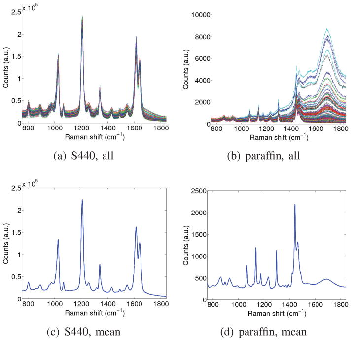
In this section, we simulated the presence of a signal of interest within a background signal. Both signals were subject to a realistic amount of variability. The experiment was repeated for various relative amplitudes of the signal of interest, and was designed to characterize the accuracy with which the weight of the signal of interest could be recovered, in spite of variability in both the signal of interest and the background signal. To obtain a realistic amount of signal variability, we collected real Raman spectroscopy signals from a 0.8nM solution of Raman-enhanced S440 gold nanoparticles produced by Oxonica (now owned by Cabot Security Systems, Boston, MA, USA), as well as signals from a paraffin background material. By performing raster scans across the solution as well as background material, we obtained 106 signals for the S440 nanoparticle solution, and 476 signals for the paraffin background. The collection of all signals and the mean signal for each set are shown in Fig. 1.

Fig. 1.

Acquired signals and mean signal. Left: S440 nanoparticle. Right: paraffin background.

For each simulated S440 signal strength, we performed a series of leave-one-out experiments. In each such experiment, we picked one S440 signal, and one paraffin background signal. The remaining signals in our data base were then used to compute the mean S440 and background signals, as well as their respective principal components. We then simulated a measurement signal by weighting the chosen S440 signal and adding it to the chosen paraffin background signal⁴. This was done for S440 weights of 2⁰, 2⁻¹, …, 2⁻¹², and 2⁻¹³.

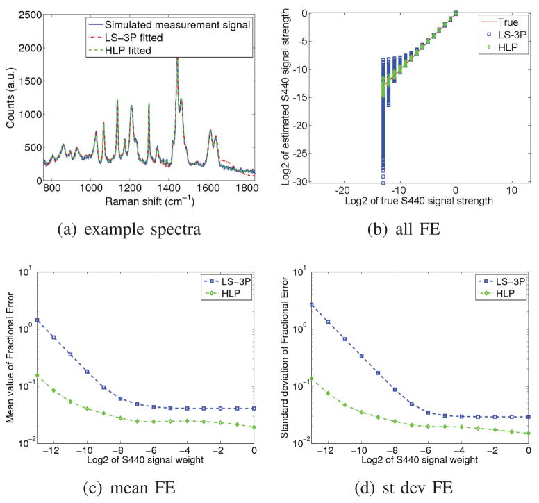
The performance of each method was evaluated using the fractional error, defined as $FE=\frac{\mid W_{\mathit{est}}-W_{\mathit{true}}\mid }{W_{\mathit{true}}}$, where W_est and W_true are the estimated and true weights of the S440 signal (which are roughly linearly related to the nanoparticle concentration). An example spectrum, as well as the fitted spectra by LS-3P and HLP are shown in Fig. 2(a). The fractional errors, as well as their mean and standard deviation are shown for both algorithms in Fig. 2(b–d). The HLP algorithm clearly outperforms the LS-3P algorithm at all weights/concentration levels for the S440 signal, and most markedly so at lower strengths of the S440 signal.

Fig. 2.

(a) Example of fitted spectra and (b–d) fractional errors by the LS-3P and HLP algorithms.

B. Experimental results

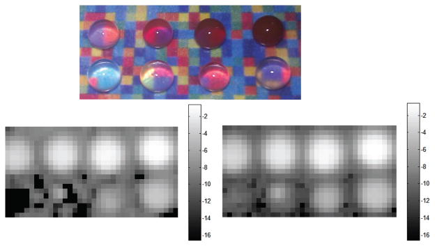
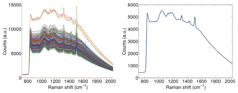
To demonstrate that HLP outperforms LS-3P on experimental data as well, we designed another example where the background signal varied significantly. We placed eight drops of decreasing concentrations of S440 nanoparticles on paraffin, which was in turn placed on a background of various colors (see Fig. 3). The colors each had distinct Raman spectra, and were obtained by printing a color image of a matrix of random numbers between 0 and 1. The mean signal, as well as the collection of all signals obtained from a raster scan of the background are shown in Fig. 4. The first drop had a concentration of 0.8nM, and subsequent drops were obtained by each time halving the concentration. The logarithm-transformed (base 2) images of the estimated S440 signal strength are shown in Fig. 3 for both the LS-3P and HLP algorithms. The black pixels in the images are points for which the algorithms produced negative weights. The signal estimates by HLP and LS-3P are almost identical when the nanoparticle signal strength is high. However, HLP proves far more stable than LS-3P when the nanoparticle signal strength is low (i.e. when variations in the background signal become more significant). The relationship between the drop concentrations and the estimated signal weights was found to be approximately linear (not shown due to space limitations).

Fig. 3.

Top: Experimental phantom. Middle: log2 of S440 signal by LS-3P. Bottom: log2 of S440 signal by HLP.

Fig. 4.

Signals from background scan. Left: all signals. Right: mean signal.

IV. CONCLUSIONS AND FURTHER WORK

A. Conclusions

In this work, we showed that the LS-3P algorithm for Raman spectroscopy is sensitive to variations in the background signal when the nanoparticle signal of interest is weak. We proposed a novel algorithm (HLP) that is more robust to such background variations. Improved performance was shown for both simulated and experimental data. The simulated data was generated by digitally combining weighted instances of experimentally obtained background and nanoparticle spectra. The experimental data was obtained from serially diluted in vitro solutions of Raman-enhanced gold nanoparticles.

B. Further work

While the background signal in our experimental data was of an artificial nature (obtained from a color printout from an office printer), we expect the HLP algorithm to become useful for future in vivo experiments, where inherent tissue variations or variations in ambient light may cause background signal variations. A likely example is joint white light and Raman colonoscopy, where both the tissue background and the intensity of the LED light reflecting from the colon wall may vary. The varying contributions of ambient light cannot be generally captured by a low-order polynomial. In our future work, we will also further characterize the quantitative accuracy of the HLP algorithm in terms of its ability to estimate the concentration of one or more nanoparticle solutions. Second, we will evaluate the merits of a Poisson instead of Gaussian noise model in decreasing the lowest detectable nanoparticle concentration. Third, we will examine the performance of HLP for multiplexed spectroscopy (K > 2). Lastly, we will evaluate the performance of HLP for in vivo imaging data (eg., in mice or in pig colon).

References

- 1.Fortina P, Kricka LJ, Surrey S, Grodzinski P. Nanobiotechnology: the promise and reality of new approaches to molecular recognition. TRENDS in Biotechnology. 2005;23(4):168–173. doi: 10.1016/j.tibtech.2005.02.007. [DOI] [PubMed] [Google Scholar]
- 2.Guicheteau J, Argue L, Emge D, Hyre A, Jacobson M, Christesen S. Bacillus Spore Classification via Surface-Enhanced Raman Spectroscopy and Principal Component Analysis. Applied spectroscopy. 2008;62(3):267–272. doi: 10.1366/000370208783759623. [DOI] [PubMed] [Google Scholar]
- 3.Lutz BR, Dentinger CE, Nguyen LN, Sun L, Zhang J, Allen AN, Chan S, Knudsen BS. Spectral analysis of multiplex Raman probe signatures. ACS nano. 2008;2(11):2306–2314. doi: 10.1021/nn800243g. [DOI] [PMC free article] [PubMed] [Google Scholar]
- 4.Ryder AG. Classification of narcotics in solid mixtures using principal component analysis and Raman spectroscopy. Journal of forensic sciences. 2002;47(2):275–284. [PubMed] [Google Scholar]
- 5.Zavaleta CL, Smith BR, Walton I, Doering W, Davis G, Shojaei B, Natan MJ, Gambhir SS. Multiplexed imaging of surface enhanced Raman scattering nanotags in living mice using noninvasive Raman spectroscopy. Proceedings of the National Academy of Sciences. 2009;106(32):13511. doi: 10.1073/pnas.0813327106. [DOI] [PMC free article] [PubMed] [Google Scholar]