Conservation Priorities when Species Interact: The Noah's Ark Metaphor Revisited

Abstract

This note incorporates ecological interactions into the Noah's Ark problem. In doing so, we arrive at a general model for ranking in situ conservation projects accounting for species interrelations and provide an operational cost-effectiveness method for the selection of best preserving diversity projects under a limited budget constraint.

Introduction

Weitzman [13] is a milestone in the economic theory of biodiversity. His “Noah's Ark Problem” is not only a modeled metaphor that is helpful to organize thinking on how to face conservation trade-offs with finite resources. It also results in a practical cost-effectiveness methodology that can serve as inspiration to guide conservation policies. The idea is, for each species , to collect information about: , the cost of its protection, the increase of survival probability resulting from it, , the direct utility of how much we value the species, its distinctiveness. From this information, each species is assigned a number via the formula:

(1)

which indicates its rank in conservation priorities. This ranking criterion has a theoretical foundation: it is rooted in a rigorous optimization model ([13], Theorem 4, p. 1295).

This criterion sheds light on real biodiversity issues and has actually been used in several applications. Some of these have led to changes in allocation of conservation funding (e.g., in New Zealand; [9]), and variants have been used to allocate surveillance effort over space (e.g., [8]). Other applications are quoted in [5]. But it is fair to say that this approach is more appropriate for ex situ conservation projects - say to build a gene bank or a zoo - rather than to manage a set of interacting species in their natural habitats. This is so because formula (1) uses no information of any kind about the web of life. Yet, in ecosystems, species interact. Some of them compete to share common resources, others develop synergies and mutually enhance each other or they simply pertain to the same trophic chain. Suppose, then, that the conservation authority has information about those ecological interactions, even if it is only under the rudimentary form of survival probability interdependencies. That is, it knows that a marginal increase of survival probability of species will have an impact on the survival probability of species . Could this information be used to qualify formula (1) and increase its relevance when it comes to in situ conservation trade-offs?

To our knowledge, three recent articles stress the need to account for ecological interactions in Weitzman's diversity concept. They have in common: to take into account the ecological interactions via interdependent survival probabilities in a simplified version of the Noah's Ark metaphor with two species [1], [11] or three species [12], to show that this consideration can reverse the conservation priorities. The key of this note is to provide a general analysis of in situ conservation problems considering interdependent survival probabilities. Revisiting Weitzman's optimization problem, we extend his model in order to incorporate species interactions. Our principal output is to forward a general ranking formula that could be used as a rule of thumb for deciding in situ conservation priorities under a limited budget constraint.

The sketch of the paper is the following. Section 2 incorporates ecological interactions in Weitzman's parable of Noah's Ark, with any arbitrary number of species. The crux of the section is to provide with a new rule for establishing in situ conservation priorities through the expression (12) below that encompasses formula (1) as a special case. The link between this formula and Noah's optimal policy is explained. Section 3 illustrates the relevance of this new formula within a two-species example. We check the robustness of our formula and end the paper with a discussion on the possibility of ranking reversal in relation to three stylized kinds of ecological interactions: predation, mutualism and competition.

Analysis

The “Noah's Ark Problem” is a parable intended to be a kind of canonical form representing how best to preserve biodiversity under a limited budget constraint. In the initial version of Weitzman's modeled allegory, Noah's decision problem is, for each species , to choose a survival probability between a lower and an upper bound, , in order to maximize the sum of the expected diversity function:

and the expected utility of the set of species:

Weitzman devotes much of his paper to defining the expected diversity function and to explaining its link with the concept of information content (see his Theorem 1, p. 1284). This function could take various specific forms, depending on the way dissimilarity is conceptualized. A precise example, from [13], is discussed in Section 4. In order for our results to remain as general as possible, we simply consider in this paper the class of functions, i.e whose first and second order derivative both exist and are continuous.

And we assume they admit Hessian matrices that are nowhere negative semi-definite, i.e there is no admissible such that the Hessian of is negative semi-definite at . Weitzman's expected diversity function belongs to this class. It encompasses - but is not limited to - functions with a positive definite Hessian matrix, i.e. that are strictly convex functions.

Now let us take a step away from this initial metaphor, towards reality. Two modifications are brought into the formalism. First, rather than controlling directly the probability of survival of each species Noah can exert a protection effort within an admissible range, which is interpreted as the controlled increase of survival probability - say that is the increase of survival probability for species resulting from a protection effort, e.g. an investment in a vaccination campaign, the provision of supplementary food, the protection and enhancement of habitat [6]. It is important to distinguish the effort from the change in the survival probability because is also determined by other factors, for there are ecological interactions among species. And this is where our second, most important, qualification appears: probabilities of survival are interdependent and the nature of those interactions are known. Nowadays, Noah can rely on the knowledge gained from the new and booming conservation biology literature on species distribution models and population viability analysis. See for instance[3], [14], [7], or [4] for a recent overview. Note that this literature does not take into account directly of species interactions; it just provides estimates of probabilities in space and time. From there, although applied econometric problems will have to be overcome, correlations between probabilities could be estimated.

A group of experts can measure the marginal impact, say , that an increase in the probability of survival of a species can have on the probability of survival of another species The experts can also appraise the impact of protection efforts on these probabilities. Assume, then, that the relationships between extinction risks are linear. Put differently, a tractable approximation of all those pieces of information can be summarized by the system (2) of linear equations:

(2)

There are biological and economic factors that determines eligible efforts. Formally, admissible ranges of efforts are Implicitly, additional efforts beyond the threshold have no effect on the survival probabilities. And we assume:

We denote as the survival probability of species without any conservation efforts, In the absence of natural interactions, which corresponds to the case studied by Weitzman, we have . A consequence is that in the very particular case with no ecological interactions and no conservation efforts, species has a probability of survival . The survival probabilities interval, without ecological interactions, would thus take values ranging from to

Noah also has to cope with a budget constraint:

(3)

where is the total budget to be allocated to conservation - metaphorically, the size of the Ark - and is the cost per unit of effort to preserve species .

It is worthwhile making three remarks about this budget constraint. Firstly, it is assumed that changes in extinction probability are a linear function of expenditure. This may be inconsistent in real world applications where the marginal expense needed to reduce extinction risks is increasing. For example, [10] documents that the marginal preservation cost of threatened Australian birds increases when probability of extinction approaches zero. Weitzman rightly defends this linearity assumption as an acceptable approximation when the variation of probability falls in a sufficiently narrow range. But clearly, if costs are non linear and convex functions of efforts, an important qualitative result of our paper could change (Theorem 1 below may not hold any longer). Secondly, as a formal matter one could retrieve Weitzman's model with a simple change of variable, where is the cost per unit of increase of survival probability in the range Thirdly, except when ecological interactions are negligible, Noah can increase the probability of survival of any species via two different channels: a direct one by increasing the protection effort at a cost and an indirect one through ecological interactions, due to the protection of another species , with a cost

Noah's Ark problem, when ecological interactions are taken into account, is then:

(4)

subject to (2) and (3).

It will be convenient subsequently to work with matrix or vector expressions, written in bold characters. For any matrix , let denote its transpose. Further, is the identity matrix, is the dimensional column vector whose elements are all 1, and we recall the following definition of inequality between two -dimensional vectors and with components and respectively: if for all The other basic relationships between vectors are: if for all if for all if for all and We also need basic matrix operations, “+”, “-” and “*”, that refer to, respectively the addition, the subtraction and the multiplication.

Let us define:

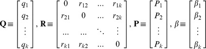In matrix form, the system (2) reads as:

(5)

Throughout this article, we will assume:

Assumption 1 (INV) The matrix is invertible.

Under Assumption (INV), the system (5) can be solved to give:

(6)

where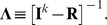

Let refer to the affine mapping from efforts to probabilities. Survival probabilities without protection policies are therefore:

(7)

where is a vector made of zeroes. Without ecological interactions, is the identity matrix, and

Now we can plug (6) into (4) to get rid of probabilities, and express Noah's problem only in terms of efforts. Define the two composite functions, which here are mappings from the values taken by function to the set of real numbers:

Under Assumption (INV), to each vector corresponds a unique vector . Therefore we can define Noah's problem with ecological interactions, the constrained maximization of a function of protection efforts :

(8)

subject to:

(9)

(10)

Results

Two questions arise: could anything general be said about the solution to the problem expressed by (8), (9), (10)? And , taking a more practical stance, could we engineer a simple rule that approximates the general solution?

Noah's policy is extreme

Weitzman [13] showed that the solution to Noah's problem lies on the boundary of the efforts set. As the set of constraints is made of linear constraints, the boundary involves corners, e.g. or and possibly a segment between two corners, therefore with for at most one species. This can be defined as an extreme policy. In words, the optimal protection policy gives full protection to a subset of species, partial protection for at most one species, and exposes the remaining species to the risk of no protection.

But what if probabilities are interdependent? We show that when species interact, the optimal solution is also extreme.

Theorem 1 The solution to Noah's Ark problem with ecological interactions, defined by (8), (9) and (10), is an extreme policy.

Proof

The proof rests on two pieces of information:

1. Noahs' problem is to maximize a continuous function over a compact set, therefore by Weiestrass extreme value theorem there exists a solution.

2. The Hessian matrix of is not negative semi-definite, a statement we shall prove below.

Item ii) violates the necessary second order condition for interior solutions to Noah's problem and, in combination with item i), leads to conclude the existence of a solution on the boundary of the efforts set.

In order to prove item ii), because is linear, we just have to ensure that the Hessian matrix of is not negative semi-definite. Recall that is a -dimensional vector with typical element , and let stand for the Jacobian matrix:

Note that, since each function is linear, the Jacobian matrix is made of invariant numbers, so we need not mention the application point and we can simply refer to the matrix .

Denote the Hessian matrix of a matrix with typical elements . From meticulous derivations of the composite function , and after simplifications allowed by the linearity of the mapping , one obtains:

If is negative semi-definite, then for any nonzero vector we must have:

Notice that is simply a nonzero vector, which we may simply call . Hence we can rewrite the above inequality as:

which would mean that is negative semi-definite, a possibility that has been ruled out by assumption. ▪

A ranking rule for interacting species

Theorem 1 is a qualitative result, that does not indicate which species should be granted protection and why. This brings us to our second question; it would be welcome to have an explicit and easy-to-use approximation of the general solution. Facing the same problem, this is the practical point of view adopted by [13], which he describes as “the main theme” of his paper (p. 1294). His formula (1) offers a ranking that is not really a solution to the original problem, but rather a first order approximation of an optimal policy. In order to achieve this, he replaces the objective function by its linear approximation. He then obtains a classical linear programming problem, whose solution is to assign grades given by formula (1) to species (those grades depend on the model parameters) and order them in decreasing order of importance up to the point where the budget is exhausted. Those grades are exactly the practical ranking Noah is looking for.

We follow the same approach here, i.e. we linearize the objective function. The astute reader knows that, in general, such approximations can be seriously misleading [2] and should not be followed blindly. Nevertheless, as proven in Theorem 2 below, there is something special about Noah's problem that makes this practice appropriate here.

Let us denote:

and define the two matrices:

From simple calculations, the linearized problem in matrix form turns out to be:

(11)

subject to (9) and (10).

As can be observed in the above approximation of Noah's problem, the introduction of ecological interactions changes the “slope” of the objective function to be maximized, which is now instead of just . The crux, from the point of view of the present note, is to transform the information about ecological interactions conveyed by matrix into operational data via the matrix Given that is invertible, the computation of the matrix is easily made and if denotes a typical element of , then is a -dimensional line vector of the type:

where

We can now define the “benefit”-cost ratios or with explicit reference to relevant information:

(12)

As it is well-known, the argmax to the linear programming problem (11) is to fully protect the species with the highest grade then the species with the second highest grade, and so on and so forth, up to the point where the budget is exhausted. It means that there exists a threshold value such that all species with are not embarked in the Ark, whereas those with grade larger than the threshold are all fully protected, except for at most one species with grade exactly equal the cutoff value that is only partially protected. Let us call this policy, which can be described formally as follows:

(13)

As shown in Theorem 2 below, is a first order approximation of the optimal solution to Noah's Ark problem with ecological interactions. Put differently, there is a sense in which expression (12) can be taken for the new practical formula sought to construct in situ conservation priorities. Observe that the number assigned to each species does not depend merely on its own “benefits” but actually on overall “benefits” generated by species on all the species, via ecological interactions. Therefore, a species with a strong own interest can be overridden by another, endowed with a less direct interest, but whose importance is enhanced because of its ecological role. Of course, when there are no ecological interactions, is the identity matrix, with and (12) boils down to Weitzman's original system of grades for species

One can ask to what extent can we rely on formula (12) to build a hierarchy among species? Can a conservation policy be based on such an approximation? Baumol and Bushnell in [2] have famously attracted the attention on a number of potential flaws with linear approximations, two of them being important for the problem at hand: i) a linear approximation to a nonlinear program need not provide an answer better than a randomly chosen admissible answer, ii) only if the objective function behaves monotonically in every variable within the admissible region can we be assured that a linear approximation will yield results which represent an improvement over the point where the linearization is made. Clearly, Noah's objective function does not meet this last condition, for an increase of the effort can improve the chances of species at the expense of another species (obviously so when is a predator for ).

Still, we can prove the following Theorem which establishes a special interest to the use of a linear approximation in this decision problem:

Theorem 2 Consider the Noah's Ark Problem with ecological interactions, defined by (8), (9) and (10), and call its optimal solution. Then,

1. the approximation of by indicated in (13), offers an improvement compared to the absence of protection,

2. the approximation error, is no larger than where

Proof. Item i)

The solution proposed in Theorem 2 is inspired from gradient methods used to find optimal solutions based on the property of iterative improvements, like the famous Frank-Wolfe algorithm.

A first step is to replace the objective function by its first order Taylor approximation computed at an admissible vector (here at the zero protection vector ). Let us note the Gradient, a vector with typical elements which corresponds actually to the vector given in the text.

Using those notations:

A second step is to find that maximizes subject to the relevant constraints. Since in only the term varies, this step is equivalent to maximize (11) subject to (9) and (10). And the policy presented in the Theorem 2 is exactly the maximizer of this linear programming problem.

By definition of , we must have:

(14)

so the vector is an ascent direction for . Although this means that the approximation is non decreasing along this direction, it is not guaranteed that the non linear objective will behave similarly, i.e. we cannot yet conclude

By convexity of function we can write:

and since we have established in (14):

we are led to conclude:

Item ii)

Recall that stands for the Hessian matrix of . Using Taylor expansions, one can write:

for some admissible vector and

for some admissible vector Therefore

But, by definition of

so

where ▪

The upper bound for the approximation error mentioned in the above theorem if of course related to the non-linearity of formally captured by the second order derivatives . As a matter of interpretation, we can say that the stronger the curvature of (the stronger preference for diversity if is convex) the larger this upper bound.

A Two-Species Example: Illustration and Discussion

We close this note with an illustration using a simple two-species example. Let us first study to which extent the consideration of ecological interactions can alter priorities. Assume for simplicity that . The system (2) becomes:

Here the matrix is invertible since .

Solving the system of interactions:

(15)

(16)

The grades also can be easily computed. They are:

To further simplify, imagine that If ecological interactions are erroneously ignored, formally Noah assigns zero values by mistake to the system of interactions: . Suppose, without loss of generality, that on this erroneous basis the first species ranks higher:

In other words for some

Two questions arise. Could this ranking be reversed once interactions are properly taken into account? And, if the answer is affirmative, why?

When the ranking is reversed:

Since , and using the last inequality is equivalent to:

So, a ranking reversal occurs when:

(17)

In order to fix ideas, consider that is arbitrarily close to one, i.e. the two species provide similar “benefits” and therefore a ranking reversal, if any, is due to the consideration of ecological interactions. Then note that for the above inequality to hold, necessarily , which may occur in various interesting ecological configurations:

1. Predation: species 1, a predator, feeds on species 2, its prey. So whereas . Giving conservation priority to the prey is the most effective way to enjoy the benefits of both species.

2. Mutualism: for example plant-pollinator interactions, The synergistic relation between those two species is best enhanced by promoting species 2, which has the largest collective marginal impact.

3. Competition: two species have to share a common resource in the same living area that cannot fully support both populations, hence , so conservation efforts focus on species 2 because its marginal negative impact is lower.

Let us now examine the robustness of our results by specifying an expected diversity function. Denote the number of genes jointly owned by the two species whereas is the total number of genes owned by species . Assume, as in [13] (expression (5)) that the expected (genetic) diversity function takes the following functional form:

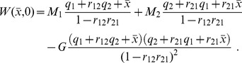
Considering relations (15) and (16) between efforts and probabilities, we obtain:

Two questions arise. Can we compare the true solution and the approximate solution? And can we estimate the error due to the approximation of the optimal solution? From Theorem 2, the upper bound on the error due to the approximation can be computed from the Hessian . In this two-species example, it is easy to derive the following formulae:

So the upper bound on the approximation error, indicated in Theorem 2, is:

(18)

a value which depends only on the number of genes owned jointly by the two species, , and on the ecological interaction terms,

Of course, this is only an upper bound. In some cases, the approximation could also give the exact solution. To illustrate this, assume as before that , that utilities are identical, and the upper bounds on efforts are the same for the two species, Assume also that the total budget can cover the protection cost of only one species, . Noah then has to choose among two extreme policies, the first one 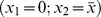that provides the following expected diversity:

and the second one with expected diversity:

It is optimal to protect species 2 if:

In the particular case where , then , and the above condition boils down to a very simple expression:

a condition which is also necessary for the approximated solution to select species 2 (remember condition (17)). It comes as no surprise that the optimal solution and its approximation concide, since when the upper bound on the approximation error is zero, as can be seen from expression (18).

Data Availability

The authors confirm that all data underlying the findings are fully available without restriction. All relevant data are within the paper and its Supporting Information files.

Funding Statement

This study was supported by the ONEMA program 2013-2015. The funders had no role in study design, data collection and analysis, decision to publish, or preparation of the manuscript.

References

- 1. Baumgärtner S (2004) Optimal investment in multi-species protection: interacting species and ecosystem health. EcoHealth 1: 101–110. [Google Scholar]
- 2. Baumol WJ, Bushnell RC (1967) Error Produced by Linearization in Mathematical Programming. Econometrica 35(3/4): 447–471. [Google Scholar]
- 3. Burgman MA, Ferson S, Akcakaya HR (1993) Risk Assessment in Conservation Biology. London: Chapman and Hall. pp 44–83. [Google Scholar]
- 4. Elith J, Leathwick JR (2009) Species distribution models: ecological explanation and prediction across space and time. Annual Review of Ecology, Evolution, and Systematics 40: 677–697. [Google Scholar]
- 5. Eppink FV, van den Bergh JCJM (2007) Ecological theories and indicators in economic models of biodiversity loss and conservation: A critical review. Ecological Economics 61(2–3): 284–293. [Google Scholar]
- 6.Garnett ST, Crowley GM (2000) The Action Plan for Australian Birds 2000. Environment Australia, Canberra, Australia.
- 7. Guisan A, Thuiller W (2005) Predicting species distribution: offering more than simple habitat models. Ecology Letters 8: 993–1009. [DOI] [PubMed] [Google Scholar]
- 8. Hauser CE, McCarthy MA (2009) Streamlining ‘search and destroy’: cost-effective surveillance for invasives species management. Ecology Letters 12: 638–692. [DOI] [PubMed] [Google Scholar]
- 9. Joseph L N, Maloney RF, Possingham HP (2008) Optimal allocation of resources among threatened species: a project prioritization protocol. Conservation Biology 23(2): 328–338. [DOI] [PubMed] [Google Scholar]
- 10. McCarthy MA, Thompson CJ, Garnett T (2008) Optimal investment in conservation of species. Journal of Applied Ecology 45: 1428–1435. [Google Scholar]
- 11. Simianer H (2008) Accounting for non-independence of extinction probabilities in the derivation of conservation priorities based on Weitzman's diversity concept. Conservation Genetics 9(1): 171–179. [Google Scholar]
- 12. Van der Heide MC, van den Bergh JCJM, van Ierland EC (2005) Extending Weitzman's economic ranking of biodiversity protection: combining ecological and genetic considerations. Ecological Economics 55: 218–223. [Google Scholar]
- 13. Weitzman ML (1998) The Noah's Ark Problem. Econometrica 66(6): 1279–1298. [Google Scholar]
- 14. Witting L, Tomiuk J, Loeschcke V (2000) Modelling the optimal conservation of interacting species. Ecological Modelling 125: 123–143. [Google Scholar]
Associated Data
This section collects any data citations, data availability statements, or supplementary materials included in this article.
Data Availability Statement