

Abstract
The thalamus relays sensori-motor information to the cortex and is an integral part of cortical executive functions. The precise distribution of thalamic projections to the cortex is poorly characterized, particularly in mouse. We employed a systematic, high-throughput viral approach to visualize thalamocortical axons with high sensitivity. We then developed algorithms to directly compare injection and projection information across animals. By tiling the mouse thalamus with 254 overlapping injections, we constructed a comprehensive map of thalamocortical projections. We determined the projection origins of specific cortical subregions, and verified that the characterized projections formed functional synapses using optogenetic approaches. As an important application, we determined the optimal stereotaxic coordinates for targeting specific cortical sub-regions and expanded these analyses to localize layer-preferential projections. This dataset will serve as a foundation for functional investigations of thalamocortical circuits. Our approach and algorithms also provide an example for analyzing the projection patterns of other brain regions.
INTRODUCTION
Anatomical connections provide structural substrates for information processing in the brain, yet neuroanatomical maps in most model organisms are incomplete1. This is especially true in mouse, where there are few comprehensive characterizations of anatomical connectivity despite being a primary model for studying neural function1. Anatomical connectivity at the mesoscopic level is critical for understanding of how circuits subserve behaviors and is necessary for investigation of circuit function using genetic manipulation1–3.
The thalamus is integral to the flow of information into and within the brain via its extensive interconnection with the peripheral and central nervous systems4–9. Thalamocortical projections are the primary drivers of cortical activity in sensory areas5 and associative brain regions, such as the frontal cortex10–12. The thalamus contains ca. 40 nuclei4,13,14, each innervating a different combination of cortical areas. Thalamic inputs to the frontal cortex are poorly characterized compared to thalamic inputs to primary sensory cortices, and our knowledge of the thalamo-frontal pathway is based on an amalgam of tracing studies from primates, cats, and rats spanning several decades4. Gaining a complete representation of each thalamo-frontal projection pathway from these studies has been difficult, due to variability between techniques and inconsistencies in anatomical boundary definitions4. A systematic characterization of thalamo-frontal pathways is necessary for investigating the function of frontal sub-regions.
It remains challenging to create a comprehensive thalamocortical projection map from individual thalamic subdivisions in mouse. First, the potential target area spans the entire cortex, necessitating a high-throughput microscopic method that can image the projections throughout the cortex at sufficiently high resolution and sensitivity1. Next, demarcating the cytoarchitectural boundaries for mouse thalamic nuclei is difficult because they are less distinct than the boundaries in other mammalian brains4. Furthermore, a comprehensive neuroanatomical dataset requires robust analysis methods to combine anatomical data across experimental animals15. Finally, it remains a major challenge to process, analyze, summarize, and present large anatomical datasets.
To overcome these challenges, we have developed a high-throughput approach using bilateral, two-color, anterograde, focal viral injections into mouse thalami. We then imaged injected brains at sub-micrometer resolution, providing single axon sensitivity. We developed algorithms to localize injections within a model thalamus, allowing us to compare injection and projection information across animals. We identified the origins of thalamic inputs to 19 cortical sub-regions in mouse, focusing on poorly understood thalamo-frontal pathways. We further localized the origins of layer-specific cortical projections to vibrissal motor cortex (vM1). Based on coordinates extracted from our analyses, we performed viral injections encoding channelrhodopsin, and optogenetically confirmed that the anatomically characterized projections form functional synapses. Our data provide a practical guide for viral injection, imaging, and manipulation of thalamocortical circuits in mice. This method and associated analyses can be adapted to develop comprehensive neuroanatomical connectivity maps in other brain regions.
RESULTS
Labeling and imaging thalamocortical projections
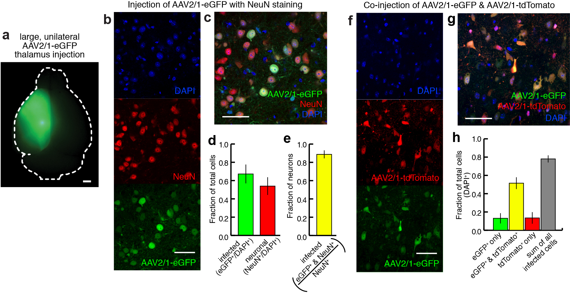
To visualize thalamic projections, we stereotaxically injected two recombinant adeno-associated viruses (serotype 2/1; AAV2/1)16–19 encoding eGFP and tdTomato respectively, bilaterally into the mouse thalamus (Fig. 1a–c and Supplementary Fig. 1) Thalamic projections do not cross the midline in mouse20 (Supplementary Fig. 1a), which allowed us to inject, image and analyze each hemisphere independently. Bilateral, two-color viral injections quadrupled the throughput of subsequent data collection, consolidated the total amount of data (~0.5 TB/animal), and eased computational demands for data processing. In addition, two-color labeling highlights topographic projection patterns from adjacent thalamic volumes21,22 (Supplementary Fig. 2). By using a hydraulic apparatus to deliver ~10 nL of AAV, a consistently small infection volume was achieved; measuring 0.30 ± 0.23 mm3, corresponding to ~1.6% of the total thalamic volume, and of 630 ± 160 μm (n = 188 injections) wide in the medial-lateral axis (Fig. 1c). 67.4 ± 10.3% of cells expressed detectable levels of fluorescent protein at the injection center, with an 88.8 ± 4.4% infection rate for neurons (Supplementary Fig. 1b–e).
Figure 1.

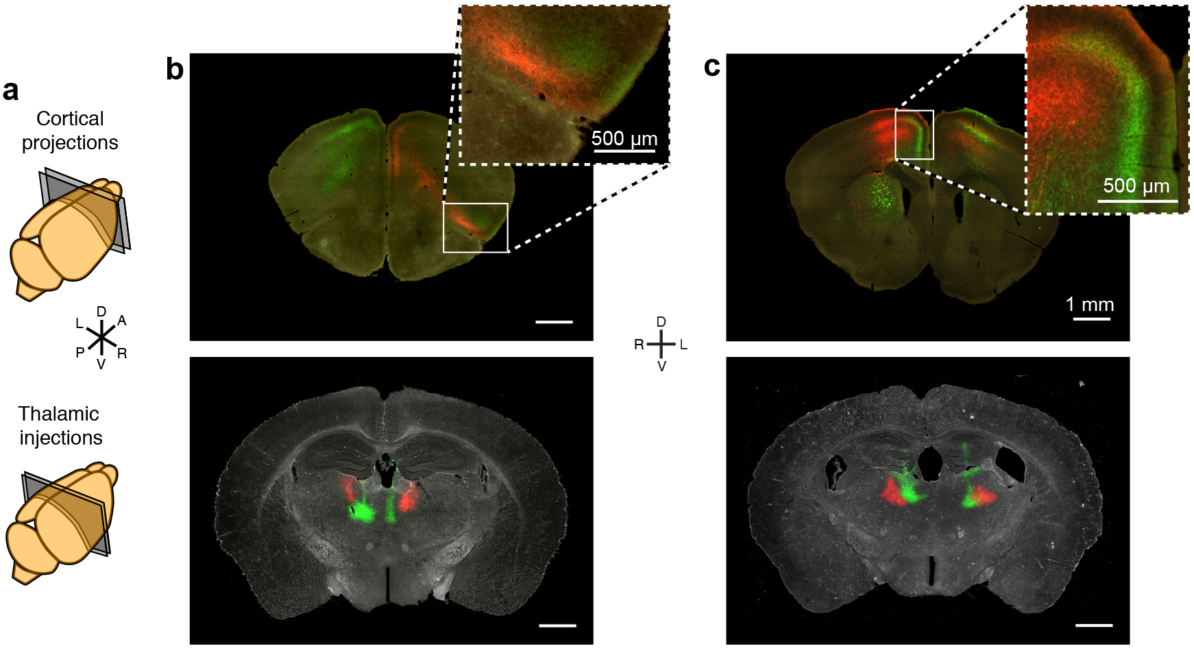
Systematic mapping of fluorescently labeled thalamocortical projections using high-throughput, high-resolution imaging. (a) Illustration showing bilateral viral injections driving the expression of tdTomato (red) and eGFP (green) in the mouse thalamus (left), followed by sectioning (50 μm/section, right) and high resolution imaging under identical conditions (right). (b) Representative coronal section showing thalamocortical projections to specific frontal subregions, with a zoomed-in image showing that full-resolution images allow the identification of single axons (inset). (c) Example fluorescent image showing viral injection sites on the dark-field image of the brain section (left). Solid white line: the thalamus mask. Zoom-in of the injection sites (right) shows the injection site masks created by intensity thresholding (solid line), as well as the injection site “cores” created by eroding the injection by 100 μm (dashed line) (see Methods). (d) The outline of the thalamus is manually traced in each coronal section and combined with the injection site masks created in panel c. These masks are then stacked to create a 3D representation of each thalamus. All scale bars are 1 mm, unless otherwise indicated. A (anterior), P (posterior), L (left), R (right), D (dorsal), V (ventral) throughout all figures.
Brains were paraformaldehyde fixed and cryostat sectioned coronally at 50 μm (Fig. 1a–c). All sections of each brain, from the start of the frontal cortex through the end of the thalamus, were fluorescently imaged in their entirety under identical conditions using a Hamamatsu Nanozoomer imaging system (0.5 μm/pixel) providing sufficient resolution to detect single axons (Fig. 1b). The thalami were re-imaged to avoid saturation of the injection sites (Fig. 1c). We successfully imaged 75 mouse brains containing a total of 254 injections, resulting in ~40 TB of imaging data.
An overview of data analysis
To analyze and compare thalamic injections across animals, we developed a suite of custom algorithms using MATLAB (MathWorks). The goal of these algorithms is to align individual injection sites onto a model thalamus (Fig. 1d), such that injection and projection information can be compared across brains. Supplementary Figure 3 schematically illustrates our approach. We manually traced each thalamus from the section images to generate a binary thalamus mask. Injection sites were masked by applying an intensity threshold to the images using a threshold determined by the Otsu’s method23 (Fig. 1c and Supplementary Fig. 3b). We then aligned and stacked each brain’s thalamus mask sections to create a 3D volume mask (Fig. 1d, Supplementary Fig. 4, and see Methods). We normalized the 3D masks and their corresponding injection site masks, corrected them for variability in cutting angle, and aligned them using anatomical landmarks (Supplementary Fig. 4, Supplementary Fig. 5, and see Methods). The aligned 3D thalamus masks were then averaged to produce a model thalamus (Supplementary Fig. 3c and Supplementary Fig. 6a), and each injection site was mapped onto the model (Fig. 1d).
We then determined the cortical projection targets for each injection, and combined the injection and target information for all 254 injections to localize the precise thalamic origin of the cortical projections (Supplementary Fig. 3d). We aligned two widely used atlases to the model for nucleus-specific analysis (Supplementary Fig. 3e). Notably, we also used our comprehensive dataset to create a nucleus-independent assessment of subdivisions within the thalamus (Supplementary Fig. 3e).
Assessment of thalamus alignment and injection coverage
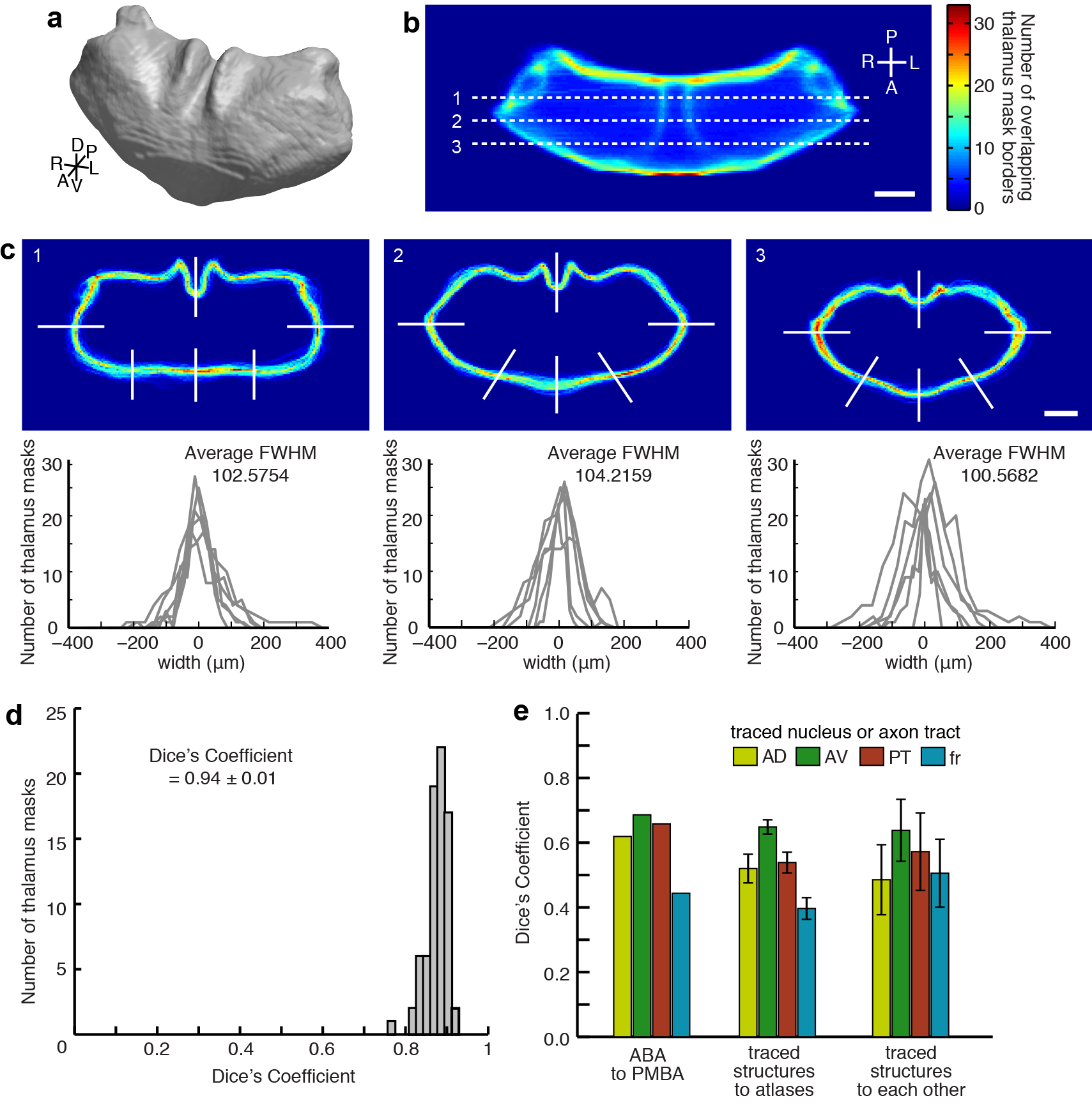
After normalization and alignment (see above and Methods), individual thalami were highly similar to each other, with only 3.7% variability in the thalamic volume (percent standard deviation), and 102 ± 51 μm (mean ± s.d.) variability in the thalamic border location (Fig 2a and Supplementary Fig. 6b–c). This variability is nearly identical to that measured with alternative data collection methods such as serial block-face imaging (102.5 μm ± 45 μm)24. The high degree of similarity between the individual masks and the model thalamus, was confirmed using Dice’s coefficient (D = 0.94 ± 0.01; Supplementary Fig. 6d). To facilitate subsequent data analysis, thalamus masks were down-sampled to a voxel size of 36.4 × 36.4 × 50 μm (x, y, and z, respectively), which is more than 2 fold smaller than the variability across individual thalami.
Figure 2.

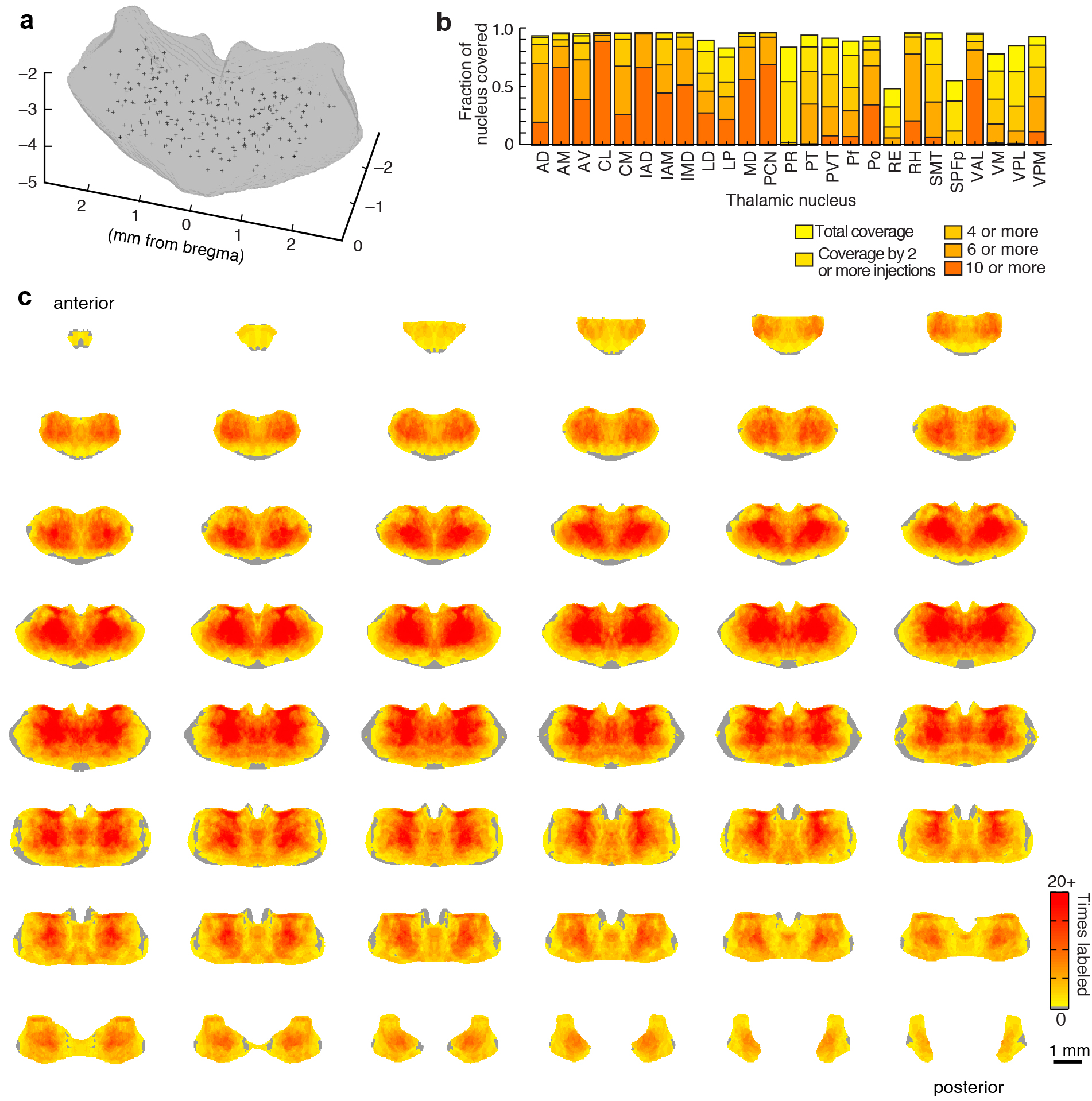
Assessment of variability across brains, atlas alignment, and injection coverage of the thalamus. (a) Top: aligned coronal thalamus sections from 75 brains (gray outlines). Black lines indicate 6 of 18 line profiles used to calculate thalamus edge variability. Bottom: thalamus edge variability after normalization at 18 locations (gray traces) and their average (black trace, full-width half-maximum = 102 ± 51 μm, arrowheads). (b) Two representative coronal sections through the averaged model thalamus (gray), overlaid with three thalamic nuclei (AD, yellow; AV, green; PT, red) and one axon tract (fr, blue) traced from 5 experimental brains. These atlas structures are also shown for the Paxinos Mouse Brain Atlas (PMBA, black) and the Allen Brain Atlas (ABA, white). (c) Dice’s similarity coefficient across the traced nuclei and axon bundle in 5 experimental animals, the ABA, and the PMBA, showing that each traced structure is well aligned to that same structure in other experimental brains and in each atlas. Data are symmetric across the diagonal. (d) The model thalamus (left) with coronal sections through the model thalamus showing injection coverage within the thalamus (i.e. how many times a voxel is hit by independent viral injections). See Supplementary Fig. 7 for full coverage maps. (e) The fraction of the thalamic volume covered by a given number of injections, with 93.4% of the thalamus covered by at least 1 injection (arrow). (f) The fraction of each thalamic nucleus covered by at least one and at least two injections. All scale bars are 1 mm.
We then aligned our model thalamus to two atlases: the Allen Brain Atlas (ABA, http://mouse.brain-map.org) and the Paxinos Mouse Brain Atlas (PMBA)25 (Supplementary Fig. 3e, Fig. 2b, and refer to Table 1 for all anatomical structure abbreviations). To verify this alignment, four cytoarchitecturally identifiable structures (AD, AV, PT and fr: all abbreviations are available in Table 1) were traced from 5 randomly selected experimental brains and compared to their corresponding atlas structures (Fig. 2b–c). The overall shape, orientation, and location of the thalamic structures were highly similar among the brains and atlases as quantified using Dice’s coefficient (Fig. 2c and Supplementary Fig. 6e). While variability across brains remained, the structures from experimental brains were as similar to the atlases (D = 0.53 ± 0.10) as the atlases were to one another (D = 0.60 ± 0.11; p = 0.35, t-test). We concluded that the alignment of individual nuclei to our model was accurate.
Table 1.
| Abbreviation | Paxinos location | |
|---|---|---|
| Thalamic nuclei | ||
| AD | anterodorsal nucleus | AD |
| AM | anteromedial nucleus | AM + AMV |
| AV | anteroventral nucleus | AV + AVDM + AVVL |
| CL | central lateral nucleus | CL |
| CM | central medial nucleus | CM |
| IAD | interanterodorsal nucleus | IAD |
| IAM | interanteromedial nucleus | IAM |
| IMD | intermediodorsal nucleus | IMD |
| LD | laterodorsal nucleus | LD + LDVL + LDDM |
| LG | lateral geniculate nucleus | VLG + DLG + VLG + IGL |
| LP | lateral posterior nucleus | LP + LPLR + LPMP + LPMC |
| MD | mediodorsal nucleus | MDC + MDL + MDM |
| MG | medial geniculate nucleus | MGD + MGV + MGM |
| PCN | paracentral nucleus | PC + OPC |
| Pf | parafascicular nucleus | Pf |
| Po | posterior nucleus | Po |
| PR | perireuniens nucleus | vRe |
| PT | parataenial nucleus | PT |
| PVT | paraventricular nucleus | PVA + PV |
| Re | reuniens nucleus | Re |
| Rh | rhomboid nucleus | Rh |
| SGN | supragenicualte nucleus | SG |
| SMT | submedius nucleus | Sub |
| SPFp | subprafascicular nucleus | SPFpc |
| VAL | ventral anterior-lateral complex | VA + VL |
| VM | ventromedial nucleus | VM |
| VPL | ventral posterolateral nucleus | VPL + VPLpc |
| VPM | ventral posteromedial nucleus | VPM + VPMpc |
| Cortical subdivisions | ||
| AI | anterior insular cortex | pregenual (AI + AID + AIV + DI + GI) |
| Aud | auditory cortex | Au1 + AuD + AuV |
| dACC | dorsal anterior cingulate cortex | Cg1 |
| FrA | frontal association area | FrA |
| IL | infralimbic cortex | IL |
| Ins | insular cortex | postgenual (AID + AIV + AIP + DI + GI) |
| LO | lateral orbital cortex | LO + DLO |
| M1 | primary motor area | M1 |
| M2 | secondary motor area | M2 |
| MO | medial orbital cortex | MO |
| Piri | piriform cortex | Pir |
| PrL | prelimbic cortex | PrL |
| Pt | parietal association cortex | MPtA + LPtA + PtPR + PtPD |
| Rhi | rhinal cortex | Ect + PRh + Lent |
| RS | retrosplenial cortex | RSA + RSG |
| S1/2 | sensory cortex | S1 (all sub-regions) + S2 |
| Tem | temporal association cortex | TeA |
| vACC | ventral anterior cingulate cortex | Cg2 |
| Vis | visual cortex | V1 (all sub-regions) + V2 (all subregions) |
| vM1 | vibrissal motor cortex | M2 |
| VO | ventral orbital cortex | VO |
We distributed the injections throughout the thalamus (Supplementary Fig. 7a) such that 93.4% of the thalamus was covered by at least 1 injection, and 85.3% was covered by at least 2 injections (Fig. 2d–f and Supplementary Fig. 7c). The majority of thalamic nuclei are fully covered (Fig. 2f and Supplementary Fig. 7b); however, we excluded the geniculate nuclei from the dataset. The center of the thalamus was more highly sampled because injections that extended beyond the lateral or ventral borders of the thalamus were excluded (Fig. 2d, and Supplementary Fig. 7a, c).
Mapping the thalamic origins to cortical targets
Using this dataset, we sought to identify the thalamic sources of projections to each of 19 cortical sub-regions of interest (ROI’s), which were defined by their boundaries in the PMBA (Fig. 3a). We noted the strength and specificity of projections from each of our injections to all cortical areas using a manual scoring system, as detailed in Supplementary Figure 8. Independently, three experts blindly performed this analysis.
Figure 3.

Localization of the thalamic origins of cortical projections. (a) Illustration showing the 19 cortical areas examined (modified from PMBA25 and reference 47): whole brain views (lower) and coronal sections (upper). (b) Simplified schematic of thalamic localization method: 1. The volume of each injection is eroded to generate an injection core (Fig. 1 and Methods); 2. Injections that send projections to a region of interest (ROI) (positive injections) are summed, and those that do not (negative injections) are subtracted; 3. Resulting in the precise thalamic volume projecting to each ROI, which is separated into eight confidence levels (Supplementary Fig. 8). (c) Example thalamus section illustrating the injection grouping method summarized in panel b. Sections 1 and 2: injections that do project and do not project to a target, respectively. Section 3: the refined thalamic volume projecting to that target (i.e. the confidence map). (d) Diagram of the thalamus sections shown in e. Coronal section −1.16 mm posterior to bregma (top), horizontal section −3.52 mm ventral to bregma (bottom). (e) Confidence maps (gray scale) show the thalamic origin of projections to nine frontal brain areas. See Supplementary Figure 9 for full confidence maps to all cortical areas. (f) Localization of exclusive and shared thalamocortical projections to PrL (green) and IL (magenta) through direct comparison of their confidence maps (right). Nuclear boundaries shown on left half of each thalamus section (PMBA). Coronal section −0.61 mm posterior to bregma (top), horizontal section −4.06 mm ventral to bregma (bottom). All scale bars are 1 mm.
We then used the projection scores for each injection to perform a simple injection site grouping method, which allowed us to localize the thalamic sub-volumes projecting to each cortical ROI. First, to account for the alignment variability between thalami (102 ± 51 μm), we eroded each aligned injection site by 100 μm to produce the injection “core” (Fig. 1c, and Fig. 3b). The core, as compared to the periphery, represents the volume of an injection that we are more confident is accurately localized within the model thalamus.
Next, we combined the volumes of all injections that projected to a given ROI (“positive” injections), and then the volumes of the injections that did not project to that region (“negative” injections) were subtracted from the combined total. This process resulted in a better localization of the thalamic volume projecting to each ROI than if the summed positive injection volume was used alone (Fig. 3b–c and Supplementary Fig. 8e–g). By employing this method, we localized volumes at a finer resolution than at the size of a single injection. The grouping method described above was expanded to assign higher confidence to injection site cores, as well as account for different projection properties, such and strength and specificity (see Supplementary Fig. 8 and Methods for detailed grouping). This analysis resulted in confidence maps in which the value of each thalamic voxel, volumetric pixel, indicates our certainty that the thalamic voxel projects to a particular ROI (Fig. 3d–e and Supplementary Fig. 8d–g), where a confidence value of 8 is highest, and a confidence value of 0 means that no projections originated from that voxel. We have provided confidence map summaries for the nine sub-regions of the frontal cortex: FrA, dACC, vACC, PrL, IL, MO, VO, LO, AI (Fig. 3d–e, Supplementary Movies 1–9, and Supplementary Fig. 9 for full confidence maps to all sub-regions). Each confidence map contains a continuous positive volume, which is unique for each target region. To validate the projection sources predicted by our confidence maps, we performed injections of fluorescent retrograde beads in a subset of our characterized areas (Supplementary Fig. 10). We observed all retrogradely transported beads were localized within the predicted confidence map.
One advantage of having confidence maps across many cortical sub-regions is that we could directly compare the thalamic origins of functionally related cortical sub-regions. For example, PrL and IL are both crucial in fear learning, but PrL is associated with the ‘high fear’ behavior state, and IL is associated with the ‘low fear’ state26. By comparing the confidence maps for PrL and IL, we localized the shared and unique thalamic origins to PrL and IL (Fig. 3f), suggesting that differential thalamic inputs may contribute to their functional differences. Such comparisons allow for the selective targeting of thalamic projections to PrL and IL for future functional studies.
Defining thalamic subdivisions based on cortical targets
The thalamus is commonly subdivided into anatomically and functionally similar nuclear groups4. While useful, these divisions ignore ambiguity in nuclear borders, differences in projection patterns within a single nucleus, and the possibility that cytoarchitecturally defined nuclei may not always be the relevant functional unit within the thalamus5. Since our confidence maps provide distinct topographic information (Fig. 4a), we determined whether the thalamus could be instead sub-divided based on cortical projection patterns alone.
Figure 4.

Localizing thalamic subdivisions based on cortical projection patterns. (a) Summary of confidence maps to all cortical sub-regions, clustered based on confidence map similarity (determined in panel c). See Supplementary Fig. 9 for large confidence maps. (b) The thalamus is down-sampled into 150 × 150 × 150 μm voxels (left) and the average confidence level within each voxel is determined for each cortical projection (example, right). (c) All thalamic voxels (rows) are hierarchically clustered based on their cortical projection patterns, and cortical subregions (columns) are clustered based on which thalamic voxels innervate them. The average confidence level is indicated in gray scale, as in a. A threshold (gray dashed line, left) was applied to identify 11 distinct clusters. (d) Coronal thalamus sections showing the spatial location of clusters from c (left), with the corresponding atlas sections (PMBA, left half & ABA, right half) showing thalamic nuclear groups for comparison (right). (e) Schematic showing the convergence and divergence of projections for several clusters. (f) Overlap between voxel clusters (rows) and atlas-defined nuclear groups (columns). Colored boxes highlight the clusters that are dominant in (compose >10% of) the anterior and medial thalamic groups. Some nuclear groups are covered by relatively few clusters that have closely related projection patterns (e.g., the anterior group mainly contains clusters 1 and 2), while other groups contain clusters with disparate projection patterns (e.g., the medial group contains clusters 2 & 5–10). (g) Coverage of the anterior and medial nuclear groups by each voxel cluster.
The thalamus was divided into 150 × 150 × 150 μm voxels (Fig. 4b), which were then clustered (agglomerative hierarchical clustering, MATLAB) based on their confidence values for all 19 cortical sub-regions (Fig. 4b–c). We then applied a threshold to identify the 11 largest thalamic voxel clusters (Fig. 4c–e). Notably, the thalamic voxels comprising each cluster were spatially grouped and largely continuous, and similar to the thalamic nuclear groups (Fig. 4d). However, the voxel clusters and nuclear groups were not identical. While several nuclear groups were comprised of one or two closely related clusters (Fig. 4f–g, anterior and intralaminar nuclear groups), other nuclear groups contained several largely divergent clusters (e.g. the medial and ventral groups, Fig. 4f–g), suggesting functional homogeneity in some nuclear groups, but significant heterogeneity in others.
Optimal injection sites and functional confirmation
Stereotaxic viral delivery of optogenetic and pharmacogenetic reagents to manipulate neuronal activities has become an important method to dissect functional circuitry. Currently, studies involving the mouse thalamus that employ these methods primarily rely on the empirical determination of the injection coordinates based on a small number of trials. Using the confidence maps developed here, we have simulated injections throughout our model thalamus and determined the optimal injection coordinates for targeting projections to a specific ROI (Fig. 5a and Supplementary Fig. 11 for all optimal injection coordinates).
Figure 5.

Targeting anatomically defined thalamocortical projections to verify that they form functional synapses. (a) Optimal injection coordinates for dACC, i.e. the most probable location to inject in order to target thalamic projections to dACC, determined from the confidence maps in Fig. 3. Anterior (left), dorsal (middle), and lateral (right) views of the target thalamic volume. (See Supplementary Fig. 11 for details). Shown in millimeters relative to bregma. (b–c) Optimal injection coordinates were used to target thalamic projections to dACC. (b) Image of thalamic axons expressing fluorescently-tagged channelrhodopsin 2 (ChR2) in dACC. Orange circles indicate the location of two neurons recorded sequentially in layers 1 and 2/3 of dACC during optogenetic activation of the ChR2 expressing thalamic axons. White stars indicate the location of ChR2 stimulation by blue light (8 × 12 grid, 50 μm spacing). (c) Current recordings of the two neurons shown in panel b, showing synaptic currents elicited by light stimulation of thalamic axons. Each current trace corresponds to the white star grid in panel b rotated 30° counter-clockwise. The center of each circle indicates the location of the cell body. (d) The approximate locations of all neurons recorded (white circles) are shown, and crossed circles indicate no postsynaptic response. The approximate position shows the cortical layer (superficial: layer 1, middle: layers 2–4, and deep: layers 5–6), and the anterior-posterior extent of each area is collapsed into a single section (schematic modified from PMBA).
Since anatomical projections do not always guarantee functional connectivity16,27,28, we sought to verify that the observed anatomical axonal projections form functional connections at each target region, which also allowed us to verify the validity of the optimal injection coordinates. We injected AAV2/1 expressing channelrhodopsin2 (ChR2) using our optimal injection coordinates to target thalamic projections to eight frontal sub-regions. Whole cell recordings were made in each projection target area, shown here for dACC (Fig. 5b), and postsynaptic responses were observed upon activation of the ChR2+ thalamic axons with blue light stimulation (Fig. 5b–d and Methods). 48 out of 50 cells recorded showed excitatory responses; specifically, we recorded responses from 4/4 cells in AI, 13/13 in VO/LO, 4/4 in MO, 3/5 in IL, 5/5 in PrL, 19/19 in dACC/vACC (cells with responses/total cells recorded; Fig. 5d), indicating that the anatomically defined projections corresponded to functional thalamocortical synaptic connections.
Grouping thalamic nuclei based on cortical targets
As described earlier, nucleus locations from both the ABA and PMBA were aligned to our model thalamus (Fig. 2b–c), allowing us to localize the origins of cortical projections to individual nuclei (Fig. 6a–c). To compute the fraction of each nucleus that projects to a given ROI, the nuclear boundaries aligned from the atlases were overlaid onto the confidence maps (Fig. 6b), and the coverage of a given nucleus was averaged between the two atlases. The coverage distribution across nuclei is shown for projections to select frontal sub-regions (Fig. 6a, d and see Supplementary Fig. 12 for all areas). We performed a cluster analysis using the nuclear localization of the confidence data for all 19 cortical sub-regions to identify projection patterns across thalamic nuclei (Fig. 6e). Functionally related cortical sub-regions formed tight clusters when grouped according to the origin of their thalamic inputs, suggesting that our comprehensive anatomical dataset can be predictive of functional relationships, which validates our approach. It is important to note that there are limits to the resolution of this method: small (<300 μm wide) and intricately shaped nuclei will be difficult to separate from their neighbors.
Figure 6.

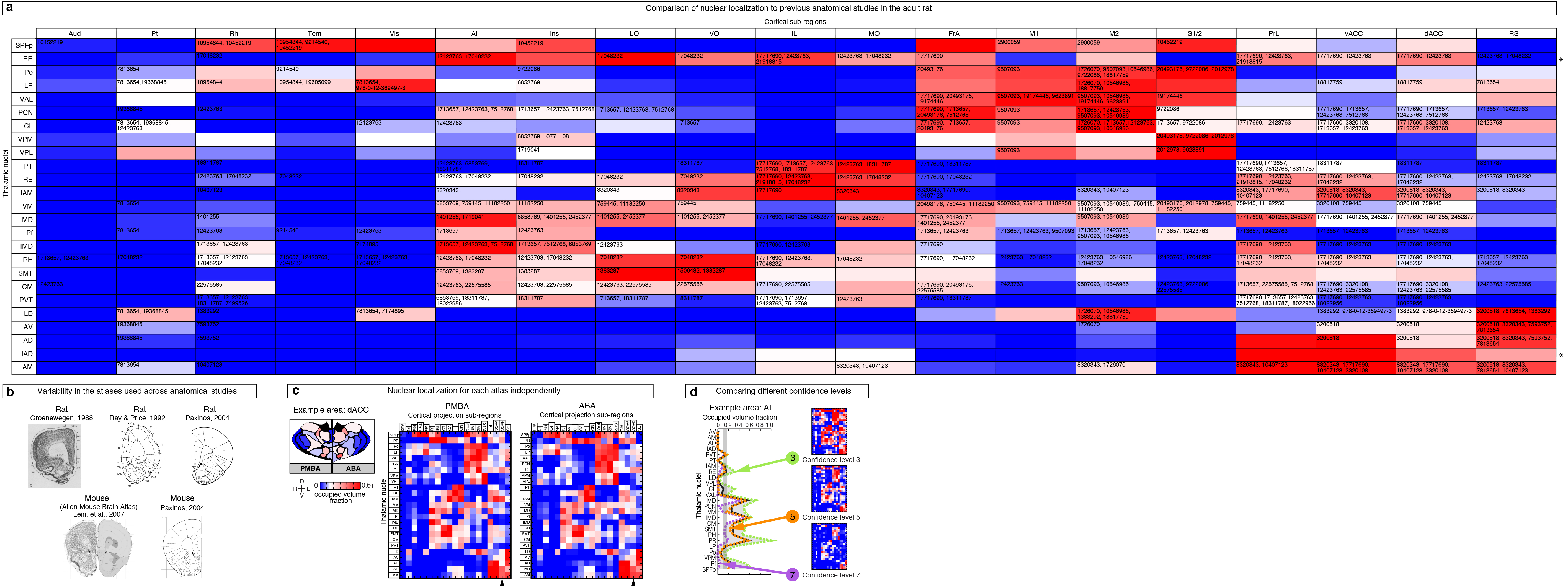
Nuclear localization of the thalamic origins of frontal projections. (a–c) Three representations of the nucleus origin data for LO (See Supplementary Fig. 12 for remaining cortical sub-regions). (a) The fractions of each thalamic nucleus projecting to LO are shown in three confidence levels (dashed lines) with their average (black line). Vertical gray line: the inflection point in the color scale used in panels b, c, and e. Asterisks indicate potential differences between localized thalamocortical projection origins and literature data in rat (see Supplementary Fig. 13a for details). (b) Single coronal section through the confidence map for LO (gray scale) overlaid with nuclear subdivisions from the ABA. The atlas is colored on the left to indicate the fraction of each nucleus covered by the average confidence trace (black line in panel a), with the inflection point (white) at 15%. (c) Spatial representation of all nuclei projecting to the LO. Circle diameters correspond to the relative size of each nucleus and their positions correspond to their relative center-of-mass location within the thalamus in the anterior-posterior and medial-lateral axes. Color scale is the same as in panel b. (d) The fractions of each thalamic nucleus projecting to AI, IL, and FrA, shown in three confidence levels (dashed lines) with their average (black line), as described in panel a. (e) Aggregate nucleus coverage map for all cortical areas. Nuclei (rows) and cortical sub-regions (columns) are hierarchically clustered based on output and input similarity, respectively. Color scale is the same as panel b.
We compared our nuclear localized thalamocortical projection data to literature data for rat (Fig. 6a, d, Supplementary Fig. 12 and Supplementary Fig. 13), because primary anatomical data for mouse is sparse4. Overall, our nucleus projection data are largely consistent with the cumulative rat anatomical data, but we have indicated discrepancies between our findings and the rat literature with asterisks (Fig. 6a, d and Supplementary Fig. 13a for full literature list). Several factors may contribute to these discrepancies. First, the boundary definitions between cortical sub-regions vary across atlases, so the atlas used in each study will impact their findings (Supplementary Fig. 13b)25,29–31, as exemplified by FrA25,31–33. Second, localization of projection origins within specific thalamic nuclei can vary both due to the atlas used and the ability to precisely target individual nuclei, as demonstrated by the discrepancies in projections from CM reported in the literature20,32,34–36 (Supplementary Fig. 13a). To avoid anatomical bias, we averaged nucleus localization data between two atlases (ABA and PMBA) (Supplementary Fig. 13c), and created our confidence maps independent of nuclear boundaries (Fig. 3e). In addition, most studies cannot identify the regions of the thalamus that do not project to a given ROI because they lack the comprehensive dataset necessary to do so. Using our approach, we are able to present this underreported feature of the thalamocortical connectome (Fig. 6 and Supplementary Fig. 12).
Thalamic origins of layer-preferential projections in vM1
Different layers of the same cortical area play distinct roles in information integration. We analyzed the primary vibrissal motor cortex (vM1) to test whether our dataset could be used to identify thalamic volumes preferentially innervating specific cortical layers. We previously showed that the posterior “sensory” thalamus is more likely to project to layers 2/3 and 5a (L2/3–5a) in vM1, whereas the anterior “motor” thalamus projects to layer 5b (L5b) as well as L2/3–5a37. However, we had to estimate the thalamic volumes responsible for these projections based on subjective assessments of a small number of injections.
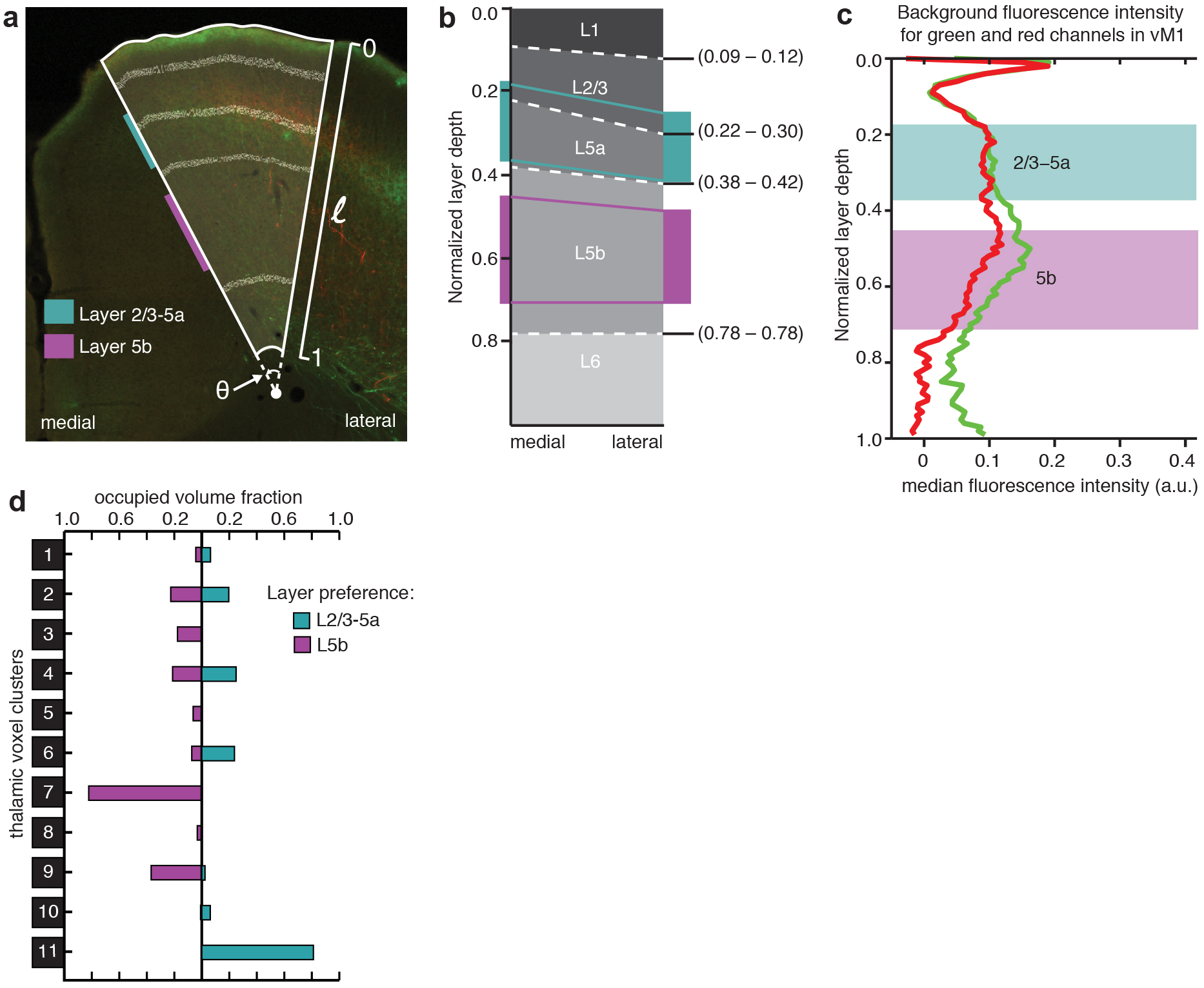
To accurately localize the thalamic origin of layer-specific projections to vM1, we quantified the fluorescence intensity of thalamic projections to L2/3–5a and L5b for each injection (Fig. 7a–c and Supplementary Fig. 14), and created modified confidence maps to characterize the thalamic volumes associated with layer preferential projections (Fig. 7d–e and Methods). Several nuclei, including PCN, AM, LD, and VAL, contained volumes preferentially innervating L5b (Fig. 7d–g). While previous research shows that these nuclei send vM1 projections broadly to both L5b and L2/3–5a37, we found the first evidence of preferential projections to L5b in vM1. Since L5b neurons provide the only direct motor output from vM1, these projections may play a direct role in motor control. The thalamic projections that preferentially target L2/3–5a arose from a more posterior-central thalamic volume, identified here as Po, LP, Pf and SPFp (Fig. 7d–g). This confirmed previous results, which suggest preferential projections from a region containing Po to L2/3–5a in vM137. Furthermore, when we compared each layer-preferential thalamic volume to the thalamic voxel clusters identified in Figure 4c, we found that several clusters displayed strong preference to specific vM1 layers. For example, 81% of cluster 11 preferentially projected to L2/3–5a of vM1, while only 0.3% projected preferentially to L5b (Supplementary Fig. 14d). We concluded that future studies can use our method to identify thalamic volumes targeting detailed anatomical features.
Figure 7.

Cortical layer preferences of thalamic projections to primary vibrissal motor cortex (vM1). (a) Coronal brain section showing layers 2/3 and 5a (L2/3–5a, cyan) and layer 5b (L5b, magenta) in vM1 (white dashed outline). (b) Example coronal sections of vM1 (left image magnified from panel a), showing thalamocortical projections with preference to L5b (red projections, left), and L2/3–5a (red and green projections, right). (c) Normalized fluorescence intensity plots for red and green projections in panel b (left image: dashed lines, right image: solid lines). Fluorescence is averaged radially across vM1 to determine layer preference (see Methods and Supplementary Fig. 14). Background fluorescence is calculated from brains without vM1 projections (gray line). (d) Dorsal (left) and oblique (right) views of a 3D thalamus rendering, showing the volumes that are associated with preferential axonal projections to L2/3–5a (cyan) and L5b (magenta). The total volume projecting to all layers of vM1 is shown (gold dashed line). (e) Representative coronal (left) and horizontal (right) sections of modified confidence maps for L2/3–5a (cyan) and L5b (magenta) preferential vM1 projections. Outlines of thalamic nuclei are overlaid on each section image. (f) The occupied fraction of each thalamic nucleus containing layer-preferential projections to L2/3–5a and 5b of vM1. An arbitrary 10% threshold is indicated (gray line). (g) Schematic showing layer preferential input from thalamus to vM1 in the context of a motor-sensory circuit diagram. All scale bars are 1 mm.
DISCUSSION
Mesoscopic connectivity maps are crucial for studying interactions among multiple brain regions and for linking cellular circuit mechanisms to behaviors. In this study, by using anterograde viral tracing, high-throughput whole brain imaging, and custom development of alignment and analysis software, we established a mesoscopic thalamo-centric projection map to the cortex in mouse, identified unique thalamic sub-volumes projecting to each cortical subregion, and determined the optimal injection coordinates for optogenetically or anatomically targeting specific cortical regions. Our maps also permitted the identification of shared and unique thalamic sources to different cortical regions, such as PrL and IL (Fig. 3f), providing an entry point for teasing out their common and distinct functions. Additionally, our systematic approach allowed us to functionally subdivide the thalamus based solely on cortical projection patterns (Fig. 4). We further identified the thalamic volumes that give rise to layer-preferential projections to vM1 (Fig. 7). Our results provide a foundation for understanding the function of the thalamus and frontal cortex, as well as for investigating and manipulating the microcircuits within and between thalamic and cortical sub-regions.
Historically, the extensive time and labor required to image and map long-range projections limited the number of tracer injections used in anatomical studies, and necessitated the reliance on subjective assessments to compare across experiments. Recent advances in high-throughput fluorescent imaging facilitate the generation of large anatomical image datasets22,38–40, allowing researchers to access vast amounts of anatomical information. However, extracting relevant biological information from these data remains a major challenge for several reasons: variability across experiments, both due to intrinsic size differences and experimental manipulation, makes it difficult to compare across experiments directly; the resolution is limited to the size and shape of the tracer injection site; and the tools needed for data analysis have not kept up with technological advances in data collection, impeding efforts to turn images into knowledge.
We addressed variability issues by tightly controlling the animal age (P30 ± 2), computationally correcting for angled sectioning, and normalizing individual thalami to a standard volume. The variability among our thalamic mask boundaries is 102 ± 51 μm, comparable to that observed in the absence of mechanical sectioning24. By creating a comprehensive, age-matched thalamocortical projection map, we have provided a framework that others can build upon to understand differences across age groups, cell types, and species. These variances may explain some of the discrepancies seen across the 43 anatomical studies we evaluated in rat and our data in mouse (Supplementary Fig. 13).
Another major limitation of mesoscopic mapping is that the size of the tracer injection limits the resolution. To reliably identify the origin of the each mapped projection, tracer injections must target a single defined brain region. This is straightforward in cortical areas with large, superficial sub-regions 39,40; however, this task is difficult, if not impossible, in the thalamus due to the complex shape and small size of many thalamic nuclei. We overcame this limitation by analyzing the intersectional areas of overlapping injections (Fig. 3b–c), which allowed us to localize volumes smaller than a single injection. We could only have obtained our confidence maps and optimal injection coordinates by integrating information from a large number of highly overlapping injections. Furthermore, to maximize our resolution, we used the smallest replicable viral infection volume (~0.3 mm2, and laterally ~600 μm). We estimated our resolution to be larger than our variability (~100 μm) and smaller than our injection size (~600 μm), which is sufficient for most thalamic targeting, but small thalamic nuclei may require smaller injection volumes or more closely spaced injections to precisely discriminate their boundaries (e.g. Supplementary Fig. 10). Because of the heavy dependence on viral infection to deliver molecular reagents in systems neuroscience, our map, which is at the equivalent ‘operational scale’, can serve as a guide for targeting these tools.
By exploiting injections that both do and do not project to each cortical ROI, we were able to identify the entire thalamic volume that does not project to each cortical ROI. From an anatomical point of view, characterization of non-projecting regions is particularly important because it has been estimated that only ~10% of all possible connections within the rodent brain are fully characterized at the mesoscopic level, largely due to a lack of definitive information on non-existent projections1.
As stated by Sherman and Guillery, ‘The concept of the thalamic nucleus as a single structural, functional, and connectional entity has barely survived advancing techniques and new information. We stay with the thalamic nuclei as one of our prime analytical tools because, as yet, we have little to use in its place’. Here, our comprehensive projection map provided us with a unique opportunity to establish a nucleus-independent map of thalamic projections that transcends what we have learned from a nucleus-based framework (Fig. 3–5). Although we related our results to thalamic nuclei, we created our confidence maps independent of nuclear boundaries. This enabled us to unbiasedly identify the precise thalamic volumes responsible for projections to specific cortical sub-regions and cortical layers.
Our maps were obtained in adolescent mice, which is a dynamic period for prefrontal cortex (PFC) associated behaviors41–43. We found that thalamocortical projections from at least 25 nuclei have reached PFC and form functional synapses by P30 (Fig. 5 and 6). Since the frontal sub-regions innervated by each nucleus are comparable to those seen in the adult rat (Supplementary Fig. 13), our data suggest that thalamocortical projections to PFC have reached their final targets by P30 in mouse. We therefore propose that the behavioral changes that occur during adolescence are more likely due to local refinements and synaptic pruning than larger rearrangements in thalamocortical projection distributions to PFC sub-regions.
In light of novel tools for imaging, physiology, and cell-type specific manipulations in mouse2, the mesoscopic data provided here will serve as a critical reference for applying these tools to study circuit function. The results from over 43 disparate studies were necessary to summarize only a fraction of the thalamocortical projections in rat that are described here in mouse (Supplementary Fig. 13), which is a testament to the power of the high-throughput imaging and computational analyses used in this study. The ability to directly compare across animals and experiments is a crucial step for extracting useful biological information from large anatomical datasets. Our results present an example for large-scale data integration and analysis, and will inform future studies in systems neurobiology.
Online Methods
All animal experiments were conducted according to National Institutes of Health guidelines for animal research and were approved by the Institutional Animal Care and Use Committee. All measurements are listed as mean ± standard deviation, unless otherwise indicated. All calculations were performed in MATLAB (MathWorks). The raw data and the analyzed data are publicly available at http://digitalcollections.ohsu.edu/projectionmap. The original resolution images are available upon request as hard drive format.
Stereotaxic viral injections
Injections were performed as described16 with optimizations/modifications. Briefly, C57BL/6J male and female mice were anesthetized (1–2% isoflurane) at P14–18 and stabilized in a custom stereotaxic apparatus (modified from a David Kopf system). A dental drill (Henry-Schein) was used to drill holes through the skull. A pulled glass micropipette (Drummond; tip diameter: 10–15 μm), beveled sharp, was backfilled with AAV (serotype 2/1) that expresses either eGFP (Addgene 28014) or tdTomato (A gift from J. Magee). AAV2/1 is a hybrid serotype that has AAV2 inverted terminal repeats, AAV1 capsid proteins, and widespread neuronal tropism17. The transgenes were driven by CAG promoter and included a WPRE element to enhance the expression. The viruses were prepared by the University of Pennsylvania vector core and viral titers >5.0 × 10¹² GC/mL were used. Unless noted otherwise, a 10 nL volume of virus was dispensed at a speed of 5 nL/s using a hydraulic injector (Narishige), followed by a 5–10 minute waiting period. The pipette was retracted 0.3 mm at 0.008 mm/s, paused for 3 minutes, and then retracted at a rate of 0.008 mm/s. This process minimized the undesirable infection of cells along the injection path. Up to four injections were performed in each animal (two colors and two hemispheres). Coordinates for injections ranged from: 0.5 – –1.6 anterior to posterior, 0 – 1.6 lateral, and 2.8 – 4.2 deep from the pia (in mm from bregma). Although no statistical methods were used to pre-determine sample sizes, we sought to insure that the final coverage of all thalamic labeling was > 90%. We found that this could be achieved via 254 highly-overlapping injections across 75 animals.
Sectioning and imaging
14 days after viral infection, mice were perfused transcardially with 25 mL phosphate buffered saline (PBS) followed by 50 mL of 4% paraformaldehyde (PFA). The brain was post-fixed in 4% PFA at 4°C overnight and then placed in 30% sucrose in PBS at 4°C overnight. The brain was centered and aligned in a rectangular mold, embedded in Optimal Cutting Temperature medium (TISSUE-TEK), and sectioned coronally on a cryostat (Thermo Scientific) at 50 μm thickness. The sections from the most anterior section of the cortex to the most posterior section of the thalamus were floated in PBS and then collected onto Superfrost-Plus microscope slides (FisherBrand). Slides were mounted using Fluoromount (Sigma) and covered with number 1.5 cover glass (Gold Seal, Fisher).
All sections on the slides were imaged with a 20X objective (0.5 μm/pixel) on the Nanozoomer slide scanner (Hamamatsu), at a fixed exposure time. Because injection sites were often overexposed under these settings, they were re-imaged at a lower exposure with either a 5X objective on a Zeiss Axio Imager or using shorter exposure times on the Nanozoomer. Axio images were matched to their corresponding Nanozoomer section images through rigid translation and rotation using manually selected anatomical landmarks visible in both images. After imaging, injections that extended beyond the lateral or ventral borders of the thalamus were excluded. Each brain was processed and imaged equivalently and randomly without any knowledge of the injection locations.
Cell counting
Confocal images were collected (Zeiss, LSM780) for DAPI (Vector Labs) stained sections across the center of an AAV2/1-eGFP thalamic injection site from 17 mice. The fraction of cells found to be both DAPI- and eGFP-positive indicated the percentage of DAPI-positive cells infected (Supplementary Fig. 1d). To calculate the percentage of neurons infected, thalamus sections across the center of AAV2/1-eGFP injections from 5 mice were incubated with mouse anti-NeuN (Millipore), followed by Alexa-594 goat anti-mouse secondary antibody (Life Technologies) and DAPI. The fraction of DAPI-positive cells that were also NeuN- and eGFP-positive indicated the percentage of infected neurons at the injection site (Supplementary Fig. 1b–e). To confirm these results, the thalamus sections from 3 mice injected with eGFP-expressing AAV2/1 were stained with NeuroTrace (Life Technologies) and DAPI and were analyzed in the same fashion (data not shown). To evaluate the viral tropism, eGFP and tdTomato expressing AAV were mixed (1:1) and co-injected into the thalamus in 4 mice. The same imaging process was used as with single viral injections (Supplementary Fig. 1f–h).
Thalamus and injection site segmentation
Individual sections were isolated from the full slide images by determining an intensity threshold that would distinguish tissue from background pixels. The outline of the thalamus was manually traced to generate a thalamus mask (Fig. 1c). The front of the thalamus was defined as the first slice posterior to the anterior commissure (AC) crossing the midline, and the back of the thalamus was defined as one slice posterior to the end of the lateral geniculate nucleus (LGN) 25,31. In addition, the medial and lateral geniculate nuclei were not included due to their already well-characterized anatomy in the auditory and visual systems, respectively. Finally, the posterior portion of the reticular thalamic nucleus (RT), which does not produce cortical projections44 and the posterior portion of the ventral medial nucleus (VM) were excluded from the traced masks due to technical difficulties in visualizing their borders. We segmented each injection site into a binary mask by applying independent intensity thresholds in green and red channels, utilizing a supervised MATLAB routine based on Otsu’s method23. Traveling axon bundles that were above threshold in the thalamus were manually excluded from the associated injection site.
Thalamus registration and alignment
The model thalamus and registered injections were created as described in Supplemental Table 1. 1) Two manually selected midline points were used to rotate and align the thalamus masks. 2) To align the masks in the correct y position and to correct for the cutting angle tilt about the x-axis (i.e., rotation around the x-axis), we used anatomical landmarks to estimate the tilt angle (Supplementary Fig. 5). A separately traced ABA thalamus mask was rotated to the same tilt angle and the mask stack was resampled as 50 μm slices. 3) The centers of mass of these slices were used to direct the position of experimental thalamus masks in y. The center of mass is defined as the unique point where the weighted relative position of the distributed mass sums to zero and was calculated as the following:
where M is the sum of the masses of each point r in a volume V with constant density ρ(r).
The aligned thalamus masks were then rotated to a tilt angle of 0 degrees and re-sampled as 50 μm slices (Supplementary Fig. 5). The thalamus masks were down-sampled to a 36.4 × 36.4 × 50 μm voxel size. 4) To control for the cutting angle tilt about the y-axis, the aligned 3D mask was sheared to maximize left and right asymmetry. 5) The overall size of the thalamus was scaled: i) in z so that the midline distance from the beginning to end of the thalamus matched the ABA thalamus, ii) in x-y isotropically to match the total area of the central slices with that of the corresponding ABA thalamus, and iii) the 3D thalamus masks were scaled in x to match the average width of all thalamus masks. 6) The masks were visually inspected and 18/75 brains underwent minor scaling or position adjustments in the z dimension. All brains were further aligned with each other in y based on their center of mass. All experimental masks were summed and then segmented according to a threshold that retains the volume of averaged thalamus mask volumes, producing the model thalamus.
We used Dice’s coefficient to assess the similarity between two thalamic structures (Fig. 2c and Supplementary Fig. 6d). Dice’s coefficient is defined as
where A and B are two binary volumes, ‘&’ is the logical AND operator and ΣX indicates the sum of all elements in X45. To further quantify the variability of thalamus masks (Fig. 2a and Supplementary Fig. 6), we overlaid the borders of each thalamus mask and measured the distribution of boundary points at 18 locations (6 locations per slice for 3 z slices). Injection site masks were processed identically to their corresponding thalamus masks so that they are registered to the model thalamus. All injection site masks were summed to quantify the injection coverage at individual voxels (Fig. 2d–f). Data distribution was assumed to be normal but this was not formally tested.
Atlas Alignment
To register known thalamic nuclei within our model thalamus, we traced, scaled, and re-sampled 25 nuclei from both the ABA and PMBA as 3D volumes that are aligned with our model thalamus. Differences in animal age and tissue preservation techniques resulted in size and shape differences between the two atlases, so each atlas was scaled separately to best fit our model thalamus. The correspondence between the nuclei of individual experimental thalami and the atlas nuclei were assessed by manually tracing four cytoarchitecturally identifiable thalamic structures (nuclei AD, AV and PT and fiber tract fr) from five randomly selected brains (Fig. 2b). The similarity between the atlas and experimental nuclei was assessed using Dice’s coefficient (Fig. 2c and Supplementary Fig. 6e). Notably, the values of Dice’s coefficients for comparing nuclei in are lower than those for comparing the thalami of all brains (Supplementary Fig. 6d–e) because this coefficient is inversely dependent on volume. For example, the average volume of the traced nuclei is 0.24 mm3 (1.3% of the model thalamus volume), and our position variability (~100 μm) affects D for nuclei more than for the larger thalamus masks. The similarity matrix shows that (1) each traced nucleus is more similar to a corresponding nucleus in another brain or atlas, than to other nuclei, (average D = 0.53 for comparing the same nuclei and D = 0.02 for comparing different nuclei) and (2) similarities between traced nuclei and atlas nuclei (D = 0.53 ± 0.10) are comparable to that of the atlases to each other (D = 0.60 ± 0.11) (Fig. 2c and Supplementary Fig. 6e).
Confidence maps and thalamic origins of projections to the cortical sub-regions
For each thalamic injection, projection distributions were blindly scored by three independent experts. The presence/absence, strength (dense or sparse), coverage (full or partial ROI coverage), and specificity (whether the projection also goes to an adjacent ROI) were determined (Supplementary Fig. 8b). All final scoring decisions were reached by consensus. The cortical area boundaries were based on the PMBA. Injections are referred to as being “positive” or “negative” for a given cortical ROI, where “positive” indicates the presence of a projection and “negative” indicates the absence of a projection for this particular ROI. To control for our alignment variability (~100 μm) across thalamus masks (Fig. 2a and Fig. 3b), an injection core was produced by eroding each 3D injection mask by 100 μm.
A confidence map, which defines the thalamic origin of cortical projections, was created for each target projection region. As shown in Supplementary Figure 8, a confidence map was developed by grouping injections (Fig. 3b) that met each of eight independent criteria. Meeting each criterion would give a thalamic voxel a score of 1 and meeting all criteria would result in a maximal confidence level of 8. For example, criteria (A) requires a voxel to be included in the core of an injection producing specific projections, but may not be in any negative injections, (see Supplementary Fig. 8c for the remaining seven criteria descriptions). The binary masks produced by each grouping criteria were summed to create the confidence map (Supplementary Fig. 8d–g).
Overall, the confidence maps incorporate information about the intensity and specificity of projections, as well as the variability in thalamus transformation and alignment. The confidence map therefore represents the likelihood of a thalamic voxel projecting to a particular target.
Voxel clustering based on projection confidence maps
The model thalamus and individual confidence maps were down sampled to 150 × 150 × 150 μm voxels. The thalamic voxels were then subjected to agglomerative hierarchical clustering (MATLAB) based on their confidence map values across the 19 target regions in a 19-D space using the city-block metric and average linkage with a set maximum of 11 clusters.
Quantifying the nuclear origins of thalamocortical projections
Atlas nuclei previously aligned to the model thalamus were overlaid onto our confidence maps. We calculated the fraction of injection-covered nucleus volume occupied by the confidence map at three confidence levels (C ≥ 3, C ≥ 5 and C ≥ 7; Supplementary Fig. 8d). These values were averaged across the ABA and PMBA atlases to create the confidence threshold data (Fig. 6a, d and Supplementary Fig. 12a). The average nuclear fraction from these three thresholds (Fig. 6a, d and Supplementary Fig. 12a) gives the final nucleus projection data that forms the basis of our visualization and clustering results (Fig. 6e).
Clustering nuclei and projection regions
Each nucleus was assigned a point in a 19-dimensional space corresponding to the fraction of the thalamic nucleus volume occupied by projections to each cortical area (Fig. 6e). We performed a cluster analysis on the nuclei using a Euclidean distance metric and minimum linkage. The projection regions were similarly assigned a point in 25-dimensional space corresponding to the 25 nuclei, and clustered using the same method.
vM1 injection and projection analysis
The boundaries of vM1 were based on previous characterizations16 and were defined as follows: dorsally by the pial surface, medially by a line that connects the top arc of the cingulum to the point that the pia folds towards the midline, and laterally by a line from the cingulum to the pia that is parallel to the midline (Fig. 7a). vM1 was delineated independently for each hemisphere from three sections: the section where the corpus callosum merges plus one section anterior and one posterior.
Because layer depth and thickness varies depending on the position within vM1, we normalized all depths to that at the medial edge of vM1 (Supplementary Fig. 14). Specifically, for pixels at angle θ, their depths are linearly transformed to the medial depth based on the layer boundaries at θ and at the medial boundary (Supplementary Fig. 14a). The normalized depths were separated into 100 bins, and florescence intensity values within each bin were averaged and normalized to the background fluorescence estimated from an unlabeled cortical region on the same section. These normalized fluorescence intensity traces were further background subtracted using the minimum values of the respective traces lying in the vicinity of cell body layer at the L1–L2/3 boundary.
A thalamic injection was considered to produce layer-preferential projections if it met two criteria. First, the average fluorescence intensity within either L2/3–5a or L5b had to be significantly greater than background fluorescence measured from the same depths in vM1 brains that did not contain projections to vM1. The threshold for each depth and each color was the median plus interquartile range of the background fluorescence levels in brain sections not containing vM1 projections. If ≥25% of the bins in either the L5b or L2/3–5a region were considered above threshold, then the second criteria would be evaluated. Second, after subtracting the layer specific background fluorescence, the intensity was averaged within L2/3–5a and L5b and a layer preference index, α, was computed from these average intensities in L2/3–5a and L5b (I2/3–5a and I5b respectively):
α = 0 indicates equal intensities in the two regions while α > 0 indicates higher fluorescence intensity in L2/3–5a and α < 0 indicates higher fluorescence intensity in L5b. A threshold was set at 1.1: if α was greater than 1.1, the injection was classified as strongly L2/3–5a preferential, and if α was less than −1.1, the injection was classified as L5b preferential. Based on this classification, we created vM1 layer-preferential thalamus confidence maps by scoring each voxel against the following 4 criteria (each criterion gives a score of 1 and meeting all criteria gives a maximal confidence level of 4): 1) the voxel is in a layer preferential injection, 2) the voxel is in the core of a layer preferential injection, 3) the voxel is in the core of a layer preferential injection with strong intensity, and 4) the voxel is not in the core of an injection with opposite layer preference (Fig. 7).
Photostimulation and electrophysiology
Mice were injected at P14–16 with 10–20 nL of an AAV2/1 virus encoding ChR2-H134R-TdTomato (Addgene: 28017). Cortical brain slices were prepared 14 days later from mice anesthetized with an intraperitoneal injection of ketamine/xylazine (0.13 mg ketamine/0.01 mg xylazine/g body weight) and perfused transcardially with ice cold ACSF containing (in mM): 127 NaCl, 25 NaHCO3, 25 D-glucose, 2.5 KCl, 1 MgCl2, 2 CaCl2, and 1.25 NaH2PO4, pH 7.25–7.35, ~310 mOsm, and bubbled with 95% O2/5% CO2. The brain was removed and placed into ice-cold cutting solution containing (in mM): 110 choline chloride, 25 NaHCO3, 25 D-glucose, 11.5 sodium ascorbate, 7 MgCl2, 3 sodium pyruvate, 2.5 KCl, 1.25 NaH2PO4, and 0.5 CaCl2. 300 μm thick modified coronal slices were vibratome sectioned (Leica 1200S) at an angle to achieve a cut perpendicular to the pial surface for each recorded brain area. Slices were incubated in oxygenated ACSF for 45 min at 34°C, and then maintained in an oxygenated holding chamber at room temperature.
Subcellular channelrhodopsin-assisted circuit mapping (sCRACM) and electrophysiology were performed as previously described16,46. The excitatory postsynaptic currents (EPSCsCRACM) were recorded in voltage clamp (holding potentials were −70 mV or −75 mV) while blue light was stimulated the thalamic axons transfected with Channelrhodopsin. Each map was repeated 2–4 times. After sCRACM maps were obtained, a cell was counted as a positive responder if there was any excitatory postsynaptic current amplitude >6x the standard deviation of the baseline.
Retrograde bead injections, imaging, and analysis
Retrograde tracing was performed using fluorescent latex microspheres (LumaFluor: Red Microbeads IX and Green Microbeads IX) at a 1:2 dilution in PBS. Injections were performed similarly to the viral injections with P27 mice (tip diameter: 40–60 μm). 3 days later, mice were perfused as described above, with the exception that brains were not post-fixed following perfusion. Brains were sectioned coronally on a vibratome (Leica BT1200S) at 100 μm thickness. Sections were floated, collected, mounted, and covered as described above. All sections on the slides were imaged (Olympus MVX10), at a fixed exposure time, using a Retiga 2000R camera. From these images, the cortical injection sites as well as the approximate distribution of fluorescent thalamic somas were manually mapped onto thalamic sections (Supplementary Fig. 10).
Statistics
Statistical comparisons were performed using a Student’s t-test, where n indicates the number of independent brains. The significance level was set at p = 0.05.
Supplementary Material
Full confidence maps as 3D stacks for AI, LO, VO, MO, IL, PrL, vACC, dACC, FrA, respectively. Distance from bregma for each section is indicated. All scale bars are 1 mm.
Characterization of viral injections. (a) Dorsal view of a mouse brain (dashed white outline) after receiving a large, unilateral thalamic injection (~100 nL); demonstrating that thalamic projections do not cross the midline in mouse. (b–c) Representative confocal image at the center of a thalamic injection site showing all cell nuclei (DAPI, blue), neurons (NeuN, red), and virally labeled cells (eGFP, green), shown individually in b, and overlaid in c. (d) The fraction of total cells infected at the center of an injection site (n = 17 green bar, mean ± s.d.). The fraction of total cells that are neurons at the center of an injection site (n = 5: red bar, mean ± s.d.). (e) The fraction of neurons infected at the center of an injection site (n = 5: yellow bar, mean ± s.d.). (f–g) Representative confocal image at the center of a thalamic co-injection of two viruses showing all cell nuclei (DAPI, blue), cells infected by virus expressing the fluorophore tdTomato (red), and cells infected by virus expressing the fluorophore eGFP (green), shown individually in f, and overlaid in g. (h) Quantification of the fraction of total cells expressing one or both co-injected viruses, showing that total infectable cell population is larger than a single injection will infect on average (n = 4, mean ± s. d.). All scale bars are 50 μm.
Two-color injections reveal topographic projection information. (a) Illustration showing the section locations for images in b and c. (b–c) Example thalamus sections showing injection sites (bottom), and example cortical sections showing thalamocortical projections (top). The insets for b and c show a zoomed image of juxtaposed red and green projections. (b) The green injection in the right hemisphere projects to AI, while the red injection, which originated lateral to the green injection in the thalamus, sends axonal projections to more medial brain structures, including LO, which is immediately adjacent to AI. (c) The green injection in the left hemisphere projects primarily to cortical layers 1 and 2/3 in the cingulate cortex, while the red injection projects to all cortical layers of motor cortex immediately adjacent to the green projections, largely maintaining separation of their respective projection fields. All scale bars are 1 mm unless otherwise specified.
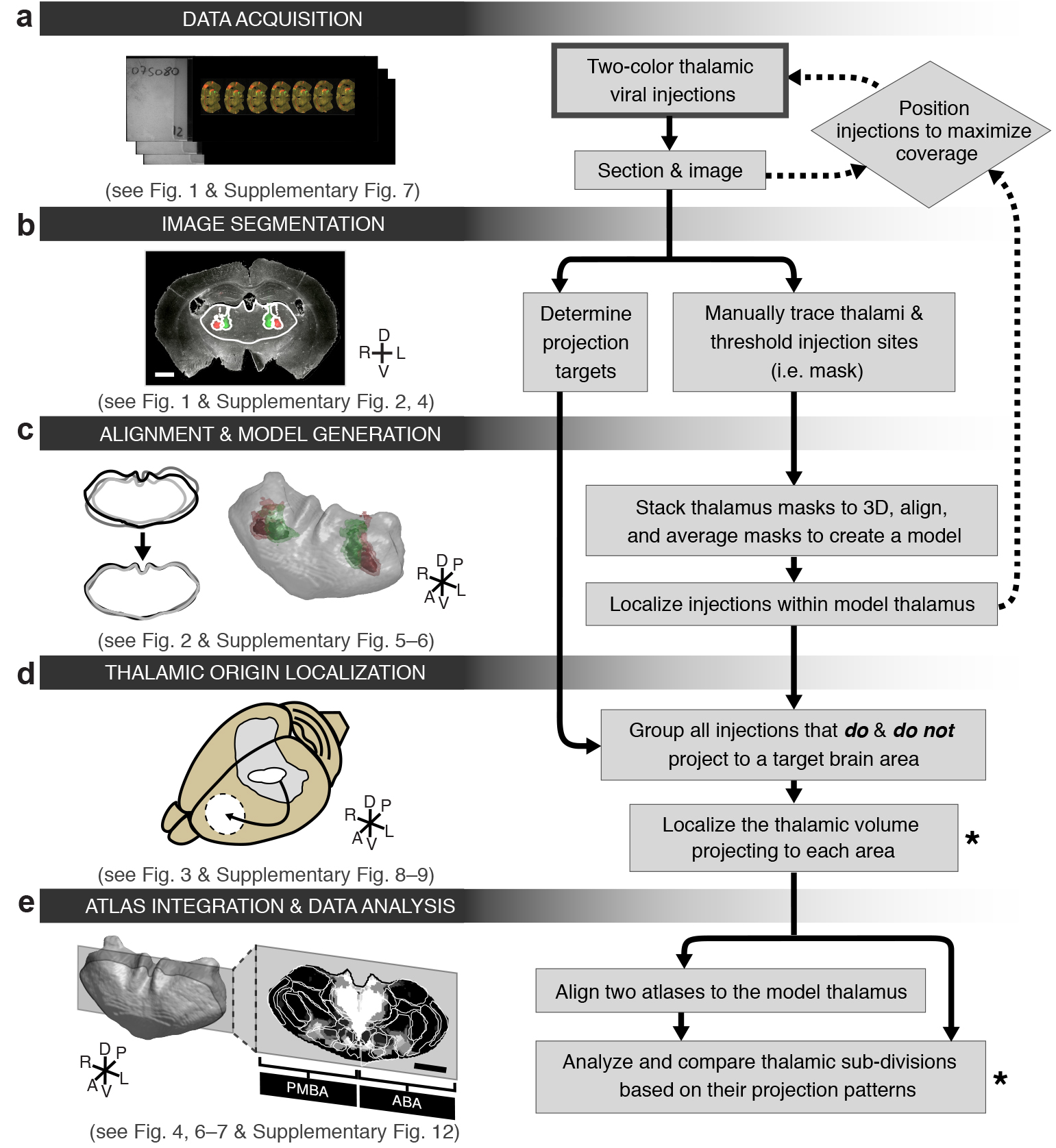
Schematic flow chart of anatomical tracing and analysis methods. (a) Data acquisition: the entire thalamus is labeled with small viral injections, sectioned, and imaged at a 0.5 μm/pixel resolution. (b) Image segmentation and projection identification: binary masks of the thalamus and injection sites are created and cortical sub-regions are scored for the presence or absence of projections. (c) Data alignment and model generation: thalamus masks are rotated, sheared, scaled and aligned. The aligned masks are then averaged to create a model thalamus. All injection sites are subsequently mapped onto the model thalamus. (d) Thalamic origin localization: injection site location and projection information are combined to define the precise thalamic volume projecting to a region of interest. (e) Atlas integration and data analysis: thalamic output patterns are determined using either the classic nuclear subdivision of the Paxinos Mouse Brain Atlas (PMBA) and the Allen Brain Atlas (ABA), or through atlas independent projection analyses. The thick-lined box indicates the starting point of the experiment while asterisks indicate the major output of the data analysis. All scale bars are 1 mm.
3D rendering of the thalami and corresponding viral injections of all 75 experimental brains. Each row shows an oblique, dorsal, anterior, and lateral view of an individual experimental thalamus. Axis descriptions are shown for the first thalamus only. Viral injection sites (red/green fluorescence) are shown within the traced thalamus from each brain (gray). A darker center of each injection site represents the eroded ‘core’ of the injection as described in Figure 1.
Slice angle estimation from anatomical landmark positions. Slice angle is estimated using the slice locations of several landmarks. In each case, the landmarks form a triangle, either between the medial anterior corpus callosum (aCC), the anterior commissure (AC) and the anterior dentate gyrus (DG) (i = 1, red) or between the aCC, the AC, and the medial posterior corpus callosum (pCC) (i = 2, blue). Assuming the sides of the triangle are fixed and proportional to the atlas dimensions (ABA), we can define the angles γ1 and γ2, using the red and blue coordinates, respectively. The fixed sides of the red triangle constrain the relationship between zA1 and zB1 so that θ1 (estimated cutting angle) can be found from slice locations zA1 and zB1 only (and similarly for θ2). θ1 and θ2 were determined from the equation numerically, and the final cutting angle tilt estimation was the average of θ1 and θ2. Baseline θABA values for ABA sections were measured from ABA landmark locations, and brains with |θC− θABA| > 2° were subjected to rotation correction.
Variability across thalamus masks and cytoarchitecturally identifiable thalamic structures. (a) 3D rendering of the model thalamus created by averaging individual thalamus masks (oblique view). (b) To assess thalamus mask variability, we created the 3D perimeter matrix P, which contains the sum of the perimeter voxels of all 75 experimental thalamus masks. Color map indicates the summed projection of P along dorsal-ventral axis. (c) The top panels show x-y cross sections through P at the z locations marked in panel b as 1, 2, and 3. The bottom panels show profiles at the locations indicated in top of each panel (white lines). Full width half maximum (FWHM) across all profiles is 102 ± 51 μm (mean ± s.d.). (d) Histogram of Dice’s Similarity Coefficient for individual thalamus masks. Individual thalamus masks are highly similar to the model thalamus, with Dice’s coefficient between individual masks and the model D = 0.94 ± 0.01 (mean ± s.d.). (e) Four cytoarchitecturally identifiable thalamic structures (AD, AV, PT, and fr) were manually traced in five experimental brains and two atlases (PMBA and ABA), as described in Figure 2b–c. Dice’s Similarity Coefficient is plotted to compare the identified structures in two separate atlases (left, n = 2), to compare the atlases to the experimentally traced structures (middle, n = 5, mean ± s.d.), and to compare the experimentally traced structures to each other (right, n = 10, mean ± s.d.). All scale bars are 1 mm.
Full characterization of injection coverage within the model thalamus. (a) Oblique view of the model thalamus (gray) with the center of mass of all 254 injection sites (black crosses). (b) Coverage of the thalamus broken down by nucleus. Fraction of each nucleus covered by at least 1, and at least 2, at least 4, at least 6 and at least 10 injections, showing that the entire volume of most thalamic nuclei is sampled at least 4 times. (c) Full coverage montage of the thalamus. Coronal slices through the thalamus starting at −0.155 mm posterior to bregma, and continuing in 50 μm increments to the posterior end of the thalamus. The color scale indicates the number of times an independent injection labeled a given location of the thalamus.
Projection scoring criteria and injection grouping method. (a) PMBA sections with corresponding mouse brain images on the right, showing example projection distributions within several regions of interest (ROIs) in the frontal cortex. (b) Diagram of projection scoring criteria: strength (either dense or sparse labeling within the ROI) and specificity (either projections locally confined to the ROI or projections that also go to surrounding areas). Partial or full coverage within the ROI was also scored, but differences in thalamic origin profiles were not found (data not shown). (c) Description of each binary mask created by grouping the scored injections as described. (d) Example confidence map created by summing the binary masks created in c, where each mask adds a value of 1, and all masks (A–H) must be true at a given point to reach a confidence level of 8 (white). (e–g) Illustration of how a confidence map is created. (e) Illustration of eight injections and their corresponding score, showing the full injection as well as the eroded core. (f) Sample of the binary masks created from panel e as described in panel c. (g) Confidence map created from panel f as described in panel d. All scale bars are 1 mm.
Full confidence maps for the thalamic origin of all cortical projections. (a) The cortical areas examined (modified from PMBA25 and reference 47) are shown. Lateral and medial whole brain views (top) and coronal sections from anterior to posterior (bottom). (b) Reference coronal sections for the confidence maps shown in panel c, with the bregma coordinates noted in the anterior-posterior axis. (c) Each column contains the confidence map for a given cortical sub-region, arranged alphabetically, with coronal sections corresponding to those in panel b. The confidence maps (gray scale) show the thalamic origin of projections to nineteen cortical sub-regions: FrA, LO, VO, MO, IL, PrL, vACC, dACC, RS, Pt, M2, M1, S1/2, AI, Ins, Rhi, Tem, Vis, and Aud. The outline of the model thalamus is shown in white for each section, and the aligned nuclei from PMBA (left) and the ABA (right), are overlaid as colored outlines (nuclei labeled for AI only). All scale bars are 1 mm.
Retrograde bead injections fall within the thalamic volume predicted by the confidence maps. (a) Reference coronal sections for the confidence maps shown in panel b–d, with the bregma coordinates noted in the anterior-posterior axis. (b–d) Thalamic location of retrogradely transported beads 3 days after injection in the indicated cortical sub-region (total of 10 mice injected and 3 analyzed in detail). The confidence maps (gray scale, left: see Fig. 3 for detail) show the predicted thalamic origin of projections to three cortical sub-regions; (b) IL, (c) PrL, and (d) vM1. The locations of beads that were retrogradely transported from the indicated cortical region are overlaid on the left of each confidence map section (red dots), and shown independently on the right. The outline of the model thalamus is shown for each section (left: white, right: black). All scale bars are 1 mm.
Optimal injection coordinates used to target specific thalamocortical projections. Optimal injection coordinates, i.e. the most probable location to inject in order to target a specific thalamocortical pathway, were determined for each of the 19 cortical subregions: FrA, LO, VO, MO, IL, PrL, vACC, dACC, RS, Pt, M2, M1, S1/2, AI, Ins, Rhi, Tem, Vis, and Aud. The orientation of each thalamus view is indicated in the top left column. The colored areas for each cortical projection sub-region denote the location with the highest probability to label those projections. A single set of coordinates is listed to the right of each cortical sub-region. All coordinates are shown in millimeters relative to bregma.
Nuclear localization of the thalamic origins of cortical projections. (a) The fractions of each thalamic nucleus projecting to Aud, dACC, Ins, M1, M2, MO, Pt, PrL, Rhi, RS, S1/2, Tem, vACC, Vis, and VO are shown in three confidence levels (dashed lines) with their average (black line). Vertical gray line: the inflection point in the color scale used in panel b. (b) Spatial representations of all nuclei projecting to the each cortical sub-region, arranged alphabetically. Circle diameters correspond to the relative size of each nucleus and their positions correspond to their relative center-of-mass location within the thalamus in the anterior-posterior and medial-lateral axes. Auditory cortex is not shown because we did not identify any projections from our injections.
Localizing and verifying the thalamic nuclear origins of cortical projections. (a) Comparison of our thalamic nuclear localization data in mouse to previous studies of thalamocortical projections in the adult rat. Nuclear localization map as described in Figure 6e, overlaid with the PubMed ID #’s for publications with evidence for the corresponding thalamocortical projection. Some specific projections are inferred from data presented in the publications. Asterisks indicate thalamic nuclei with little or no anatomical data in the rat literature. (b) Examples of several atlases used in literature to classify cortical sub-regions in the literature. (c) Comparison of nuclear localization maps for two atlases separately (ABA and PMBA). Left: Coronal section showing the nuclear subdivisions from the PMBA (left) and ABA (right). Nucleus colors indicate the fraction of each nucleus covered by the dACC confidence map described in Figure 6. Right: Aggregate nucleus coverage map of all thalamocortical projections using the PMBA and ABA separately. Nuclei (rows) and cortical sub-regions (columns) are ordered as in Figure 6e. The ABA and PMBA specific maps were averaged to produce Figure 6e. (d) Comparison of nuclear localization maps for separate confidence levels (using averaged atlases). Left: The fraction of each nucleus projecting to AI, shown for three confidence levels (dashed lines, 3, 5 and 7) and their average (black line) as described in Figure 6. Right: Nucleus localization maps for the three confidence levels. Nuclei (rows) and cortical sub-regions (columns) are ordered as in Figure 6e. All three maps are averaged to produce Figure 6e.
vM1 layer boundaries and background fluorescence. (a) Representative vM1 image showing the layer boundaries. Relative thicknesses of cortical layers in vM1 vary from the lateral edge to the medial edge. The parameters used in calculations are indicated: l: relative cortical depth (0 at the pia and 1 at white matter); θ: the angel of the ROI. Horizontal lines: layer boundaries. The depth regions analyzed for layer preferential projections are indicated (color bars). (b) Schematic of layer depth variation from medial to lateral edge. The boundaries at the medial and lateral edges are based on previous characterizations. At other radial positions, the layer boundaries were linearly interpolated from the lateral to medial edges. The boundaries were normalized to the cortical layer depth. Colored regions and lines indicate the regions analyzed for layer preferential projections. (c) Background florescence along the normalized cortical depth. All fluorescence was first mapped to the corresponding layer depth at the medial edge before being binned and averaged. Background fluorescence was calculated as the median fluorescence at a depth bin across brains manually determined not to have projections from the thalamus to vM1. (d) Assessment of 11 thalamic voxel clusters’ layer-preferential projections to vM1. The clusters were determined as described in Figure 4. The occupied fraction of each thalamic voxel cluster containing layer-preferential projections to L2/3–5a (cyan) or 5b (magenta) of vM1 is plotted as a fraction of total cluster volume.
Acknowledgments
We thank Dr. Karel Svoboda and HHMI, Janelia Farm Research Campus for their generous support in the initiation and data collection phase of this project. All Nanozoomer imaging were collected in Janelia Farm Research Campus. We thank Dr. Claudio Mello, Maozhen Qin, Dr. Jian Qiu, Jessica Li, Dr. Stefanie Kaech Petrie, Anthony Gilmore, Dr. Yi Zuo, and Dr. Daniel Lioy for technical support. We thank Drs. Karel Svoboda, Jeff Lichtman, Kun Huang and Bo Li for their discussions and Drs. Karel Svoboda, John Williams, and John Adelman for comments on the manuscript. We thank Robin Champieux and Kyle Banerjee for establishing web data depository. We also thank the anonymous reviewers who gave some critical suggestions that helped us to improve the data analysis, presentation and depository. This work is supported by an ARRA P30 grant (PI: Dr. Richard Goodman), an NSF-GRF fellowship (BJH), ARCS Foundation Portland Chapter (BJH), an NIH Director’s Innovator Award (HZ), an NIH R01 grant (NS081071; TM), and the Medical Research Foundation (TM).
Footnotes
Author Contributions:
All authors participated in designing the experiments. BJH, DK, KJG, and TM performed the experiments, BJH, BRL, KJG, DK, HZ and TM analyzed the data. BJH, BRL, KJG, HZ and TM wrote the manuscript.
The authors declare no competing financial interests.
The raw data and the analyzed data are publicly available at http://digitalcollections.ohsu.edu/projectionmap. The original resolution images are available upon request as hard drive format.
A supplementary methods checklist is available.
References
- 1.Bohland JW, et al. A Proposal for a Coordinated Effort for the Determination of Brainwide Neuroanatomical Connectivity in Model Organisms at a Mesoscopic Scale. PLoS Comput Biol. 2009;5:e1000334. doi: 10.1371/journal.pcbi.1000334. [DOI] [PMC free article] [PubMed] [Google Scholar]
- 2.Luo L, Callaway EM, Svoboda K. Genetic dissection of neural circuits. Neuron. 2008;57:634–660. doi: 10.1016/j.neuron.2008.01.002. [DOI] [PMC free article] [PubMed] [Google Scholar]
- 3.Lichtman JW, Denk W. The big and the small: challenges of imaging the brain’s circuits. Science. 2011;334:618–623. doi: 10.1126/science.1209168. [DOI] [PubMed] [Google Scholar]
- 4.Jones EG. The Thalamus 2 Volume Set. Cambridge University Press; 2007. [Google Scholar]
- 5.Sherman SM, Guillery RW. Exploring the Thalamus and Its Role in Cortical Function. MIT Press (MA); 2009. [Google Scholar]
- 6.Groenewegen HJ, Berendse HW, Wolters JG, Lohman AH. The anatomical relationship of the prefrontal cortex with the striatopallidal system, the thalamus and the amygdala: evidence for a parallel organization. Prog Brain Res. 1990;85:95–116. doi: 10.1016/s0079-6123(08)62677-1. discussion 116–8. [DOI] [PubMed] [Google Scholar]
- 7.Evarts EV, Thach WT. Motor mechanisms of the CNS: cerebrocerebellar interrelations. Annu Rev Physiol. 1969;31:451–498. doi: 10.1146/annurev.ph.31.030169.002315. [DOI] [PubMed] [Google Scholar]
- 8.Steriade M, Llinás RR. The functional states of the thalamus and the associated neuronal interplay. Physiological Reviews. 1988;68:649–742. doi: 10.1152/physrev.1988.68.3.649. [DOI] [PubMed] [Google Scholar]
- 9.Asanuma H, Fernandez JJ. Organization of projection from the thalamic relay nuclei to the motor cortex in the cat. Brain Res. 1974;71:515–522. doi: 10.1016/0006-8993(74)90995-0. [DOI] [PubMed] [Google Scholar]
- 10.Nauta WJ. The problem of the frontal lobe: a reinterpretation. J Psychiatr Res. 1971;8:167–187. doi: 10.1016/0022-3956(71)90017-3. [DOI] [PubMed] [Google Scholar]
- 11.Kolb B. Studies on the caudate-putamen and the dorsomedial thalamic nucleus of the rat: implications for mammalian frontal-lobe functions. Physiology & Behavior. 1977;18:237–244. doi: 10.1016/0031-9384(77)90128-7. [DOI] [PubMed] [Google Scholar]
- 12.Weinberger DR. A connectionist approach to the prefrontal cortex. J Neuropsychiatry Clin Neurosci. 1993;5:241–253. doi: 10.1176/jnp.5.3.241. [DOI] [PubMed] [Google Scholar]
- 13.Berman AL, Jones EG. The Thalamus and Basal Telencephalon of the Cat. 1982 [Google Scholar]
- 14.Walker AE. The Primate Thalamus. University of Chicago Press; 1938. [Google Scholar]
- 15.Bota M, Dong HW, Swanson LW. Combining collation and annotation efforts toward completion of the rat and mouse connectomes in BAMS. Frontiers in neuroinformatics. 2012 doi: 10.3389/fninf.2012.00002. [DOI] [PMC free article] [PubMed] [Google Scholar]
- 16.Mao T, et al. Long-range neuronal circuits underlying the interaction between sensory and motor cortex. Neuron. 2011;72:111–123. doi: 10.1016/j.neuron.2011.07.029. [DOI] [PMC free article] [PubMed] [Google Scholar]
- 17.Harris JA, Oh SW, Zeng H. Adeno Associated Viral Vectors for Anterograde Axonal Tracing with Fluorescent Proteins in Nontransgenic and Cre Driver Mice. Current protocols. 2012 doi: 10.1002/0471142301.ns0120s59. [DOI] [PubMed] [Google Scholar]
- 18.McFarland NR, Lee JS, Hyman BT, McLean PJ. Comparison of transduction efficiency of recombinant AAV serotypes 1, 2, 5, and 8 in the rat nigrostriatal system. Journal of Neurochemistry. 2009;109:838–845. doi: 10.1111/j.1471-4159.2009.06010.x. [DOI] [PMC free article] [PubMed] [Google Scholar]
- 19.Aschauer DF, Kreuz S, Rumpel S. Analysis of transduction efficiency, tropism and axonal transport of AAV serotypes 1, 2, 5, 6, 8 and 9 in the mouse brain. PLoS ONE. 2013;8:e76310. doi: 10.1371/journal.pone.0076310. [DOI] [PMC free article] [PubMed] [Google Scholar]
- 20.Hoover WB, Vertes RP. Anatomical analysis of afferent projections to the medial prefrontal cortex in the rat. Brain Struct Funct. 2007;212:149–179. doi: 10.1007/s00429-007-0150-4. [DOI] [PubMed] [Google Scholar]
- 21.Wang Q, Burkhalter A. Area map of mouse visual cortex. J Comp Neurol. 2007;502:339–357. doi: 10.1002/cne.21286. [DOI] [PubMed] [Google Scholar]
- 22.Thompson RH, Swanson LW. Hypothesis-driven structural connectivity analysis supports network over hierarchical model of brain architecture. Proceedings of the National Academy of Sciences. 2010;107:15235–15239. doi: 10.1073/pnas.1009112107. [DOI] [PMC free article] [PubMed] [Google Scholar]
- 23.Otsu N. A threshold selection method from gray-level histograms. Automatica. 1975 [Google Scholar]
- 24.Ragan T, et al. Serial two-photon tomography for automated ex vivo mouse brain imaging. Nat Meth. 2012;9:255–258. doi: 10.1038/nmeth.1854. [DOI] [PMC free article] [PubMed] [Google Scholar]
- 25.Paxinos G. The mouse brain in stereotaxic coordinates. 2004 [Google Scholar]
- 26.Knapska E, Marcias M, Mikosz M. Functional anatomy of neural circuits regulating fear and extinction. Proceedings of the National Academy of Sciences. 2012;42:1–6. doi: 10.1073/pnas.1202087109. [DOI] [PMC free article] [PubMed] [Google Scholar]
- 27.Dantzker JL, Callaway EM. Laminar sources of synaptic input to cortical inhibitory interneurons and pyramidal neurons. Nat Neurosci. 2000;3:701–707. doi: 10.1038/76656. [DOI] [PubMed] [Google Scholar]
- 28.Shepherd GMG, Stepanyants A, Bureau I, Chklovskii D, Svoboda K. Geometric and functional organization of cortical circuits. Nat Neurosci. 2005;8:782–790. doi: 10.1038/nn1447. [DOI] [PubMed] [Google Scholar]
- 29.Groenewegen HJ. Organization of the afferent connections of the mediodorsal thalamic nucleus in the rat, related to the mediodorsal-prefrontal topography. NSC. 1988;24:379–431. doi: 10.1016/0306-4522(88)90339-9. [DOI] [PubMed] [Google Scholar]
- 30.Ray JP, Price JL. The organization of the thalamocortical connections of the mediodorsal thalamic nucleus in the rat, related to the ventral forebrain-prefrontal cortex topography. J Comp Neurol. 1992;323:167–197. doi: 10.1002/cne.903230204. [DOI] [PubMed] [Google Scholar]
- 31.Lein ES, et al. Genome-wide atlas of gene expression in the adult mouse brain. Nature. 2007;445:168–176. doi: 10.1038/nature05453. [DOI] [PubMed] [Google Scholar]
- 32.Haque T, et al. Thalamic afferent and efferent connectivity to cerebral cortical areas with direct projections to identified subgroups of trigeminal premotoneurons in the rat. Brain Res. 2010;1346:69–82. doi: 10.1016/j.brainres.2010.05.034. [DOI] [PubMed] [Google Scholar]
- 33.Desbois C, Villanueva L. The organization of lateral ventromedial thalamic connections in the rat: a link for the distribution of nociceptive signals to widespread cortical regions. NSC. 2001;102:885–898. doi: 10.1016/s0306-4522(00)00537-6. [DOI] [PubMed] [Google Scholar]
- 34.Berendse HW, Groenewegen HJ. Restricted cortical termination fields of the midline and intralaminar thalamic nuclei in the rat. NSC. 1991;42:73–102. doi: 10.1016/0306-4522(91)90151-d. [DOI] [PubMed] [Google Scholar]
- 35.Vertes RP, Hoover WB, Rodriguez JJ. Projections of the central medial nucleus of the thalamus in the rat: node in cortical, striatal and limbic forebrain circuitry. Neuroscience. 2012;219:120–136. doi: 10.1016/j.neuroscience.2012.04.067. [DOI] [PubMed] [Google Scholar]
- 36.Van der Werf YD, Witter MP, Groenewegen HJ. The intralaminar and midline nuclei of the thalamus. Anatomical and functional evidence for participation in processes of arousal and awareness. Brain Res Brain Res Rev. 2002;39:107–140. doi: 10.1016/s0165-0173(02)00181-9. [DOI] [PubMed] [Google Scholar]
- 37.Hooks BM, et al. Organization of cortical and thalamic input to pyramidal neurons in mouse motor cortex. Journal of Neuroscience. 2013;33:748–760. doi: 10.1523/JNEUROSCI.4338-12.2013. [DOI] [PMC free article] [PubMed] [Google Scholar]
- 38.Hintiryan H, et al. Comprehensive connectivity of the mouse main olfactory bulb: analysis and online digital atlas. Front Neuroanat. 2012;6:1–16. doi: 10.3389/fnana.2012.00030. [DOI] [PMC free article] [PubMed] [Google Scholar]
- 39.Oh SW, et al. A mesoscale connectome of the mouse brain. Nature. 2014:1–21. doi: 10.1038/nature13186. [DOI] [PMC free article] [PubMed] [Google Scholar]
- 40.Zingg B, et al. Neural Networks of the Mouse Neocortex. Cell. 2014;156:1096–1111. doi: 10.1016/j.cell.2014.02.023. [DOI] [PMC free article] [PubMed] [Google Scholar]
- 41.Spear LP. The adolescent brain and age-related behavioral manifestations. Neurosci Biobehav Rev. 2000;24:417–463. doi: 10.1016/s0149-7634(00)00014-2. [DOI] [PubMed] [Google Scholar]
- 42.Van Eden CG, Uylings HB. Postnatal volumetric development of the prefrontal cortex in the rat. J Comp Neurol. 1985;241:268–274. doi: 10.1002/cne.902410303. [DOI] [PubMed] [Google Scholar]
- 43.CASEY BJ, Getz S, Galvan A. The adolescent brain. Dev Rev. 2008;28:62–77. doi: 10.1016/j.dr.2007.08.003. [DOI] [PMC free article] [PubMed] [Google Scholar]
- 44.Kolmac CI, Mitrofanis J. Organisation of the reticular thalamic projection to the intralaminar and midline nuclei in rats. J Comp Neurol. 1997;377:165–178. doi: 10.1002/(sici)1096-9861(19970113)377:2<165::aid-cne2>3.0.co;2-1. [DOI] [PubMed] [Google Scholar]
- 45.Dice LR. Convergent inputs from electrically and topographically distinct orexin cells to locus coeruleus and ventral tegmental area. Ecology. 1945 doi: 10.1111/j.1460-9568.2012.08057.x. [DOI] [PMC free article] [PubMed] [Google Scholar]
- 46.Petreanu L, Mao T, Sternson SM, Svoboda K. The subcellular organization of neocortical excitatory connections. Nature. 2009;457:1142–1145. doi: 10.1038/nature07709. [DOI] [PMC free article] [PubMed] [Google Scholar]
- 47.Watson C, Paxinos G, Puelles L. The Mouse Nervous System. Academic Press; 2012. [Google Scholar]
Associated Data
This section collects any data citations, data availability statements, or supplementary materials included in this article.
Supplementary Materials
Full confidence maps as 3D stacks for AI, LO, VO, MO, IL, PrL, vACC, dACC, FrA, respectively. Distance from bregma for each section is indicated. All scale bars are 1 mm.
Characterization of viral injections. (a) Dorsal view of a mouse brain (dashed white outline) after receiving a large, unilateral thalamic injection (~100 nL); demonstrating that thalamic projections do not cross the midline in mouse. (b–c) Representative confocal image at the center of a thalamic injection site showing all cell nuclei (DAPI, blue), neurons (NeuN, red), and virally labeled cells (eGFP, green), shown individually in b, and overlaid in c. (d) The fraction of total cells infected at the center of an injection site (n = 17 green bar, mean ± s.d.). The fraction of total cells that are neurons at the center of an injection site (n = 5: red bar, mean ± s.d.). (e) The fraction of neurons infected at the center of an injection site (n = 5: yellow bar, mean ± s.d.). (f–g) Representative confocal image at the center of a thalamic co-injection of two viruses showing all cell nuclei (DAPI, blue), cells infected by virus expressing the fluorophore tdTomato (red), and cells infected by virus expressing the fluorophore eGFP (green), shown individually in f, and overlaid in g. (h) Quantification of the fraction of total cells expressing one or both co-injected viruses, showing that total infectable cell population is larger than a single injection will infect on average (n = 4, mean ± s. d.). All scale bars are 50 μm.
Two-color injections reveal topographic projection information. (a) Illustration showing the section locations for images in b and c. (b–c) Example thalamus sections showing injection sites (bottom), and example cortical sections showing thalamocortical projections (top). The insets for b and c show a zoomed image of juxtaposed red and green projections. (b) The green injection in the right hemisphere projects to AI, while the red injection, which originated lateral to the green injection in the thalamus, sends axonal projections to more medial brain structures, including LO, which is immediately adjacent to AI. (c) The green injection in the left hemisphere projects primarily to cortical layers 1 and 2/3 in the cingulate cortex, while the red injection projects to all cortical layers of motor cortex immediately adjacent to the green projections, largely maintaining separation of their respective projection fields. All scale bars are 1 mm unless otherwise specified.
Schematic flow chart of anatomical tracing and analysis methods. (a) Data acquisition: the entire thalamus is labeled with small viral injections, sectioned, and imaged at a 0.5 μm/pixel resolution. (b) Image segmentation and projection identification: binary masks of the thalamus and injection sites are created and cortical sub-regions are scored for the presence or absence of projections. (c) Data alignment and model generation: thalamus masks are rotated, sheared, scaled and aligned. The aligned masks are then averaged to create a model thalamus. All injection sites are subsequently mapped onto the model thalamus. (d) Thalamic origin localization: injection site location and projection information are combined to define the precise thalamic volume projecting to a region of interest. (e) Atlas integration and data analysis: thalamic output patterns are determined using either the classic nuclear subdivision of the Paxinos Mouse Brain Atlas (PMBA) and the Allen Brain Atlas (ABA), or through atlas independent projection analyses. The thick-lined box indicates the starting point of the experiment while asterisks indicate the major output of the data analysis. All scale bars are 1 mm.
3D rendering of the thalami and corresponding viral injections of all 75 experimental brains. Each row shows an oblique, dorsal, anterior, and lateral view of an individual experimental thalamus. Axis descriptions are shown for the first thalamus only. Viral injection sites (red/green fluorescence) are shown within the traced thalamus from each brain (gray). A darker center of each injection site represents the eroded ‘core’ of the injection as described in Figure 1.
Slice angle estimation from anatomical landmark positions. Slice angle is estimated using the slice locations of several landmarks. In each case, the landmarks form a triangle, either between the medial anterior corpus callosum (aCC), the anterior commissure (AC) and the anterior dentate gyrus (DG) (i = 1, red) or between the aCC, the AC, and the medial posterior corpus callosum (pCC) (i = 2, blue). Assuming the sides of the triangle are fixed and proportional to the atlas dimensions (ABA), we can define the angles γ1 and γ2, using the red and blue coordinates, respectively. The fixed sides of the red triangle constrain the relationship between zA1 and zB1 so that θ1 (estimated cutting angle) can be found from slice locations zA1 and zB1 only (and similarly for θ2). θ1 and θ2 were determined from the equation numerically, and the final cutting angle tilt estimation was the average of θ1 and θ2. Baseline θABA values for ABA sections were measured from ABA landmark locations, and brains with |θC− θABA| > 2° were subjected to rotation correction.
Variability across thalamus masks and cytoarchitecturally identifiable thalamic structures. (a) 3D rendering of the model thalamus created by averaging individual thalamus masks (oblique view). (b) To assess thalamus mask variability, we created the 3D perimeter matrix P, which contains the sum of the perimeter voxels of all 75 experimental thalamus masks. Color map indicates the summed projection of P along dorsal-ventral axis. (c) The top panels show x-y cross sections through P at the z locations marked in panel b as 1, 2, and 3. The bottom panels show profiles at the locations indicated in top of each panel (white lines). Full width half maximum (FWHM) across all profiles is 102 ± 51 μm (mean ± s.d.). (d) Histogram of Dice’s Similarity Coefficient for individual thalamus masks. Individual thalamus masks are highly similar to the model thalamus, with Dice’s coefficient between individual masks and the model D = 0.94 ± 0.01 (mean ± s.d.). (e) Four cytoarchitecturally identifiable thalamic structures (AD, AV, PT, and fr) were manually traced in five experimental brains and two atlases (PMBA and ABA), as described in Figure 2b–c. Dice’s Similarity Coefficient is plotted to compare the identified structures in two separate atlases (left, n = 2), to compare the atlases to the experimentally traced structures (middle, n = 5, mean ± s.d.), and to compare the experimentally traced structures to each other (right, n = 10, mean ± s.d.). All scale bars are 1 mm.
Full characterization of injection coverage within the model thalamus. (a) Oblique view of the model thalamus (gray) with the center of mass of all 254 injection sites (black crosses). (b) Coverage of the thalamus broken down by nucleus. Fraction of each nucleus covered by at least 1, and at least 2, at least 4, at least 6 and at least 10 injections, showing that the entire volume of most thalamic nuclei is sampled at least 4 times. (c) Full coverage montage of the thalamus. Coronal slices through the thalamus starting at −0.155 mm posterior to bregma, and continuing in 50 μm increments to the posterior end of the thalamus. The color scale indicates the number of times an independent injection labeled a given location of the thalamus.
Projection scoring criteria and injection grouping method. (a) PMBA sections with corresponding mouse brain images on the right, showing example projection distributions within several regions of interest (ROIs) in the frontal cortex. (b) Diagram of projection scoring criteria: strength (either dense or sparse labeling within the ROI) and specificity (either projections locally confined to the ROI or projections that also go to surrounding areas). Partial or full coverage within the ROI was also scored, but differences in thalamic origin profiles were not found (data not shown). (c) Description of each binary mask created by grouping the scored injections as described. (d) Example confidence map created by summing the binary masks created in c, where each mask adds a value of 1, and all masks (A–H) must be true at a given point to reach a confidence level of 8 (white). (e–g) Illustration of how a confidence map is created. (e) Illustration of eight injections and their corresponding score, showing the full injection as well as the eroded core. (f) Sample of the binary masks created from panel e as described in panel c. (g) Confidence map created from panel f as described in panel d. All scale bars are 1 mm.
Full confidence maps for the thalamic origin of all cortical projections. (a) The cortical areas examined (modified from PMBA25 and reference 47) are shown. Lateral and medial whole brain views (top) and coronal sections from anterior to posterior (bottom). (b) Reference coronal sections for the confidence maps shown in panel c, with the bregma coordinates noted in the anterior-posterior axis. (c) Each column contains the confidence map for a given cortical sub-region, arranged alphabetically, with coronal sections corresponding to those in panel b. The confidence maps (gray scale) show the thalamic origin of projections to nineteen cortical sub-regions: FrA, LO, VO, MO, IL, PrL, vACC, dACC, RS, Pt, M2, M1, S1/2, AI, Ins, Rhi, Tem, Vis, and Aud. The outline of the model thalamus is shown in white for each section, and the aligned nuclei from PMBA (left) and the ABA (right), are overlaid as colored outlines (nuclei labeled for AI only). All scale bars are 1 mm.
Retrograde bead injections fall within the thalamic volume predicted by the confidence maps. (a) Reference coronal sections for the confidence maps shown in panel b–d, with the bregma coordinates noted in the anterior-posterior axis. (b–d) Thalamic location of retrogradely transported beads 3 days after injection in the indicated cortical sub-region (total of 10 mice injected and 3 analyzed in detail). The confidence maps (gray scale, left: see Fig. 3 for detail) show the predicted thalamic origin of projections to three cortical sub-regions; (b) IL, (c) PrL, and (d) vM1. The locations of beads that were retrogradely transported from the indicated cortical region are overlaid on the left of each confidence map section (red dots), and shown independently on the right. The outline of the model thalamus is shown for each section (left: white, right: black). All scale bars are 1 mm.
Optimal injection coordinates used to target specific thalamocortical projections. Optimal injection coordinates, i.e. the most probable location to inject in order to target a specific thalamocortical pathway, were determined for each of the 19 cortical subregions: FrA, LO, VO, MO, IL, PrL, vACC, dACC, RS, Pt, M2, M1, S1/2, AI, Ins, Rhi, Tem, Vis, and Aud. The orientation of each thalamus view is indicated in the top left column. The colored areas for each cortical projection sub-region denote the location with the highest probability to label those projections. A single set of coordinates is listed to the right of each cortical sub-region. All coordinates are shown in millimeters relative to bregma.
Nuclear localization of the thalamic origins of cortical projections. (a) The fractions of each thalamic nucleus projecting to Aud, dACC, Ins, M1, M2, MO, Pt, PrL, Rhi, RS, S1/2, Tem, vACC, Vis, and VO are shown in three confidence levels (dashed lines) with their average (black line). Vertical gray line: the inflection point in the color scale used in panel b. (b) Spatial representations of all nuclei projecting to the each cortical sub-region, arranged alphabetically. Circle diameters correspond to the relative size of each nucleus and their positions correspond to their relative center-of-mass location within the thalamus in the anterior-posterior and medial-lateral axes. Auditory cortex is not shown because we did not identify any projections from our injections.
Localizing and verifying the thalamic nuclear origins of cortical projections. (a) Comparison of our thalamic nuclear localization data in mouse to previous studies of thalamocortical projections in the adult rat. Nuclear localization map as described in Figure 6e, overlaid with the PubMed ID #’s for publications with evidence for the corresponding thalamocortical projection. Some specific projections are inferred from data presented in the publications. Asterisks indicate thalamic nuclei with little or no anatomical data in the rat literature. (b) Examples of several atlases used in literature to classify cortical sub-regions in the literature. (c) Comparison of nuclear localization maps for two atlases separately (ABA and PMBA). Left: Coronal section showing the nuclear subdivisions from the PMBA (left) and ABA (right). Nucleus colors indicate the fraction of each nucleus covered by the dACC confidence map described in Figure 6. Right: Aggregate nucleus coverage map of all thalamocortical projections using the PMBA and ABA separately. Nuclei (rows) and cortical sub-regions (columns) are ordered as in Figure 6e. The ABA and PMBA specific maps were averaged to produce Figure 6e. (d) Comparison of nuclear localization maps for separate confidence levels (using averaged atlases). Left: The fraction of each nucleus projecting to AI, shown for three confidence levels (dashed lines, 3, 5 and 7) and their average (black line) as described in Figure 6. Right: Nucleus localization maps for the three confidence levels. Nuclei (rows) and cortical sub-regions (columns) are ordered as in Figure 6e. All three maps are averaged to produce Figure 6e.
vM1 layer boundaries and background fluorescence. (a) Representative vM1 image showing the layer boundaries. Relative thicknesses of cortical layers in vM1 vary from the lateral edge to the medial edge. The parameters used in calculations are indicated: l: relative cortical depth (0 at the pia and 1 at white matter); θ: the angel of the ROI. Horizontal lines: layer boundaries. The depth regions analyzed for layer preferential projections are indicated (color bars). (b) Schematic of layer depth variation from medial to lateral edge. The boundaries at the medial and lateral edges are based on previous characterizations. At other radial positions, the layer boundaries were linearly interpolated from the lateral to medial edges. The boundaries were normalized to the cortical layer depth. Colored regions and lines indicate the regions analyzed for layer preferential projections. (c) Background florescence along the normalized cortical depth. All fluorescence was first mapped to the corresponding layer depth at the medial edge before being binned and averaged. Background fluorescence was calculated as the median fluorescence at a depth bin across brains manually determined not to have projections from the thalamus to vM1. (d) Assessment of 11 thalamic voxel clusters’ layer-preferential projections to vM1. The clusters were determined as described in Figure 4. The occupied fraction of each thalamic voxel cluster containing layer-preferential projections to L2/3–5a (cyan) or 5b (magenta) of vM1 is plotted as a fraction of total cluster volume.