

Abstract
Time-integrated fluorescence cumulant analysis (TIFCA) is a data analysis technique for fluorescence fluctuation spectroscopy (FFS) that extracts information from the cumulants of the integrated fluorescence intensity. It is the first exact theory that describes the effect of sampling time on FFS experiment. Rebinning of data to longer sampling times helps to increase the signal/noise ratio of the experimental cumulants of the photon counts. The sampling time dependence of the cumulants encodes both brightness and diffusion information of the sample. TIFCA analysis extracts this formation by fitting the cumulants to model functions. Generalization of TIFCA to multicolor FFS experiment is straightforward. Here, we present an overview of the theory, its implementation, as well as the benefits and requirements of TIFCA. The questions of why, when, and how to use TIFCA will be discussed. We give several examples of practical applications of TIFCA, particularly focused on measuring molecular interaction in living cells.
1. Introduction
Fluorescence fluctuation spectroscopy (FFS) is a promising tool for measuring the concentration, mobility, and interactions with great spatiotemporal resolution directly in living cell (Digman & Gratton, 2011; Slaughter & Li, 2010). FFS exploits fluorescence intensity fluctuations of fluorophores passing through a small observation volume created by a confocal or two-photon microscope. Each passage of a fluorescent molecule through the small volume leads to a short burst of detected photons. Collectively, these diffusing molecules give rise to a stochastic fluorescence signal. Various statistical analysis tools are used to extract physical and chemical properties of the fluorescently labeled molecules from the stochastic fluorescence signals. For example, the amount of time it takes for the molecule to diffuse through the observation volume depends on its diffusion constant. Fluorescence correlation spectroscopy (FCS; Berland, So, & Gratton, 1995; Magde, Elson, & Webb, 1972; Rigler, Mets, Widengren, & Kask, 1993; Schwille, Kummer, Heikal, Moerner, & Webb, 2000; Tetin et al., 2006; Webb, 2001) is widely used to measure the diffusion time from the autocorrelation function of the fluorescence signal. The amplitude of the fluorescent burst depends on the number of fluorophores carried by the molecule. The brightness, defined as the average number of photons per second emitted by themolecule, captures the fluctuation amplitude information. The photon counting histogram (PCH) analysis (Chen, Müller, So, & Gratton, 1999) and fluorescence intensity distribution analysis (FIDA; Kask, Palo, Ullmann, & Gall, 1999) measure the molecular brightness by fitting the experimental PCH to a theoretical distribution. Both brightness and diffusion information have been used to characterize fluorescent samples, as described in previous chapters. Here, we focus on time-integrated fluorescence cumulant analysis (TIFCA), a method that unifies both brightness and diffusion into an exact and simple analytical model.
The capability of FFS to accurately measure experimental parameters depends, just like any other techniques, on the signal/noise ratio (SNR) of the data (Müller, Chen, & Gratton, 2000; Saffarian & Elson, 2003). Unfortunately, the achieved SNR in the cellular environment is sufficiently low that resolving heterogeneous biological samples is typically not feasible (Müller et al., 2000), which severely limits the potential of FFS application in cells. However, many factors that affect SNR are either already optimized or be- yond our direct experimental control. Here, we focus on the sampling time and consider its effect on the SNR. Conventional FFS analysis assumes a short sampling time compared to the characteristic timescale in order to capture the dynamics of fluctuation. However, this leads to low SNRbecause the number of photons detected permolecule is small. A longer sampling time results in an improved signal, but the existing theory breaks down because of particle diffusion during the prolonged sampling time. Fluorescence cumulant analysis (Müller, 2004), in contrast to histogram analysis, allows an exact treatment for any sampling time. Cumulants are a set of measures that provide an alternative to themoments of a distribution and have properties particularly suitable for studying random variables (Kendall & Stuart, 1977a; Saleh, 1978). For example, cumulants are additive for independent random variables and each cumulant of a different order contains independent information. TIFCA is based on factorial cumulants of the photon counts that is modeled exactly for arbitrary sampling times (Wu & Müller, 2005).
TIFCA offers advantages compared to conventional FFS analysis tools. First, statistical analysis shows that extending the sampling time by rebinning increase the SNR of cumulants (Wu & Müller, 2005). This result is especially important for higher order cumulants, which are notoriously difficult to measure experimentally, but are essential for resolving species. While typical cell experiments only provide two statistically significant cumulants, by choosing a longer sampling time, we are often able to determine the next higher order of cumulants. The additional information provided by the higher order cumulants is crucial for the resolution of mixtures. Second, TIFCA collectively analyzes the cumulants for a range of sampling times by rebinning the original data. This approach preserves the temporal information of the original data and at the same time increases the SNR. The sampling time-dependent analysis of TIFCA integrates brightness and diffusion time into the same theory, which effectively combines the strength of both FCS and PCH. Fluorescence intensity multiple distribution analysis (FIMDA) was introduced to extend PCH/FIDA to long sampling times (Palo, Mets, Jäger, Kask, & Gall, 2000; Perroud, Huang, & Zare, 2005) by introducing a sampling time-dependent brightness and number of molecules. However, this approach is an approximation that effectively corrects the first two cumulants of the probability distribution, but the higher order cumulants are not exact. Because resolution of species relies on higher order cumulants, the approximation introduced by FIMDA is of concern and may introduce biases in the analysis of FFS experiments. TIFCA is free of such potential biases. Third, TIFCA introduces a simple relationship between cumulants and the FFS parameters brightness, number of molecules, and diffusion time. Since each order of cumulant contains independent information, the number of statistical significant cumulants directly specifies the number of independent parameters that can be determined from the data. We derived a theory to calculate the statistical error of cumulants based on the moments-of-moments technique. With this theoretical error analysis, one can predict the number of statistically significant cumulants for specific experimental condition. This capability is very useful for feasibility studies and experimental design. Fourth, TIFCA is particularly suitable for multicolor experiments (Wu, Chen, & Müller, 2006). It is straightforward to generalize the TIFCA theory to an arbitrary number of colors, each measured in a separate detection channel. Fifth, the number of data points fitted by TIFCA is largely independent of the intensity. In contrast, the number of data points in PCH analysis scales with intensity, which is an especially important consideration for multicolor experiments, since the number of data points scales with the maximum photon counts raised to the power of the number of detection channels. To illustrate this point consider a two-color experiment (equals two-detection channels) with a maximum photon count of 100 for a given short sampling time. Signal/noise considerations typically restrict statistically significant cumulants up to the fourth order, which leads to 14 distinct cumulants that need to be fitted. Rebinning of data to longer sampling times does not affect the number of cumulants. PCH, on the other hand, has to fit 104 data points. In contrast to TIFCA, rebinning increases the maximum photon counts of PCH. For example, rebinning by a factor of 100 leads to a maximum photon count of ∼10,000, which translates into a PCH function with ∼108 data points. So fitting of data by PCH is computationally far more expensive than for TIFCA.
So what can TIFCA do and when to use TIFCA? This is summarized in Box 5.1.
BOX 5.1 What TIFCA does and when to use TIFCA.
Theoretical analysis. TIFCA provides a simple expression for the factorial cumulants of photon counts. Each cumulant can be determined for an arbitrary sampling time and arbitrary number of detection channels.
Improves signal/noise of FFS experiment. By systematically changing the sampling time, the signal/noise of cumulants can be optimized.
Analyze experimental data. TIFCA also presents a practical algorithm to fit experimental data. Brightness, diffusion constant, and the number of molecules are obtained simultaneously from the fit. Since the sampling time effect has been explicitly taken into account, there is no under sampling bias (Müller, 2004). Our programs written in IDL or Fortran are freely available for download.
TIFCA is particularly suited for multicolor experiment. The method offers a succinct way of data reduction for multicolor experiment. It is easily generalized to any number of colors.
2. Theory and Implementation of TIFCA
Consider a fluorescent species with brightness λ in a single-color experiment. The nth factorial cumulant of photon counts K[n] is given by Wu and Müller (2005):
where N is the average number of molecules in the observation volume and τd is the diffusion time of the molecule. The parameters γn and r describe the point spread function (PSF) of the observation volume and are determined through a calibration experiment (Palmer & Thompson, 1989; Wu & Müller, 2005). The parameter T is the sampling time and the function Bn(T; τd, r) is called the binning function (Wu & Müller, 2005), which summarizes the dependence of cumulants on the sampling time. Mathematically, the nth binning function involves an integration of the nth order correlation function. The integration cannot be solved analytically for arbitrary PSFs. In practice, the binning function is calculated numerically for the 3D Gaussian PSF and saved in a data table. Specific values of the binning function are extracted from the data table by interpolation. For short sampling time T ≪ τd, the binning function is approximated by Bn(T; τd, r) ≈ Tn. In this scenario, the cumulant is reduced to a very simple analytical function K[n](T) = γnN(λT)n. In Fig. 5.1, we plot Bn/Tn up to sixth order as a function of sampling time for τd = 1. When the sampling time is short, Bn/Tn goes to one as expected. In general, Bn/Tn decays as a function of T, with the higher order binning function decaying faster. The cumulants of a mixture of noninteracting fluorescent species are given by the sum of the cumulants of each individual species according to the additive property of cumulants for independent random variables. It is straightforward to generalize the theory of TIFCA to multivariate cumulants of arbitrary number of channels, that is, bivariate cumulants describe dual-color FFS data. For simplicity, we limit our discussion to cumulants for dual-color experiments. The fluorescence is split with a dichroic mirror into two paths with different detectors, which produce two streams of photon counts. As a convention, we use R to refer to the red channel and G to refer to the green channel. Each molecule is characterized by the brightness values in each channel (λR,λG) and the [m,n]th order bivariate factorial cumulant k[m,n] given by Wu et al. (2006):
Figure 5.1.

The theoretical binning function Bn(T; τd, r) up to sixth order. The function Bn/Tn is plotted as a function of the binning time T. The binning functions are calculated for a diffusion time τd = 1 and a PSF squared beam waist ratio r = 25.
where the number of molecule N, the γ-factors, and the binning function are defined the same as in the case of single-color TIFCA.
One important aspect of TIFCA is the error analysis (Kendall & Stuart, 1977b; Wu et al., 2006; Wu & Müller, 2005). The variance of a factorial cumulant is a measure of its statistical accuracy and used as the weight in the nonlinear least-square fit to the theoretical model to evaluate the goodness-of-fit of the data. The variance is also a good indicator of how many statistical significant cumulants are present in the data. One can determine the variance of cumulants by dividing the data into small segments; calculate the cumulants of each segment and the experimental variance of the average. In addition, we can use a technique called moments of moments to calculate the variance directly as a function of cumulants (Kendall & Stuart, 1977b).
The theory we presented so far assumes that the photodetectors are ideal. Real detectors are never ideal. Particularly, dead time and after pulsing cause significant changes in the photon counting statistics and have to betaken into account to obtain the correct description of experimental data (Hillesheim, Chen, & Müller, 2006; Hillesheim & Müller, 2003). An after pulse is a fake pulse following the detection of a real photon count. Deadtime describes a period of time after the registration of a photon in which the detector is unable to generate photon signals. A detailed description of these nonideal effects on fluorescent fluctuation experiments, especially PCH analysis, has been worked out (Hillesheim et al., 2006; Hillesheim & Müller, 2003). To calculate nonideal detector influenced cumulants, we use Taylor expansion to express the deadtime/after pulsing influenced cumulant in terms of ideal cumulants (Wu et al., 2006). Practically, correct brightness and concentration values are recovered over a concentration range of three orders of magnitudes when nonideal detector effects are taken into account. So far, we discussed the theoretical underpinning of TIFCA. Next, we describe how to implement TIFCA practically. Since the cumulant function is not analytical, nonlinear least-squares data fitting has to be done to determine TIFCA parameters from the data. In Box 5.2, we summarize the process of data analysis. We have written data analysis software in IDL and in Fortran, which we distribute freely (http://singerlab.org/supplements).
BOX 5.2 How to do TIFCA.
-
Calculate experimental factorial cumulants
Since commercial FCS systems do not directly provide the experimental factorial cumulants, they have to be calculated after data acquisition. We used the software MathStatica to derive formulas of factorial cumulants up to the 20th order and the variance of the factorial cumulants up to the 10th order by the technique of moments-of-moments (Kendall & Stuart, 1977b; Wu et al., 2006; Wu & Müller, 2005). The unbiased estimator of a factorial cumulant is just an algebraic function of raw moments and the total number of data points. Typically, the raw photon counting data are acquired at short sampling time. We rebin the data to determine the factorial cumulants for different sampling times. The procedure is performed as follows: we feed the recorded sequence of photon counts into software to calculate the experimental factorial cumulants of photon counts of sampling time T. To get cumulant for a sampling or binning time of 2T, we add neighboring photon counts together to get a new sequence of photon counts with binning time 2T. This process is repeated to calculate the cumulants for binning times of specific integer multiples of T. By rebinning, we calculate the factorial cumulants over binning times that cover three orders of magnitude.
-
Fitting of the cumulants
We fit the experimentally determined factorial cumulants kˆ[n] to theoretical cumulants K[n] determined with a nonlinear least squares fitting program. The reduced X2 of the fit is given by
The value of K is the total number of cumulants used in the fit and p is the number of free fitting parameters of the model.
-
Calibration
The theoretical expression of cumulants contains parameters that are best determined mpirically. The ɣ-factors depend on the point spread function (PSF) of the instrument. We use a 3D Gaussian PSF to calculate the binning function, which is sufficient to describe the temporal behavior of the cumulants. However, the absolute value of the ɣ-factors have to be determined empirically, because the experimental PSF deviates to some degree from the 3D Gaussian model. We fix the first two ɣ-factors to that of the 3D Gaussian, ɣ1=1 and ɣ2=0.3535. To calibrate high order ɣ-factors, we perform experiments on a simple fluorescent dye solution that serves as a good representation of a single brightness sample. We fit the first four cumulants simultaneously to determine brightness λ, the diffusion time τd, the average number of molecules N, ɣ3, and ɣ4. Alternatively, we can derive a theoretical expression of ɣ-factors based on a parametric PSF. For example, using the algorithm of PCH calibration (Huang, Perroud, & Zare, 2004), we derive , where the F-parameters are used to calibrate the PSF for PCH function. The advantage of this approach is that it predicts higher order ɣ-factors that are difficult to determine by an experimental calibration.
3. Application of TIFCA
3.1. TIFCA improves the signal/noise of FFS experiments
The cumulant kˆ[n] is calculated from the photon counting data by software. The relative error δkˆ[n] of the factorial cumulant kˆ[n] is defined as and is a measure of the noise-to-signal ratio. A relative error larger than one indicates that the cumulant is not statistical significant. By rebinning the neighboring photons, TIFCA is able to decrease the relative error of the cumulant. This is due to the increased number of photons collected per sampling time for a single molecule. On the other hand, with each rebinning step, the number of data points decreases, which increases the relative error. Which of the two factors dominates depends on the reduced binning time T/τd. We have shown that for a short sampling time, the relative error δkˆ[n] scales as and for a long sampling time as (Wu & Müller, 2005). Therefore as long as n>1, rebinning reduces the relative error of kˆ[n] for short sampling but increase the relative error at long sampling time. This is demonstrated in Fig. 5.2A and B, where we plot the relative error of the second and the third cumulant for EGFP measured in a living cell. The experimentally observed dependence of the relative error exactly mirrors the behavior predicted by theory. The relative error decreases initially with each increase in sampling time, reaches a minimum and then increases at long sampling times. The decrease in relative error is particularly significant for the third cumulant. At the original data sampling time, the relative error is larger than one, indicating that kˆ[3] is not statistical significant. Rebinning reduces the relative error and makes kˆ[3] significant, and thus available for data fitting.
Figure 5.2.

The relative error is plotted as a function of binning time for the second (A) and the third (B) factorial cumulant (symbol, experiment; line, theory). A U2OS cell expressing EGFP is measured by FFS in the nucleus for 1 min. The error of the cumulants is calculated with the moments-of-moments technique. Increasing the binning time leads to an initial decrease of the relative error until a minimum is reached, which is followed by a steady increase in the relative error. The decrease of relative error for View the MathML source kˆ[3] is particularly important since initially the relative error is larger than 1, which means it is not statistically significant at the original data acquisition frequency.
The concept of choosing a sampling time to minimize the relative error has important implication for FFS experiments, because it maximizes the number of independent parameter that can be determined from the data (Müller, 2004). For singe-color FFS experiment, each species is characterized by three parameters: λ, τd, and N. The diffusion time τd is determined from the shape of the time-dependent cumulant function k[n](T). Therefore, two cumulants are needed to identify the brightness and number of molecules of each species. For example, a binary mixture requires the knowledge of four cumulants to identify its components. If the experimental data only contain statistically significant cumulants up to second order, resolving two species is impossible. However, if the third-order cumulant is statistically significant and the brightness of one species is known independently, it is possible to determine the brightness of the second species.
3.2. TIFCA resolves a binary mixture with three cumulants in living cells
Previously, we have demonstrated that it is possible to measure cumulant up to seventh order in an in vitro experiment (Müller, 2004). However, the achievable SNR in live-cell measurement is significantly limited. Nevertheless, as we have just shown in the last section, it is possible to measure three statistical significant cumulants with a single-color FFS experiment in living cells. With two cumulants, it is possible to define an apparent brightness (Chen, Wei, & Müller, 2003). The normalized brightness is defined as the ratio between the apparent brightness and the monomer brightness. By measuring the normalized brightness as a function of concentration (brightness titration), the oligomerization and affinity of protein interaction can be directly quantified in living cells. This is a powerful and robust technique and has been successfully applied to measure protein oligomerization (Chen et al., 2003). However, in certain circumstances, the brightness titration is incomplete and the oligomerization cannot be conclusively determined. To illustrate this point, we measured the nuclear receptor retinoid X receptor fused with EGFP (EGFP-RXR) (Chen et al., 2003). The experiment was done without the presence of ligand. In Fig. 5.3A, the normalized brightness is plotted as a function of EGFP-RXR concentration. The brightness increases slightly as a function of EGFP-RXR concentration, indicating that the protein oligomerizes weakly. However, the brightness only increases roughly to 1.5 at the highest concentration. Since the oligomerization number must be an integer number, a fractional number less than two suggests that the system is a mixture of monomer and oligomers.
Figure 5.3.

Resolving species using single-color TIFCA in cells. EGFP-RXR is transfected in U2OS cells. Each cell was measured for 30 s in the nucleus in the absence of ligand. (A) The normalized brightness of the sample, normalized by the monomer EGFP brightness, was plotted as a function of concentration of EGFP-RXR. The brightness reaches 1.5 at high concentrations, indicating that oligomerization occurs even in the absence of ligand. But the level of oligomerization remains unknown. (B) The same data were fitted with a two-species TIFCA model. Brightness of one species is fixed to EGFP, while all other parameters are allowed to vary freely. The brightness of the second species recovered from the fit is plotted as a function of the total concentration of EGFP-RXR. The data are divided into two groups. In some cells (blue circle), the second species remains to be a monomer. These cells typically have a low concentration of EGFP-RXR. In other cells, the brightness of the second species clusters around 2, suggesting that a fraction of EGFP-RXR in these cells oligomerizes and forms dimers.
However, the apparent brightness is unable to reveal the nature of the oligomer. With the knowledge of the third cumulants, it is possible to get more information from the data. Since one of the species must be monomeric, we fit the data to a two-species model with the brightness of one species fixed to that of monomer EGFP. Three cumulants allows us to determine the brightness of the second species. In Fig. 5.3B, we plot the brightness of the second species as a function of total EGFP-RXR concentration. Note that each point is a measurement of a single cell. To aid the visual interpretation, we divide the brightness into two groups. The first group of brightness (blue circle) is roughly one, which indicates that for these cells the second species is also a monomer. These data correspond to the data points in Fig. 5.3A with apparent brightness close to one. The other group of brightness (red diamond) is scattered around two, which demonstrates that the second species is a dimer. It has been shown that EGFP-RXR forms dimer in the presence of ligand. The current data show that the dimer exist seven in the absence of applied ligand.
3.3. Calibrate an mRNA imaging system with TIFCA
Imaging mRNA with single-molecule sensitivity in live cells has become an indispensable tool for the quantitative studying of RNA biology. The MS2/PP7 system has been extensively used due to its unique simplicity and sensitivity (Bertrand et al., 1998; Chao, Patskovsky, Almo, & Singer, 2008; Golding, Paulsson, Zawilski, & Cox, 2005; Larson, Zenklusen, Wu, Chao, & Singer, 2011; Zimyanin et al., 2008). Here, we use the PP7 system as an example (Chao et al., 2008; Larson et al., 2011). In this labeling method, a genetically encoded sequence derived from the bacteriophage PP7 is inserted into the gene of interest. The sequence folds into a unique stem–loop structure that forms the PP7 binding site (PBS) for the PP7 capsid protein (PCP). When cells expressing the gene carrying PBS also express PCP fused to a fluorescent protein (PCP-FP), the mRNA of interest is fluorescently labeled by PCP-FP. To increase the signal of mRNA over the background of free PCP-FP, multiple copies of PBS are utilized. Quantitative fluorescence imaging and spectroscopy require knowledge of the labeling efficiency of mRNA. A uniform labeling of mRNA makes it easy for quantitative interpretation of experimental results. FFS offers a simple method to measure the number of CP-FPs bound to an mRNA by the normalized brightness of anmRNA(Wu, Chao, & Singer, 2012). Furthermore, the mRNA size is significantly larger than free CP-FP and diffuses much slower. Therefore, one can distinguish them by both brightness and diffusion time. TIFCA (Wu & Müller, 2005) is ideal for the analysis since it incorporates both brightness and diffusion time into the same analysis model.
We constructed a plasmid coding for cyan fluorescent protein (CFP), with 24 × PBS inserted after the stop codon in the 3′-untranslated region (Fig. 5.4A). The plasmid was transiently transfected together with nuclear localization signal (NLS)–tandem dimeric version of PP7 coat protein (tdPCP)-EGFP in U2OS cells (Wu et al., 2012). The NLS was used to sequester the nonbound coat protein in the nucleus and we have used a single-chain ttdPCP (Wu et al., 2012). The experiment was done at the two-photon laser wavelength 1010 nm so that CFP will not be excited. We analyzed the data with TIFCA. A one-species model was not able to fit the data, which was expected since both mRNA and free tdPCP-EGFP are present. We proceeded to fit the data with a two-species model, which describe the data within experimental uncertainty. An example of the fit is presented in Fig. 5.4B. The brightness of mRNA is determined from the fit. In Fig. 5.4C, we plot the normalized brightness of the CFP-24 × PBS mRNA labeled by NLS–tdPCP-EGFP as a function of total EGFP concentration. Each symbol represents a measurement of a single cell. Even thought here are different concentrations of mRNA and tdPCP between cells, the brightness and therefore the number of coat proteins binding to the mRNA is relatively constant. The average number of NLS–tdPCP-EGFP on one mRNA is 23±5, that is, within error, equal to the expected maximum occupancy for 24 × PBS.
Figure 5.4.

Calibrate mRNA brightness. (A) The schematic diagram of the mRNA used in the experiment. The mRNAs encodes cyan fluorescent protein (CFP) in its open reading frame. After the stop codon, 24 × PBS are inserted in the 3′-untranslated region. (B) The plasmid was transiently transfected together with a plasmid which expresses nucleus localization signal nucleus localization signal (NLS)–tandem dimeric version of PP7 coat protein (tdPCP)-EGFP in U2OS. Here, we have used a single-chain tdPCP. The NLS was used to sequester the protein in the nucleus. A cell was measured in the perinuclear region for 3 min at the wavelength 1010 nm. A two-species TIFCA model fits the data and yield the mRNA normalized brightness of 26.1, the diffusion constant of and a concentration of 13 nM. The four panels in the figure represent the first four factorial cumulants of photon counts (symbols) and the theoretical fit to Eq. (5.2) (lines). (C) A series of cells were measured and analyzed as described in (B). The normalized mRNA brightness values, which measure the number of EGFP on mRNA, plotted as a function of total concentration of NLS–tdPCP-EGFP, are determined by dividing the total fluorescence intensity by the EGFP brightness. The data indicate that the average number of EGFP on mRNA is 23 ± 5, implying that 24 × PBS are fully occupied.
3.4. Resolve an EGFP/EYFP binary mixture in living cells
Dual-color TIFCA of two-channel FFS data characterizes each species by four parameters: λR, λG, τd, and N. The diffusion time τd is again determined from the shape of the time-dependent cumulant function k[m,n] (T). Therefore, three cumulants are needed to identify the remaining three parameters of each species. As we have just demonstrated, it is possible to get statistically significant cumulants up to the third order. Therefore, a total of nine measurable cumulants are present: k[1,0], k[0,1], k[2,0], k[1,1], k[0,2], k[3,0], k[2,1],k[1,2], and k[0,3], which opens up the possibility to directly resolve two species in a cell with a single measurement (Wu et al., 2006).
To test the efficacy of dual-color TIFCA for resolving a binary mixture of fluorescent proteins, we use EGFP and EYFP as a model system. The spectrum of EGFP and EYFP is plotted in Fig. 5.5A together with the transmission curve of the dichroic mirror. We first calibrate their brightness by measuring cells transfected with only one of the proteins. Dual-color TIFCA fits recover the brightness of each of the two proteins in each channel. The brightness are combined into a two dimensional vector and are plotted in Fig. 5.5B (EGFP, +; EYFP, X). Each point in the plot is a unique combination of red and green brightness, which can be viewed as a signature of a molecular species. Next, cells are cotransfected with EGFP and EYFP and are measured for 5 min with a sampling time of 50 μs. The single-species fit to these data returns reduced X2 values that range from 10 to 100 depending on the cotransfection ratio of the two proteins, which indicate that we are dealing with mixtures. Figure 5.5B shows the molecular brightness recovered from a two-species fit. It is clear from the brightness signature that species I (diamond) is EGFP and species II (square) is EYFP. The fit also recovers the concentration of the proteins, which are not shown.
Figure 5.5.
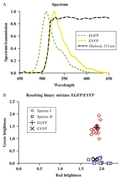
Resolving EGFP/EYFP mixtures in living cells. (A) The emission spectra of EGFP (green dotted line) and EYFP (solid line) are plotted together with the transmission curve (dashed line) of the dichroic mirror used to separate the fluorescence into two channels. (B) EGFP and EYFP are transiently expressed in COS cells. Cells were measured for 5 min in the nucleus. The data were fitted to a two-species dual-color TIFCA model. The brightness of each species (λR,λG) is represented as a point in the brightness signature plot. The brightness of species I is close to that of the EGFP (+), and the brightness of species II is close to that of EYFP (X). The EGFP and EYFP brightness signature are obtained in advance by a calibration experiment.
3.5. Measure protein interaction with heterospecies partition analysis
In the previous section, we showed that it is possible to obtain nine statistically significant bivariate cumulants in live-cell experiments and a binary protein mixture can be reliably resolved with a single measurement. Thus, dual-color brightness analysis has tremendous potential for studying protein heterointeractions. However, heterointeractions between two proteins, D and A, result generally in a mixture of at least three species (D, A, DA, DA2, etc.). Unfortunately, a general analysis method for extracting the brightness of three or more species from a heterogeneous sample is not available. Recently, we introduced heterospecies partition analysis to tackle a general interaction scheme between two proteins D+nA↔DAn. We label protein D with EGFP and A with mCherry. With proper choice of filters, it is possible to eliminate the green channel fluorescence of mCherry completely (Fig. 5.6A). HSP combines all hetero interacting molecules into a single heterospecies H={D, DA, DA2, …} (Fig. 5.6B). Using the two first-order and three second-order cumulants, and with the proper choice of filter set, the red channel brightness of heterospecies λH is analytically related to the stoichiometry n and the degree of binding (Wu, Chen, & MüCller, 2010).
Figure 5.6.

(A) The spectra of EGFP (green dash) and mCherry (purple solid) are plotted together with the transmission curve of the dichroic mirror (black dash-dot) and the emission filter in the green channel (blue dot). This filter set completely eliminates fluorescence contributions of mCherry to the green detection channel. (B) Conceptual picture illustrating the projection of a mixture of brightness species into two different classes. One class contains the molecules of A that are not interacting with D, which is referred to as free species (A, A2, …, Ar). The other class includes all species that contain the molecule D (D, DA, DA2, …, DAs) and is called heterospecies. The FFS parameters describing the heterospecies characterize the binding between D and A. (C) Full-length EGFP-TIF2 and mCherry-RXR are cotransfected in CV-1 cells. The cells were measured in the nuclei for 1 min. The bivariate factorial cumulants are fitted by dual-color TIFCA to a two-species HSP model. As a result, the brightness of the heterospecies is recovered. The red channel brightness of the heterospecies is plotted as a function of mCherry-RXR concentration. The theoretical brightness of a hetero-dimer and that of a hetero-trimer are shown as solid lines for reference. In the absence of ligand (triangle), there is only weak interaction. In the presence of ligand 9-cis retinoic acid (diamond), EGFP-TIF2 interacts strongly with mCherry-RXR and binds to as many as two mCherry-RXR molecules at high concentrations.
We apply HSP to study the interaction between RXR and a coactivator transcription intermediate factor-2 (TIF2) (Wu et al., 2010). Cells expressing mCherry-RXR and EGFP-TIF2 are measured in the nucleus of CV-1 cells. The brightness of the heterospecies is determined by dualcolor TIFCA fit to the two-species HSP model. The red channel brightness of the heterospecies is shown in Fig. 5.6C as a function of mCherry-RXR concentration. Without ligand the interaction between RXR and coactivator is weak with less than one NR bound per coactivator molecule on average. The strength of interaction increases if the ligand is present. At the lowest concentration, the brightness of the heterospecies is close to that of EGFP, indicating that EGFP-TIF2 and mCherry-RXR do not interact with each other. The brightness increases with growing RXR concentration and saturates at a brightness, which corresponds to the hetero-trimer TIF2–RXR2. Thus, the experiment demonstrates that RXR and TIF2 interact in the presence of ligand and two nuclear receptors are recruited by one coactivator. Previous in vitro and in vivo experiments based on fragments of nuclear receptor and coactivator shows distinct binding stoichiometry (Chen & Müller, 2007; Margeat et al., 2001; Teichert et al., 2009). With full-length proteins, a 2:1 stoichiometry between NRs to coactivator was observed, which confirms the bindingmodel suggested frominteraction between NR and its hormone response elements (Xu, Glass, & Rosenfeld, 1999).
4. Conclusion
In this chapter, we reviewed the technique of TIFCA for the analysis of FFS experiment. TIFCA differs from other methods by using the factorial cumulants of photon counts to extract information. In contrast to PCH, FIDA or FIMDA, TIFCA is exact for all sampling times. A central concept of the theory is the binning function, which characterizes the influence of sampling time on cumulants. The error analysis of cumulants allows experimentalist to measure or predict whether experimental conditions are sufficient for resolving species and helps in identifying optimal experimental conditions. Nonideal photodetector effects on cumulants are also taken into account in the theory. In practice, parameters are reliably recovered for a concentration range of three orders of magnitude. Statistical significant higher order cumulants established by TIFCA help in resolving binary mixtures and in determining the oligomerization of proteins that is difficult to achieve with other analysis methods. By combining heterospecies partition analysis with dual-color TIFCA, we are able to determine the oligomerization and binding curve of a general type of protein heterointeractions. This paper demonstrates the significant potential of TIFCA as a sensitive and robust technique to characterize molecular interaction in living cells.
Acknowledgments
We thank Jinhui Li for providing data about EGFP-RXR in the absence of ligand. B. W. is supported by grants from NIH GM84364 and GM86217 to R. H. S. J. D. M. is supported by grants from NIH GM64589 and NSF 0346782.
References
- Berland KM, So PT, Gratton E. Two-photon fluorescence correlation spectroscopy: Method and application to the intracellular environment. Biophysical Journal. 1995;68(2):694–701. doi: 10.1016/S0006-3495(95)80230-4. [DOI] [PMC free article] [PubMed] [Google Scholar]
- Bertrand E, Chartrand P, Schaefer M, Shenoy SM, Singer RH, Long RM. Localization of ASH1 mRNA particles in living yeast. Molecular Cell. 1998;2(4):437–445. doi: 10.1016/s1097-2765(00)80143-4. [DOI] [PubMed] [Google Scholar]
- Chao JA, Patskovsky Y, Almo SC, Singer RH. Structural basis for the coevolution of a viral RNA-protein complex. Nature Structural and Molecular Biology. 2008;15(1):103–105. doi: 10.1038/nsmb1327. [DOI] [PMC free article] [PubMed] [Google Scholar]
- Chen Y, Müller JD. Determining the stoichiometry of protein terocomplexes in living cells with fluorescence fluctuation spectroscopy. Proceedings of the National Academy of Sciences of the United States of America. 2007;104(9):3147–3152. doi: 10.1073/pnas.0606557104. [DOI] [PMC free article] [PubMed] [Google Scholar]
- Chen Y, Müller JD, So PT, Gratton E. The photon counting histogram in fluorescence fluctuation spectroscopy. Biophysical Journal. 1999;77(1):553–567. doi: 10.1016/S0006-3495(99)76912-2. [DOI] [PMC free article] [PubMed] [Google Scholar]
- Chen Y, Wei LN, Müller JD. Probing protein oligomerization in living cells with fluorescence fluctuation spectroscopy. Proceedings of the National Academy of Sciences of the United States of America. 2003;100(26):15492–15497. doi: 10.1073/pnas.2533045100. [DOI] [PMC free article] [PubMed] [Google Scholar]
- Digman MA, Gratton E. Lessons in fluctuation correlation spectroscopy. Annual Review of Physical Chemistry. 2011;62:645–668. doi: 10.1146/annurev-physchem-032210-103424. [DOI] [PMC free article] [PubMed] [Google Scholar]
- Golding I, Paulsson J, Zawilski SM, Cox EC. Real-time kinetics of gene activity in individual bacteria. Cell. 2005;123(6):1025–1036. doi: 10.1016/j.cell.2005.09.031. [DOI] [PubMed] [Google Scholar]
- Hillesheim LN, Chen Y, Müller JD. Dual-color photon counting histogram analysis of mRFP1 and EGFP in living cells. Biophysical Journal. 2006;91(11):4273–4284. doi: 10.1529/biophysj.106.085845. [DOI] [PMC free article] [PubMed] [Google Scholar]
- Hillesheim LN, Müller JD. The photon counting histogram in fluorescence fluctuation spectroscopy with non-ideal photodetectors. Biophysical Journal. 2003;85(3):1948–1958. doi: 10.1016/S0006-3495(03)74622-0. [DOI] [PMC free article] [PubMed] [Google Scholar]
- Huang B, Perroud TD, Zare RN. Photon counting histogram: One-photon excitation. ChemPhysChem. 2004;5(10):1523–1531. doi: 10.1002/cphc.200400176. [DOI] [PubMed] [Google Scholar]
- Kask P, Palo K, Ullmann D, Gall K. Fluorescence-intensity distribution analysis and its application in biomolecular detection technology. Proceedings of the National Academy of Sciences of the United States of America. 1999;96(24):13756–13761. doi: 10.1073/pnas.96.24.13756. [DOI] [PMC free article] [PubMed] [Google Scholar]
- Kendall MG, Stuart A. Chapter 3: Moments and cumulants. The advanced theory of statistics. New York: MacMillan Publishing Co., Inc.; 1977a. pp. 57–96. [Google Scholar]
- Kendall MG, Stuart A. Chapter 12: Cumulants of sampling distributions (1). The advanced theory of statistics. New York: MacMillan Publishing Co., Inc.; 1977b. pp. 293–328. [Google Scholar]
- Larson DR, Zenklusen D, Wu B, Chao JA, Singer RH. Real-time observation of transcription initiation and elongation on an endogenous yeast gene. Science. 2011;332(6028):475–478. doi: 10.1126/science.1202142. [DOI] [PMC free article] [PubMed] [Google Scholar]
- Magde D, Elson E, Webb WW. Thermodynamics fluctuations in a reacting system: Measurement by fluorescence correlation spectroscopy. Physical Review Letters. 1972;29:705–708. [Google Scholar]
- Margeat E, Poujol N, Boulahtouf A, Chen Y, Müller JD, Gratton E, et al. The human estrogen receptor alpha dimer binds a single SRC-1 coactivator molecule with an affinity dictated by agonist structure. Journal of Molecular Biology. 2001;306(3):433–442. doi: 10.1006/jmbi.2000.4418. [DOI] [PubMed] [Google Scholar]
- Müller JD. Cumulant analysis in fluorescence fluctuation spectroscopy. Biophysical Journal. 2004;86(6):3981–3992. doi: 10.1529/biophysj.103.037887. [DOI] [PMC free article] [PubMed] [Google Scholar]
- Müller JD, Chen Y, Gratton E. Resolving heterogeneity on the single molecular level with the photon-counting histogram. Biophysical Journal. 2000;78(1):474–486. doi: 10.1016/S0006-3495(00)76610-0. [DOI] [PMC free article] [PubMed] [Google Scholar]
- Palmer AG, Thompson NL. High-order fluorescence fluctuation analysis of model protein clusters. Proceedings of the National Academy of Sciences of the United States of America. 1989;86(16):6148–6152. doi: 10.1073/pnas.86.16.6148. [DOI] [PMC free article] [PubMed] [Google Scholar]
- Palo K, Mets U, Jäger S, Kask P, Gall K. Fluorescence intensity multiple distributions analysis: Concurrent determination of diffusion times and molecular brightness. Biophysical Journal. 2000;79(6):2858–2866. doi: 10.1016/S0006-3495(00)76523-4. [DOI] [PMC free article] [PubMed] [Google Scholar]
- Perroud TD, Huang B, Zare RN. Effect of bin time on the photon counting histogram for one-photon excitation. ChemPhysChem. 2005;6(5):905–912. doi: 10.1002/cphc.200400547. [DOI] [PubMed] [Google Scholar]
- Rigler R, Mets U, Widengren J, Kask P. Fluorescence correlation spectroscopy with high count rate and low background: Analysis of translational diffusion. European Biophysical Journal. 1993;22:169–175. [Google Scholar]
- Saffarian S, Elson EL. Statistical analysis of fluorescence correlation spectroscopy: The standard deviation and bias. Biophysical Journal. 2003;84(3):2030–2042. doi: 10.1016/S0006-3495(03)75011-5. [DOI] [PMC free article] [PubMed] [Google Scholar]
- Saleh B. Photoelectron statistics. New York: Springer-Verlag; 1978. [Google Scholar]
- Schwille P, Kummer S, Heikal AA, Moerner WE, Webb WW. Fluorescence correlation spectroscopy reveals fast optical excitation-driven intramolecular dynamics of yellow fluorescent proteins. Proceedings of the National Academy of Sciences of the United States of America. 2000;97(1):151–156. doi: 10.1073/pnas.97.1.151. [DOI] [PMC free article] [PubMed] [Google Scholar]
- Slaughter BD, Li R. Toward quantitative “in vivo biochemistry” with fluorescence fluctuation spectroscopy. Molecular Biology of the Cell. 2010;21(24):4306–4311. doi: 10.1091/mbc.E10-05-0451. [DOI] [PMC free article] [PubMed] [Google Scholar]
- Teichert A, Arnold LA, Otieno S, Oda Y, Augustinaite I, Geistlinger TR, et al. Quantification of the vitamin D receptor-coregulator interaction. Biochemistry. 2009;48(7):1454–1461. doi: 10.1021/bi801874n. [DOI] [PMC free article] [PubMed] [Google Scholar]
- Tetin SY, Ruan Q, Saldana SC, Pope MR, Chen Y, Wu H, et al. Interactions of two monoclonal antibodies with BNP: High resolution epitope mapping using fluorescence correlation spectroscopy. Biochemistry. 2006;45(47):14155–14165. doi: 10.1021/bi0607047. [DOI] [PubMed] [Google Scholar]
- Webb WW. Fluorescence correlation spectroscopy: Inception, biophysical experimentations, and prospectus. Applied Optics. 2001;40:3969–3983. doi: 10.1364/ao.40.003969. [DOI] [PubMed] [Google Scholar]
- Wu B, Chao JA, Singer RH. Fluorescence fluctuation spectroscopy enables quantitative imaging of single mRNAs in living cells. Biophysical Journal. 2012;102(12):2936–2944. doi: 10.1016/j.bpj.2012.05.017. Epub 2012, June 19. [DOI] [PMC free article] [PubMed] [Google Scholar]
- Wu B, Chen Y, Müller JD. Dual-color time-integrated fluorescence cumulant analysis. Biophysical Journal. 2006;91(7):2687–2698. doi: 10.1529/biophysj.106.086181. [DOI] [PMC free article] [PubMed] [Google Scholar]
- Wu B, Chen Y, Müller JD. Heterospecies partition analysis reveals binding curve and stoichiometry of protein interactions in living cells. Proceedings of the National Academy of Sciences. 2010;107(9):4117–4122. doi: 10.1073/pnas.0905670107. [DOI] [PMC free article] [PubMed] [Google Scholar]
- Wu B, Müller JD. Time-integrated fluorescence cumulant analysis in fluorescence fluctuation spectroscopy. Biophysical Journal. 2005;89:2721–2735. doi: 10.1529/biophysj.105.063685. [DOI] [PMC free article] [PubMed] [Google Scholar]
- Xu L, Glass CK, Rosenfeld MG. Coactivator and corepressor complexes in nuclear receptor function. Current Opinion in Genetics and Development. 1999;9(2):140–147. doi: 10.1016/S0959-437X(99)80021-5. [DOI] [PubMed] [Google Scholar]
- Zimyanin VL, Belaya K, Pecreaux J, Gilchrist MJ, Clark A, Davis I, et al. In vivo imaging of oskar mRNA transport reveals the mechanism of posterior localization. Cell. 2008;134(5):843–853. doi: 10.1016/j.cell.2008.06.053. [DOI] [PMC free article] [PubMed] [Google Scholar]