Abstract
Low-dose computed tomography (CT) imaging without sacrifice of clinical tasks is desirable due to the growing concerns about excessive radiation exposure to the patients. One common strategy to achieve low-dose CT imaging is to lower the milliampere-second (mAs) setting in data scanning protocol. However, the reconstructed CT images by the conventional filtered back-projection (FBP) method from the low-mAs acquisitions may be severely degraded due to the excessive noise. Statistical image reconstruction (SIR) methods have shown potentials to significantly improve the reconstructed image quality from the low-mAs acquisitions, wherein the regularization plays a critical role and an established family of regularizations is based on the Markov random field (MRF) model. Inspired by the success of nonlocal means (NLM) in image processing applications, in this work, we propose to explore the NLM-based regularization for SIR to reconstruct low-dose CT images from low-mAs acquisitions. Experimental results with both digital and physical phantoms consistently demonstrated that SIR with the NLM-based regularization can achieve more gains than SIR with the well-known Gaussian MRF regularization or the generalized Gaussian MRF regularization and the conventional FBP method, in terms of image noise reduction and resolution preservation.
Keywords: low-dose CT, statistical image reconstruction, nonlocal means, regularization
1. Introduction
X-ray computed tomography (CT) has been widely exploited in clinic. Recent discoveries regarding the potential harmful effects of X-ray radiation including genetic and cancerous diseases have raised growing concerns to patients and medical physics community [1]. Low-dose CT is highly desirable while maintaining satisfactory image quality for a specific clinical task. One common strategy to achieve low-dose CT imaging is to lower the milliampere-second (mAs) setting (by lowering X-ray tube current and/or shortening the exposure time) in CT scanning protocol. However, without adequate treatments in image reconstruction, the images from the low-mAs acquisitions will be severely degraded due to the excessive noise.
Many methods have been proposed to improve the image quality with low-dose CT [2–15]. Among them, statistical image reconstruction (SIR) methods, which take into account of statistical properties of the projection data and accommodate the imaging geometry, have shown to be superior in suppressing noise and streak artifacts as compared to the conventional filtered back-projection (FBP) method. According to the maximum a posterior (MAP) estimation criteria, the SIR methods can be typically formulated with an objective function consisting of two terms: the data-fidelity term modeling the statistics of measured data, and the regularization term reflecting a prior information about the image map. Minimizing the objective function is routinely performed by an iterative algorithm.
Previous studies have revealed two principal sources of the CT transmission data noise: (1) X-ray quanta noise due to limited number of detected photons, and (2) system electronic noise due to electronic fluctuation [16–20]. The X-ray quanta can be described by the compound Poisson model [21–23] by considering the polychromatic X-ray generation. However, it lacks an analytical probability density function (PDF) expression which impedes its use in SIR methods. Instead, a simple Poisson model is well accepted and has been widely used in SIR methods [4–6, 9–13]. The electronic fluctuation generally follows a Gaussian distribution, and the mean of electronic noise is often calibrated to be zero in order to reduce the effect of detector dark current [18–20]. Consequently, a statistically independent Poisson distribution plus a zero-mean Gaussian distribution has been extensively utilized to describe the acquired CT transmission data and to develop the SIR framework for low-dose CT [24,25].
Extensive experiments have shown that the regularization term in the objective function of SIR plays a critical role for successful image reconstruction [10–15]. One established family of regularizations is based on the Markov random field (MRF) model [26,27] which describes the statistical distribution of a voxel (or pixel in two-dimensional (2D) space) given its neighbors. Those regularizations generally rely on pixel values within a local fixed neighborhood and give equal weighting coefficients for the neighbors of equal distance without considering structure information in images. A quadratic-form regularization, which corresponds to the Gaussian MRF prior, has been widely used for iterative image reconstruction [4,9,12,13]. Other regularizations of this family adjust the potential function to penalize large differences between neighboring pixels less than the quadratic function while maintaining the similar level of penalty for small differences so as to better preserve edges [27–33]. However, the reconstruction results could be sensitive to the choice of “transition point” (or edge threshold) which controls the shape of the potential function [32]. Overall, this family of regularizations is inherently local and lack global connectivity or continuity.
The nonlocal means (NLM) algorithm was introduced by Buades et al for image de-noising [34,35]. Essentially, it is one of the nonlinear neighborhood filters which reduce image noise by replacing each pixel intensity with a weighted average of its neighbors according to the similarity. The similarity comparison could be performed between any two pixels within the entire image, although it is limited to a fixed neighboring window area (e.g., 17×17) of target pixel for computation efficiency in practice. Inspired by its success in image processing scenario, researchers further extended it to the medical imaging applications such as the low-dose CT. For instance, Giraldo et al [36] examined its efficacy on CT images for noise reduction. Ma et al [37] tried to restore the low-mAs CT images using previous normal-dose scan via the NLM algorithm, and observed noticeable gains over the traditional NLM filtering. Similarly, Xu and Muller [38] added effort to restore the sparse view CT images using high quality prior scan and artifact-matched prior scan with the NLM algorithm and also noticed remarkable improvements. However, these methods [36–38] are essentially post-reconstruction filtering or restoration, which do not fully take advantage of the projection data. The traditional NLM filtering [36] sometimes cannot completely eliminate the noise and streak artifacts. The extensions [37,38] need high quality prior scan and necessary registration to align the images from two different scans. Furthermore, researchers also explored the NLM-based regularizations for several inverse problems [39–50], including image reconstructions for magnetic resonance imaging [45], positron emission tomography [41,47] and X-ray CT [43,46,48,50]. For instance, Tian et al [46] presented a temporal NLM regularization for 4D dynamic CT reconstruction, where the reconstruction of current frame image utilizing two neighboring frame images. Ma et al [48, 50] proposed previous normal-dose CT scan induced NLM regularizations to improve the follow-up low-dose CT scans reconstruction. However, for some applications, the neighboring frame images or previous normal-dose scan may not be available. In this study, we explored to incorporate a NLM-based generic regularization into the SIR framework for low-dose CT, wherein the regularization only utilizes information of the current scan.
The remainder of this paper is presented as follows. Section II derives the SIR framework for low-dose CT in the presence of electronic noise, followed by the regularization term based on the NLM algorithm. Section III evaluates the NLM-based regularization using both digital and physical phantom datasets. After a discussion of existing issues and future research topics, we draw conclusions of this study in Section IV.
2. Methods
2.1. Statistical image reconstruction (SIR) framework for low-dose CT
Under the assumption of monochromatic X-ray generation, the CT measurement can be approximately expressed as a discrete linear system:
| (1) |
where ȳ = (ȳ1, ȳ2, …, ȳI)T denotes the vector of expected line integrals, and I is the number of detector bins; μ = (μ1, …, μJ)T represents the vector of attenuation coefficients of the object to be reconstructed, and J is the number of image pixels; A is the system or projection matrix with the size I×J and its element Aij is typically calculated as the intersection length of projection ray i with pixel j.
The line integral along an attenuation path is calculated according to the Lambert-Beer’s law:
| (2) |
where N0i represents the mean number of X-ray photons just before entering the patient and going toward the detector bin i, and can be measured by system calibration, e.g., by air scans; Ni denotes the detected photon counts at detector bin i with expected value N̄i. The approximation for the second equation in (2) reflects an assumption that the Lambert-Beer’s law can be applied to the random values.
Previous investigations [18–20] have revealed two principal sources of CT transmission data noise, X-ray quanta noise and system electronic noise. With the assumption of monochromatic X-ray generation, the acquired CT transmission data (detected photon counts) can be described as:
| (3) |
where is the variance of electronic noise.
Based on the noise model (3) and the use of the Lambert-Beer’s law (2), the relationship between the mean and variance of the line integral measurements (or log-transformed data) can be described by the following formula [20,51,52]:
| (4) |
Previous studies showed that the noisy line integral measurements can be treated as normally distributed with a nonlinear signal-dependent variance [53, 54]. Assuming the measurements among different bins are statistically independent, the likelihood function of the joint probability distribution, given a distribution of the attenuation coefficients, can be written as:
| (5) |
where y = (y1, …, yI)T is the vector of measured line integrals, and Z is a normalizing constant.
Omitting the constant terms, the corresponding log-likelihood function can be written as:
| (6) |
Mathematically, low-dose CT reconstruction represents an ill-posed problem due to the presence of noise in projection data. Therefore, the image estimate that maximizes L(y | μ) is very noisy and unstable. The Bayesian methods could improve the quality of reconstructed images by introducing a prior (or equivalently, a regularization term) to regularize the solution. Consequently, the low-dose CT reconstruction is usually formulated as:
| (7) |
where U (μ) denotes the regularization term and β is the smoothing parameter that controls the tradeoff between the data fidelity and regularization term.
2.2. Markov random field (MRF) model based regularizations
Under the MRF model, a family of regularization terms is widely used for iterative image reconstruction [4–13, 27–33]:
| (8) |
where index j runs over all the pixels in the image domain, Fj denotes the small fixed neighborhood (typically 8 neighbors in the 2D case) of the jth image pixel, and wjm is the weighting coefficient that indicates the interaction degree between central pixel j and its neighboring pixel m. Usually the weighting coefficient is determined by the inverse of the Euclidean distance between the two pixels. Thus, in 2D case, wjm = 1 for the four horizontal and vertical neighboring pixels, for the four diagonal neighboring pixels, and wim = 0 otherwise. The ϕ denotes a positive potential function, and when ϕ(Δ) = Δ2/2, Eq. (8) corresponds to the Gaussian MRF (GMRF) regularization which has been widely used for iterative image reconstruction [4,9,12,13]. The major drawback of the GMRF regularization is that it fails to take the discontinuities in images into account, thus it may lead to over smoothing of edges or fine structures in the reconstructed images. To address this issue, researchers [27–33] replaced the quadratic potential function with non-quadratic functions such as ϕ(Δ) = |Δ|p (1< p< 2) , which induces the edge-preserving generalized Gaussian MRF (GGMRF) regularization [32]. In this study, p was set to 1.5 for all the cases to illustrate the performance of the GGMRF regularization.
2.3. Nonlocal means (NLM) algorithm based regularizations
2.3.1. Overview of the NLM algorithm
The NLM algorithm was proposed by Buades et al [34,35] for removing noise while preserving edge information in an image. It is one of the nonlinear neighborhood filters and reduces image noise by replacing each pixel intensity with a weighted average of its neighbors according to their similarity. While previous neighborhood filters calculate the similarity based on intensity value in a single pixel, the NLM is based on patch and is believed to be more robust since the intensity value in a single pixel is noisy. A patch of a pixel is defined as a squared region centered at that pixel (e.g., 5×5, called patch-window (PW) ). Let P(μ̂j) denote the patch centered at pixel j and P(μ̂k) denote the patch centered at pixel k. The similarity between pixels j and k depends on the weighted Euclidean distance of their patches, , which is computed as the distance of two intensity vectors in high dimensional space with a Gaussian kernel (a>0 is the standard deviation of the Gaussian kernel) to weight the contribution for each dimension. The exponential function converts the similarity to weighting coefficient which indicates the interaction degree between two pixels. The weighting coefficient is positive and symmetric, i.e., wjk>0 and wjk=wkj. The filtering parameter h controls the decay of the exponential function and accordingly the decay of weighting coefficient as the function of two patches’ distance. Also, the similarity comparison is limited to a fixed neighboring window area (e.g., 17×17, called search-window (SW)) of the target pixel for computation efficiency in practice.
Mathematically, the NLM algorithm can be describes as [34,35]:
| (9) |
where , the vector μ̂ = (μ̂1, …,μ̂J)T represents the noisy image to be smoothed, Sj denotes the SW of pixel j in two dimensions, k denotes the pixel within the SW of pixel j and its weighting coefficient wjk is normalized to force the sum of neighboring pixel weight to be 1, and μ̌j,NLM is the intensity value of pixel j after the NLM filtering.
2.3.2. NLM based regularizations
Motivated by the work of NLM filter, Buades et al. [39] proposed the regularization model:
| (10) |
where μ̃ is a reference image, and the weighting coefficient wjk (μ̃) is calculated from μ̃. However, a good reference image is usually not available before image reconstruction for low-dose CT. Lou et al. [43] suggested to use the FBP reconstruction result as the reference image, but such a reference image is typically noisy and the resulted regularization in Eq. (10) may lead to suboptimal reconstruction result.
To improve the reconstruction accuracy, in this work, we intend to make the regularization model be generic and thus take the following form:
| (11) |
where . There are several choices for the potential function, but in this study, we only explored the regularization where ϕ(Δ) = Δ2/2. This choice makes the cost function in (7) be quadratic and easy to optimize. We also utilized this as an example to demonstrate the feasibility and efficacy of the presented NLM-based regularizations for low-dose CT reconstruction, although some other potential functions (e.g. ϕ(Δ) = |Δ|p (1< p< 2) may further improve the performance.
2.4. Optimization approach and implementation issue
In Eq. (11), since the weighting coefficients in the regularization are computed on the unknown image μ, direct minimization of the objective function in (7) using the regularization in (11) can be very complicated. Instead, an empirical one-step-late (OSL) implementation is employed, based on the Gauss-Seidel (GS) updating strategy [55], for the minimization task in this study, where the weighting coefficients are computed on current image estimate and then are assumed to be constants when updating the image [41,44,45]. In addition, the sinogram variance is also undated in each iteration according to Eq. (4) for more accurate estimation. Although there is no proof of global convergence for such an OSL iteration scheme, it is observed that the image estimation converges to a steady status after 20 iterations (the difference between the estimated images of two successive iterations becomes very small) for all the datasets presented in this study.
The pseudo-code for the statistical CT image reconstruction with the presented NLM-based regularization is listed as follows (where Aj denotes the jth column of the projection matrix A):
Initialization:
μ̂ = FBP{y};q = Aμ̂; r̂ = y−q; D = diag{1/σ2(yi)};
For each iteration:
begin
updating wjk based on current image estimation
For each pixel j:
begin
end
end
3. Experiments and Results
In this study, computer simulated digital phantom and experimental physical phantoms were utilized to evaluate the performance of statistical image reconstruction using the presented NLM-based regularization (referred to as SIR-NLM), with comparison to that using the GMRF regularization (referred to as SIR-GMRF) or GGMRF regularization (p=1.5, referred to as SIR-GGMRF) and the classical FBP reconstruction.
3.1. Digital NCAT phantom
3.1.1. Data simulation
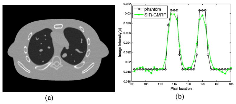
The NCAT phantom was used in this study as it provides a realistic model of human anatomy [56]. Each slice of the phantom is composed of 512×512 pixels with pixel size 1.0×1.0 mm. We chose a geometry that was similar to the fan-beam Siemens SOMATOM Sensation 16 CT scanner setup: i) the distance from the rotation center to the X-ray source is 570 mm and the distance from the arc detector array to the X-ray source is 1040 mm; ii) Each rotation includes 1160 projection views evenly spanned on a 360° circular orbit; iii) Each view has 672 detector bins and the space of each detector bin is 1.407 mm. Similar to the study of La Rivière et al [24,25], after calculating the noise-free line integrals ȳ based on model (1), the noisy measurement Ni at detector bin i was generated according to the statistical model:
| (12) |
where N0i is set to 2×10⁴ and is set to 10 [24] for low-dose scan simulation in this study. Then the corresponding noisy line integral yi is calculated by the logarithm transform.
3.1.2. Parameter selection
I) NLM filter related parameters
Determining the optimal parameters for NLM filter is not a trivial task [37]. Since the primary goal of this research is to demonstrate the feasibility and effectiveness of the presented NLM-based regularization, the parameters were empirically set through extensive experiments by visual inspection and quantitative measures in this study. We found a 17×17 search-window (or SW) and 5×5 patch-window (or PW) (the standard deviation a of the Gaussian kernel is set to be 5) could achieve a good compromise between noise suppression and computational efficiency. Therefore, this set of parameters was used for all of our following implementations. The filtering parameter h is a function of the standard deviation of the image noise according to [35], however, the noise distribution of low-dose CT image is non-stationary and unknown. Therefore, it is also empirically set via the extensive trial-and-error process in this study. Larger value of h will result in more smoothing while too small value of h could induce artifacts.
II) Smoothing parameter β of SIR methods
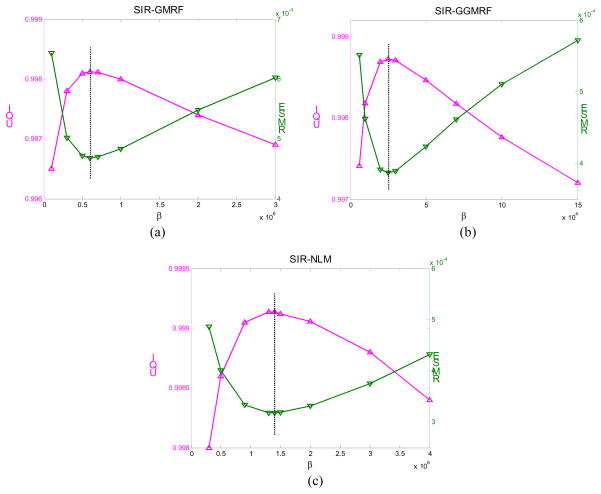
After the NLM related parameters are chosen, we further determine the smoothing parameter β. The parameter β controls the tradeoff between the data fidelity term and the regularization term of the SIR objective function. In this study, a series of β values were tested for the three SIR methods. After the images were reconstructed, two quantitative metrics were used to determining the optimal β value for each method. The first metric is the traditional root mean squared error (RMSE), which indicates the difference between the reconstructed image and the ground truth image and characterizes the reconstruction accuracy. The second metric is the universal quality index (UQI) [57] which measures the similarity between the reconstructed image and the ground truth image. The UQI quantifies the noise, spatial resolution, and texture correlation between two images, and has been widely used in CT image quality evaluation during the past few years [58–60].
Let μr denote the vector of the reconstructed image and μ0 be the vector of the ground truth image(digital phantom), the two metrics are defined as:
| (13) |
| (14) |
where
The β value that offered the lowest RMSE and highest UQI is considered as the optimal β and was used in the following evaluations. This procedure of choosing optimal β value presented here is a little similar to that in [12], but much easier to implement. Also, it is applied after a series of images reconstructed rather than before the image reconstruction.
3.1.3. Visualization-based evaluation
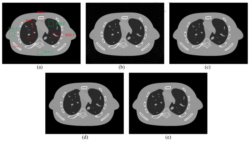
The reconstructed images by the FBP, SIR-GMRF, SIR-GGMRF and SIR-NLM from simulated noisy sinogram are shown in figure 2. It can be observed that all the three SIR methods outperformed the FBP in terms of noise and streak artifact suppression, which is attributed to the explicit statistical modeling of sinogram data. As for the three SIR methods, the SIR-NLM is superior in noise reduction and edge preservation, which will be quantified in the following section.
Figure 2.
One transverse slice of the NCAT phantom: (a) phantom; (b) reconstruction result with FBP from simulated noisy sinogram; (c) reconstruction result with SIR-GMRF from simulated noisy sinogram (β=6×10⁵); (d) reconstruction result with SIR-GGMRF from simulated noisy sinogram (β=2.5×10⁴); (e) reconstruction result with the proposed SIR-NLM from simulated noisy sinogram (β=1.4×10⁶, SW=17×17, PW=5×5, h=0.007). All the images are displayed with the same window.
3.1.4. Quantitative evaluation
With the optimal β values from figure 1, the overall RMSE (or UQI) for the reconstructed images are 4.68×10⁻⁴ (0.9981), 3.87×10⁻⁴ (0.9987) and 3.18×10⁻⁴ (0.9991) by the SIR-GMRF, SIR-GGMRF, and SIR-NLM, respectively. Meanwhile, the overall RMSE (or UQI) for the reconstructed image by the FBP method is 1.24×10⁻³ (0.9870). These results quantitatively reveal that the SIR-NLM generated the best overall image quality, which is consistent with the visual inspection.
Figure 1.
Illustration of determining the optimal β value for three SIR methods.
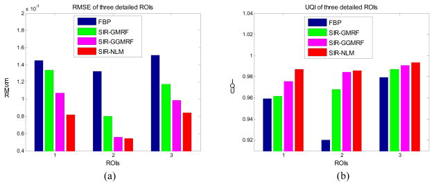
Furthermore, we compare the performance of the four methods on the reconstruction of small regions of interest (ROIs) with detailed structures as indicated by the red rectangles in figure 2(a). The corresponding quantitative results with RMSE and UQI are shown in figure 3. Still, the SIR-NLM offered the best image quality for the three detailed ROIs.
Figure 3.
Performance comparison of the four methods on the reconstruction of detailed ROIs labeled in figure 2(a) with RMSE and UQI metrics. The corresponding methods are illustrated in figure legend.
3.1.5. Noise and resolution tradeoff
Herein, we further evaluate the reconstruction results by the four methods with quantitative metrics in terms of noise reduction and resolution preservation.
I) Noise reduction
In this study, the noise reduction of the reconstructed images was quantified by the standard deviation (STD) and mean percent absolute error (MPAE) of two uniform regions with 30×30 pixels, as shown in the green boxes of figure 2(a). The two metrics are defined as:
| (15) |
| (16) |
Table 1 demonstrated that the proposed SIR-NLM has the best performance in noise reduction with the smallest STD and MPAE.
Table 1.
Noise reduction of two uniform regions in figure 2(a) by the four reconstruction methods
| Methods | ROI A | ROI B | ROI C | |||
|---|---|---|---|---|---|---|
| STD (×10−4) | MPAE | STD (×10−4) | MPAE | STD (×10−4) | MPAE | |
| FBP | 16.63 | 7.29 | 12.55 | 18.77 | 15.45 | 6.68 |
| SIR-GMRF | 5.95 | 2.55 | 6.16 | 9.33 | 6.07 | 2.64 |
| SIR-GGMRF | 3.86 | 1.63 | 3.90 | 5.61 | 3.78 | 1.60 |
| SIR-NLM | 3.66 | 1.57 | 3.78 | 5.71 | 3.48 | 1.51 |
II) Resolution preservation
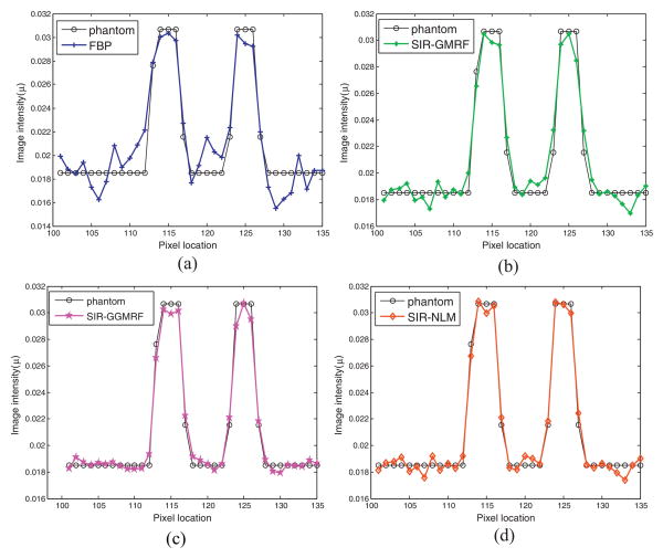
The image resolution can be characterized by the horizontal profile labeled by a red line in figure 2(a). The profiles comparison with the ground truth clearly demonstrated advantage of the proposed SIR-NLM over the other three methods on the edge preservation, as illustrated in figure 4.
Figure 4.
Comparison of the profiles along the horizontal line labeled in figure 2(a) between the four methods and the ground truth. The corresponding methods are illustrated in figure legend.
This section demonstrates that the SIR-NLM offers the best noise reduction, while at the same time, the best resolution preservation. The smoothing parameter β controls the noise and resolution tradeoff for the SIR methods, which means one can always sacrifice spatial resolution for a better noise performance by increasing the value of β, or vice versa. Therefore, if we increase the β value to 1.5×10⁶ for the SIR-GMRF, which makes it have the same noise reduction performance as that by the SIR-NLM in figure 2(e), the resulting image will be further blurred. Figure 5 shows the reconstructed image, and the corresponding profile as those in figure 4. Similarly, if we increase the β value for the SIR-GGMRF to make it have the matched noise level as that in figure 2(e), the resolution of the resulting image would also be degraded.
Figure 5.
(a) Reconstructed image by the SIR-GMRF from simulated noisy sinogram (β=1.5×10⁶), which has the matched noise level as that by the SIR-NLM in figure 2(e); (b) The corresponding profile as that in figure 4.
3.2. Physical CatPhan® 600 phantom
3.2.1. Data acquisition
A commercial calibration phantom CatPhan® 600 (The Phantom Laboratory, Inc., Salem, NY) was used to evaluate the performance of the presented method. The projection data were acquired by ExactArms of a Trilogy treatment system (Varian Medical Systems, Palo Alto, CA). The source-to-detector distance is 150cm while the source-to-axis distance is 100cm. Two scans were performed at different mA levels: 80mA (normal dose), 10mA (low dose). A total of 634 projection views were collected for a full 360 rotation with X-ray pulse duration at each projection view 10 ms. The dimension of each acquired projection data is 397mm×298mm, containing 1024×768 pixels. To save the computational time, a 2×2 binning was performed. Then, the central slice sinogram data (512 bins×634 views)was extracted for this study. The size of the reconstructed image is 350×350 with pixel size of 0.776 × 0.776 mm2.
3.2.2. Visualization-based evaluation
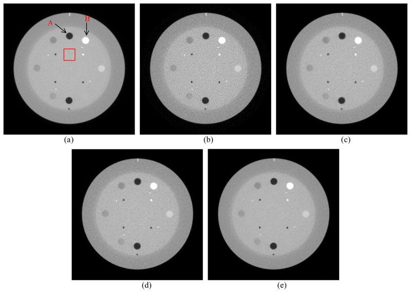
Figure 6 shows the reconstructed images of CatPhan® 600 phantom by the FBP method from the 80 mA sinogram, and by the FBP, SIR-GMRF, SIR-GGMRF and SIR-NLM from the low-dose 10mA sinogram. The corresponding β values for the three SIR methods were chosen to make their reconstructed images have matched noise level, as indicated with the dot-dash line in figure 8(a) (STD=4.5×10⁻⁴). Herein, the noise level was characterized by the standard deviation of a uniform area with 30×30 pixels, as labeled with the red square in figure 6(a). We can see that all the three SIR methods suppress noise to a large extent compared with the FBP reconstruction, and the SIR-NLM outperforms the other two SIR methods in edge preservation.
Figure 6.
A reconstructed slice of the CatPhan® 600 phantom: (a) FBP reconstruction from the 80mA sinogram. (b) FBP reconstruction from the 10mA sinogram; (c) SIR-GMRF reconstruction from the 10mA sinogram (β=2.5×10⁵); (d) SIR-GGMRF reconstruction from the 10mA sinogram (β=4.5×10³); (e) Proposed SIR-NLM reconstruction from the 10mA sinogram (β=2×10⁵, SW=17×17, PW=5×5, h=0.01). All the images are displayed with the same window.
Figure 8.
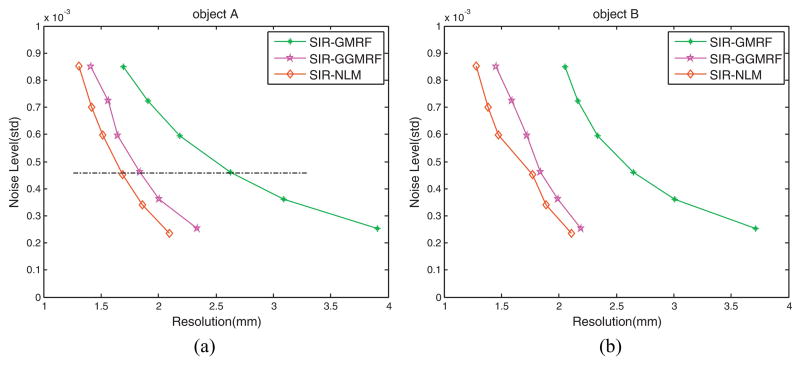
Noise-resolution tradeoff curves for the three SIR methods: (a) Comparison of the noise-resolution tradeoff curves for reconstruction of the “negative” object A labeled in figure 6(a); (b) Comparison of the noise-resolution tradeoff curves for reconstruction of the “positive” object B labeled in figure 6(a).
3.2.3. Noise-resolution tradeoff measurement
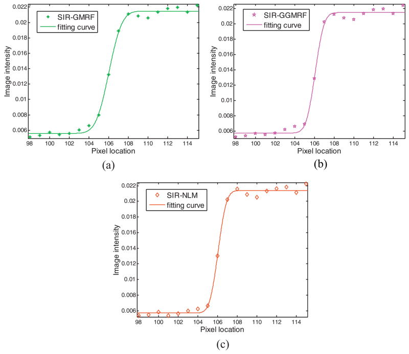
As mentioned above, the smoothing parameter β controls the tradeoff between the data fidelity term and the regularization term. A larger β value produces a more smoothed reconstruction, and vice versa. The noise-resolution tradeoff curve is an effective measure to reflect this tradeoff. In this study, the image noise was characterized by the standard deviation of a uniform area with 30×30 pixels array in background region, as labeled with the red square in figure 6(a); the image resolution was analyzed by the edge spread function (ESF) along the central vertical profiles of the “negative” object A and “positive” object B as indicated in figure 6(a). The ESF is a measure of the broadening of a step edge and the resolution is characterized by a parameter t of the fitting error function(erf) as:
| (17) |
where x is the location of the pixel and y is the corresponding pixel, y0 is the shift of the erf from zero baseline, H is the half height of the step, and x̄ is the center location of the edge.
The central vertical profiles through object A of figure 6(c)–(e) are shown in figure 7, which are also fitted with the ESF in Eq. (17). The curve fitting reveals that the image reconstructed by SIR-NLM has sharper edge than that by SIR-GMRF and SIR-GGMRF.
Figure 7.
Illustration of the ESF fitting along the central vertical profiles of object A in figure 6(c)–(e) respectively: (a) SIR-GMRF(t=1.441); (b) SIR-GGMRF(t=1.009); (c) SIR-NLM(t=0.926).
By varying the smoothing parameter β, the noise-resolution tradeoff curves for the three SIR methods with the object A and object B were obtained, as shown in figure 8. In both figures, the noise-resolution tradeoff curves of the three SIR methods show the similar trends. As the image resolution decreases, the noise level decreases. It can be observed that the SIR-NLM outperforms the SIR-GMRF and SIR-GGMRF in noise suppression at the matched resolution level (or alternatively, the SIR-NLM outperforms SIR-GMRF and SIR-GGMRF in resolution preservation at the matched noise level) for both the “negative” object A and “positive” object B. The β values that were used for plotting the tradeoff curves were summarized in Table 2.
Table 2.
A summary of β values used for the noise-resolution tradeoff measurement of the CatPhan® 600 study
| β-values | ||||||
|---|---|---|---|---|---|---|
| SIR-GMRF | 7×10⁴ | 1×10⁵ | 1.5×10⁵ | 2.5×10⁵ | 4×10⁵ | 8×10⁵ |
| SIR-GGMRF | 1.8×10³ | 2.5×10³ | 3×10³ | 4.5×10³ | 6×10³ | 1×10⁴ |
| SIR-NLM | 7×10⁴ | 1×10⁵ | 1.3×10⁵ | 2×10⁵ | 3×10⁵ | 5×10⁵ |
3.3. Physical anthropomorphic head phantom
3.3.1. Data acquisition
To evaluate the methods in a more realistic situation, an anthropomorphic head phantom was also scanned twice with X-ray tube current setting 80mA (normal dose) and 10mA (low dose) respectively. All the scanning protocols are exactly the same as that in Sec 3.2.1.
3.3.2. Visualization-based evaluation
Figure 9 shows the reconstructed images of the anthropomorphic head phantom by FBP from the 80mA sinogram, and by the FBP, SIR-GMRF, SIR-GGMRF and SIR-NLM from the low-dose 10mA sinogram. The β values for the three SIR methods were chosen to make their reconstructed images have matched noise level, which was characterized by the standard deviation of a 30×30 uniform region label in figure 9(a) (std=7.1×10⁻⁴). All the three SIR methods can effectively suppress noise compared with the FBP method, but the image reconstructed by SIR-NLM has better resolution.
Figure 9.
Reconstructed images of the anthropomorphic head phantom: (a) FBP reconstruction from the 80mA sinogram; (b) FBP reconstruction from 10mA sinogram; (c) SIR-GMRF reconstruction from 10mA sinogram (β=5×10⁵); (d) SIR-GGMRF reconstruction from 10mA sinogram (β=1.1×10⁴); (e) Proposed SIR-NLM reconstruction from 10mA sinogram (β=4×10⁵, SW=17×17, PW=5×5, h=0.012). All the images are displayed with the same window.
3.3.3. Profile-based evaluation
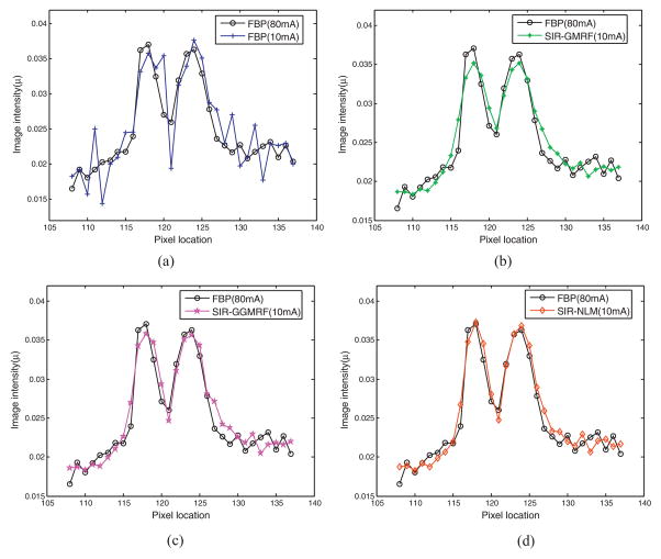
To further visualize the differences among the four reconstruction methods, horizontal profiles of the resulting images were drawn across the red line label in figure 9(a). The profiles comparison quantitatively demonstrated the advantage of the three SIR methods over the FBP method on noise suppression, as well as the merit of the proposed SIR-NLM over the SIR-GMRF and SIR-GGMRF on edge preservation at matched noise level.
4. Discussion and conclusion
A good regularization term (or equivalently, prior/penalty term) is the key to solve ill-posed inverse problems such as low-dose CT reconstruction. Effectively suppressing the noise while preserving the edges/details/ contrasts are the two major concerns when choosing a regularization. A lot of regularization terms have been studied for low-dose CT reconstruction in the past decades [4–15, 28–33]. Inspired by the success of NLM algorithm in image processing scenario, we presented, in this work, a NLM-based generic regularization for statistical image reconstruction (SIR) of low-dose CT. Experimental results with both digital and physical phantoms demonstrated that it has excellent performance in terms of image noise reduction and resolution preservation. Comparisons consistently showed the SIR with the NLM-based regularization is superior to the SIR-GMRF, SIR-GGMRF, and the classical FBP method. The performance of NLM-based regularization using other potential functions (such as ϕ(Δ) = |Δ|p (1< p< 2) remains an interesting research topic for further investigation.
Two major disadvantages of the NLM algorithm are associated with the computational burden and the related parameters tuning. Our presented regularization, which is based on the NLM algorithm, inevitably inherit these drawbacks. For the NLM-associated parameters, we empirically set the size of search-window and patch-window (also the standard deviation of the Gaussian kernel) and used that set of parameters for all our implementations. Extensive experiments showed that these parameters do not show noticeable effects on the reconstructed image when they are set in a reasonable range. The only parameter needs to be manually tuned is the filtering parameter h. The parameter h which controls the amount of de-noising is a function of the standard deviation of the image noise according to [35]. But the noise distribution of low-dose CT image is non-stationary. In this pilot study, we simply assume the image noise to be spatially invariant and set the parameter h to be a constant. However, it is noted that this assumption can be problematic and may result in imperfections in reconstructed images. Strategies to develop adaptive h considering local noise level can be a promising topic for future research to further improve the presented scheme.
The smoothing parameter β controls the tradeoff between the data fidelity term and the regularization term. A larger β value produces a more smoothed reconstruction with lower noise but also lower resolution, and vice versa. The selection of β value for the SIR methods is one of their drawbacks and is still an open question. In this study, for the digital phantom, we chose parameter β via two quantitative metrics due to the existence of ground truth, as shown in figure 1. For the two physical phantoms, we chose parameter β through visual inspection and matched noise level when we did the comparison.
One major drawback of the iterative SIR methods is their computational burden due to the multiple re-projection and back-projection operation cycles in the projection and image domains. For instance, for the reconstruction of NCAT phantom in Sec 3.1, the computation time of each iteration for SIR-GMRF, SIR-GGMRF, SIR-NLM is 168s, 173s and 201s respectively, using a PC with 3GHz CPU without any acceleration. However, with the development of fast computers and dedicated hardware [61], the computation issue may be not a problem in the near future, and the iterative SIR methods can move closer to clinical use and play an important role there.
The primary aim of this study is to investigate the feasibility and efficacy of the presented NLM-based regularization for statistical X-ray CT reconstruction. The preliminary results with both digital and physical phantoms demonstrated that it has excellent performance in terms of noise reduction and resolution preservation. Yet further evaluations using patient data are necessary to show the clinical significance and are under progress.
Figure 10.
Comparison of the profiles along the horizontal line labeled in figure 9(a) for the four methods with 10mA sinogram and the FBP reconstruction with the 80mA sinogram. The corresponding methods are illustrated in figure legend.
Acknowledgments
This work was partly supported by the National Institutes of Health under grants #CA082402 and #CA143111. JM was partially supported by the NSF of China under grant Nos. 81371544, 81000613 and 81101046 and the National Key Technologies R&D Program of China under grant No. 2011BAI12B03. JW was supported in part by grants from the Cancer Prevention and Research Institute of Texas (RP110562-P2 and RP130109) and a grant from the American Cancer Society (RSG-13-326-01-CCE). HL was supported in part by the NSF of China grants #81230035 and #81071220. The authors would also like to thank the anonymous reviewers for their constructive comments and suggestions that greatly improve the quality of the manuscript.
Appendix. SIR framework deviation for low-dose CT via the shifted Poisson approximation
It is worth noting that the criterion in Eq. (7) can also be derived via the shifted Poisson approximation. As we know, the likelihood function of model (A1) is analytically intractable:
| (A1) |
In order to circumvent this problem, however, a shifted Poisson approximation [62] can be exploited to match the first two statistical moments. With matched first and second moments, an assumption of Poisson statistics may be made. That is, the random variable approximately follows the Poisson distribution:
| (A2) |
where [x]+ = x if x>0 and is 0 otherwise.
With the shifted Poisson approximation in Eq. (A2) and omitting the constant terms, the corresponding log-likelihood function can be written as:
| (A3) |
Applying a 2nd-order Taylor expansion to around the measured line integral yi [4,5,7], we have:
| (A4) |
Ignoring the irrelevant terms, the log-likelihood in (A3) is approximated as:
| (A5) |
where . The difference between Eq. (A5) and Eqs. (4)–(6) can be ignored by the approximation of Ni ≈ N̄i.
Footnotes
Conflict of interest statement
No conflict of interest was declared by the authors.
Publisher's Disclaimer: This is a PDF file of an unedited manuscript that has been accepted for publication. As a service to our customers we are providing this early version of the manuscript. The manuscript will undergo copyediting, typesetting, and review of the resulting proof before it is published in its final citable form. Please note that during the production process errors may be discovered which could affect the content, and all legal disclaimers that apply to the journal pertain.
References
- 1.Brenner D, Hall E. Computed tomography-an increasing source of radiation exposure. The N Engl J Med. 2007;357:2277–2284. doi: 10.1056/NEJMra072149. [DOI] [PubMed] [Google Scholar]
- 2.Wang J, Lu H, Liang Z, Xing L. Recent development of low-dose cone-beam computed tomography. Current Medical Imaging Reviews. 2010;6:72–81. [Google Scholar]
- 3.Beister M, Kolditz D, Kalender W. Iterative reconstruction methods in X-ray CT. Physica Medica. 2012;28:94–108. doi: 10.1016/j.ejmp.2012.01.003. [DOI] [PubMed] [Google Scholar]
- 4.Sauer K, Bouman C. A local update strategy for iterative reconstruction from projections. IEEE Trans Signal Process. 1993;41:534–548. [Google Scholar]
- 5.Bouman C, Sauer K. A unified approach to statistical tomography using coordinate descent optimization. IEEE Trans Image Process. 1996;5:480–492. doi: 10.1109/83.491321. [DOI] [PubMed] [Google Scholar]
- 6.Fessler JA. Statistical Imaging Reconstruction Methods. In: Sonka M, Fitzpatrick JM, editors. Handbook of Medical Imaging. Washington: Bellingham; 2000. [Google Scholar]
- 7.Elbakri A, Fessler JA. Statistical image reconstruction for polyenergetic X-ray computed tomography. IEEE Trans Med Imag. 2002;21(2):89–99. doi: 10.1109/42.993128. [DOI] [PubMed] [Google Scholar]
- 8.Li T, Li X, Wang J, Wen J, Lu H, Hsieh J, Liang Z. Nonlinear sinogram smoothing for low-dose X-ray CT. IEEE Trans Nucl Sci. 2004;51:2505–2513. [Google Scholar]
- 9.Wang J, Li T, Lu H, Liang Z. Penalized weighted least-squares approach to sinogram noise reduction and image reconstruction for low-dose X-ray computed tomography. IEEE Trans Med Imag. 2006;25:1272–1283. doi: 10.1109/42.896783. [DOI] [PMC free article] [PubMed] [Google Scholar]
- 10.Thibault JB, Sauer K, Bouman C, Hsieh J. A three-dimensional statistical approach to improved image quality for multislice helical CT. Med Phys. 2007;34:4526–4544. doi: 10.1118/1.2789499. [DOI] [PubMed] [Google Scholar]
- 11.Wang J, Li T, Xing L. Iterative image reconstruction for CBCT using edge-preserving prior. Med Phys. 2009;36:252–260. doi: 10.1118/1.3036112. [DOI] [PMC free article] [PubMed] [Google Scholar]
- 12.Tang J, Nett B, Chen G. Performance comparison between total variation (TV)-based compressed sensing and statistical iterative reconstruction algorithms. Phys Med Biol. 2009;54:5781–5804. doi: 10.1088/0031-9155/54/19/008. [DOI] [PMC free article] [PubMed] [Google Scholar]
- 13.Ouyang L, Solberg T, Wang J. Effects of the penalty on the penalized weighted least-squares image reconstruction for low-dose CBCT. Phys Med Biol. 2011;56:5535–5552. doi: 10.1088/0031-9155/56/17/006. [DOI] [PubMed] [Google Scholar]
- 14.Xu Q, Yu H, Mou X, Zheng L, Hsieh J, Wang G. Low-dose X-ray CT reconstruction via dictionary learning. IEEE Trans Med Imag. 2012;31:1682–1697. doi: 10.1109/TMI.2012.2195669. [DOI] [PMC free article] [PubMed] [Google Scholar]
- 15.Theriault-Lauzier P, Chen G. Characterization of statistical prior image constrained compressed sensing II: Application to dose reduction. Med Phys. 2013;40(2):021902. doi: 10.1118/1.4773866. [DOI] [PMC free article] [PubMed] [Google Scholar]
- 16.Barrett HH, Myers JK. Foundations of Image Science. New York: 2004. [Google Scholar]
- 17.Manduca A, Yu L, Trzasko JD, Khaylova N, Kofler JM, McCollough CH, Fletcher JG. Projection space denosing with bilateral filtering and CT noise modeling for dose reduction in CT. Med Phys. 2009;36:4911–4919. doi: 10.1118/1.3232004. [DOI] [PMC free article] [PubMed] [Google Scholar]
- 18.Hsieh J. Computed Tomography Principle, Design, Artifacts and Recent Advances. Washington: Bellingham; 2003. [Google Scholar]
- 19.Xu J, Tsui BMW. Electronic noise modeling in statistical iterative reconstruction. IEEE Trans Image Process. 2009;18:1228–1238. doi: 10.1109/TIP.2009.2017139. [DOI] [PMC free article] [PubMed] [Google Scholar]
- 20.Ma J, Liang Z, Fan Y, Liu Y, Huang J, Chen W, Lu H. Variance analysis of x-ray CT sinograms in the presence of electronic noise background. Med Phys. 2012;39:4051–4065. doi: 10.1118/1.4722751. [DOI] [PMC free article] [PubMed] [Google Scholar]
- 21.Whiting BR. Signal statistics in x-ray computed tomography. SPIE Medical Imaging. 2002;4682:53–60. [Google Scholar]
- 22.Elbakri L, Fessler J. Efficient and accurate likelihood for iterative image reconstruction in x-ray computed tomography. SPIE Medical Imaging. 2003;5032:1839–1850. [Google Scholar]
- 23.Whiting B, Massoumzadeh P, Earl O. Properties of preprocessed sinogram data in X-ray CT. Med Phys. 2006;33:3290–3303. doi: 10.1118/1.2230762. [DOI] [PubMed] [Google Scholar]
- 24.La Rivière PJ, Billmire DM. Reduction of noise-induced streak artifacts in X-ray computed tomography through spline-based penalized-likelihood sinogram smoothing. IEEE Trans Med Imag. 2005;24:105–11. doi: 10.1109/tmi.2004.838324. [DOI] [PubMed] [Google Scholar]
- 25.La Riviere PJ. Penalized-likelihood sinogram smoothing for low-dose CT. Med Phys. 2005;32:1676–1683. doi: 10.1118/1.1915015. [DOI] [PubMed] [Google Scholar]
- 26.Moussouris J. Gibbs and Markov random systems with constraints. Journal of Statistical Physics. 1974;10 (1):11–33. [Google Scholar]
- 27.Besag J. On the statistical analysis of dirty pictures. J Roy Statist Soc E. 1986;48(3):259–302. [Google Scholar]
- 28.Huber P. Robust Statistics. New York: 1981. [Google Scholar]
- 29.Stevenson R, Delp E. Fitting Curves with Discontinuities. Proc of the 1st Int Workshop on Robust Commt Vision; 1990; pp. 127–136. [Google Scholar]
- 30.Green PJ. Bayesian reconstructions from emission tomogrpahy data using a modified EM algorithm. IEEE Trans Med Imag. 1990;9:84–93. doi: 10.1109/42.52985. [DOI] [PubMed] [Google Scholar]
- 31.Lange K. Convergence of EM image reconstruction algorithms with Gibbs priors. IEEE Trans Med Imag. 1990;9:439–446. doi: 10.1109/42.61759. [DOI] [PubMed] [Google Scholar]
- 32.Bouman C, Sauer K. A generalized Gaussian image model for edge-preserving MAP estimation. IEEE Trans Image Process. 1993;2:296–310. doi: 10.1109/83.236536. [DOI] [PubMed] [Google Scholar]
- 33.Charbonnier P, Aubert G, Blanc-Feraud L, Barlaud M. Two deterministic half-quadratic regularization algorithms for computed imaging. Proc 1st IEEE ICIP; 1994; [DOI] [PubMed] [Google Scholar]
- 34.Buades A, Coll B, Morel J. A non-local algorithm for image denoising. IEEE Computer Vision and Pattern Recognition. 2005;2:60–65. [Google Scholar]
- 35.Buades A, Coll B, Morel J. A review of image denoising algorithms with a new one. Multiscale Model Simul. 2005;4(2):490–530. [Google Scholar]
- 36.Giraldo JC, Kelm ZS, Guimaraes LS, Yu L, Fletcher JG, Erickson BJ, McCollough CH. Comparative study of two image space noise reduction methods for Computed Tomography: bilateral filter and nonlocal means. 31st Annual International conference for IEEE EMBS; 2009; [DOI] [PubMed] [Google Scholar]
- 37.Ma J, Huang J, Feng Q, Zhang H, Lu H, Liang Z, Chen W. Low-dose computed tomography image restoration using previous normal-dose scan. Med Phys. 2011;38:5713–5731. doi: 10.1118/1.3638125. [DOI] [PMC free article] [PubMed] [Google Scholar]
- 38.Xu W, Muller K. Efficient low-dose CT artifact mitigation using an artifact-matched prior scan. Med Phys. 2012;39:4748–4760. doi: 10.1118/1.4736528. [DOI] [PubMed] [Google Scholar]
- 39.Buades A, Coll B, Morel J. Image E enhancement by nonlocal reverse heat equation. CMLA. 2006 [Google Scholar]
- 40.Mignotte M. A non-local regularization strategy for image deconvolution. Pattern Recognition Letters. 2008;29:2206–2212. [Google Scholar]
- 41.Chen Y, Ma J, Feng Q, Luo L, Shi P, Chen W. Nonlocal prior Bayesian tomographic reconstruction. J Math Imag Vis. 2008;30(2):133–146. [Google Scholar]
- 42.Elmoataz A, Lezoray O, Bougleux S. Nonlocal discrete regularization on weighted graphs: A framework for image and manifold processing. IEEE Trans Image Process. 2008;17(7):1047–1060. doi: 10.1109/TIP.2008.924284. [DOI] [PubMed] [Google Scholar]
- 43.Lou Y, Zhang X, Osher S, Bertozzi A. Image recovery via nonlocal operators. SIAM J Sci Comput. 2010;42(2):185–197. [Google Scholar]
- 44.Zhang X, Burger M, Bresson X, Osher S. Bregmanized nonlocal regularization for deconvolution and sparse reconstruction. SIAM J Imag Sci. 2010;3(3):253–276. [Google Scholar]
- 45.Liang D, Wang H, Chang Y, Ying L. Sensitivity encoding reconstruction with nonlocal total variation regularization. Magn Reson Med. 2011;65(5):1384–1392. doi: 10.1002/mrm.22736. [DOI] [PubMed] [Google Scholar]
- 46.Tian Z, Jia X, Dong B, Lou Y, Jiang S. Low-dose 4DCT reconstruction via temporal nonlocal means. Med Phys. 2011;38:1359–1365. doi: 10.1118/1.3547724. [DOI] [PubMed] [Google Scholar]
- 47.Wang G, Qi J. Penalized likelihood PET image reconstruction using patch-based edge-preserving regularization. IEEE Transactions on Medical Imaging. 2012;31(12):2194–2204. doi: 10.1109/TMI.2012.2211378. [DOI] [PMC free article] [PubMed] [Google Scholar]
- 48.Ma J, Zhang H, Gao Y, Huang J, Liang Z, Feng Q, Chen W. Iterative image reconstruction for cerebral perfusion CT using a pre-contrast scan induced edge-preserving prior. Phys Med Biol. 2012;57:7519–7542. doi: 10.1088/0031-9155/57/22/7519. [DOI] [PMC free article] [PubMed] [Google Scholar]
- 49.Yang Z, Jacob M. Nonlocal Regularization of Inverse Problems: A Unified Variational Framework. IEEE Transactions on Image Processing. 2013;22(8):3192–3203. doi: 10.1109/TIP.2012.2216278. [DOI] [PMC free article] [PubMed] [Google Scholar]
- 50.Zhang H, Huang J, Ma J, Bian Z, Feng Q, Lu H, Liang Z, Chen W. Iterative Reconstruction for X-Ray Computed Tomography using Prior-Image Induced Nonlocal Regularization. IEEE Trans on Biomedical Engineering. 2014 doi: 10.1109/TBME.2013.2287244. (in press) [DOI] [PMC free article] [PubMed]
- 51.Thibault JB, Bouman C, Sauer K, Hsieh J. A recursive filter for noise reduction in statistical iterative tomographic imaging. Proc of the SPIE/IS&T Symposium on Electronic Imaging Science and Technology-Computational Imaging. 2006;6065:15–19. [Google Scholar]
- 52.Wang J, Wang S, Li L, Lu H, Liang Z. Virtual colonoscopy screening with ultra low-dose CT: a simulation study. IEEE Trans Nucl Sci. 2008;55:2566–2575. doi: 10.1109/TNS.2008.2004557. [DOI] [PMC free article] [PubMed] [Google Scholar]
- 53.Lu H, Li X, Liang Z. Analytical noise treatment for low-dose CT projection data by penalized weighted least-square smoothing in the K-L domain. SPIE Medical Imaging. 2002;4682:146–152. [Google Scholar]
- 54.Wang J, Lu H, Eremina D, Zhang G, Wang S, Chen J, Manzione J, Liang Z. An experimental study on the noise properties of X-ray CT sinogram data in the Radon space. Phys Med Biol. 2008;53:3327–3341. doi: 10.1088/0031-9155/53/12/018. [DOI] [PMC free article] [PubMed] [Google Scholar]
- 55.Fessler JA. Penalized weighted least-squares image reconstruction for Positron emission tomography. IEEE Trans Med Imaging. 1994;13:290–300. doi: 10.1109/42.293921. [DOI] [PubMed] [Google Scholar]
- 56.Segars WP, Tsui BMW. Study of the efficacy of respiratory gating in myocardial SPECT using the new 4-D NCAT phantom. IEEE Trans Nucl Sci. 2002;49(3):675–679. [Google Scholar]
- 57.Wang Z, Bovik A. A universal image quality index. IEEE Signal Process Lett. 2002;9:81–84. [Google Scholar]
- 58.Bian J, Siewerdsen JH, Han X, Sidky EY, Prince JL, Pelizzari C, Pan X. Evaluation of sparse-view reconstruction from flat-panel-detector cone-beam CT. Phys Med Biol. 2010;55:6575–6898. doi: 10.1088/0031-9155/55/22/001. [DOI] [PMC free article] [PubMed] [Google Scholar]
- 59.Han X, Bian J, Eaker DR, Kline TL, Sidky EY, Ritman EL, Pan X. Algorithm-enabled low-dose micro-CT imaging. IEEE Trans Med Imag. 2011;30:606–20. doi: 10.1109/TMI.2010.2089695. [DOI] [PMC free article] [PubMed] [Google Scholar]
- 60.Theriault-Lauzier P, Chen G. Characterization of statistical prior image constrained compressed sensing I: Applications to time-resolved contrast-enhanced CT. Med Phys. 2012;39(10):5930–5948. doi: 10.1118/1.4748323. [DOI] [PMC free article] [PubMed] [Google Scholar]
- 61.Xu F, Mueller K. Accelerating popular tomographic reconstruction algorithms on commodity PC graphics hardware. IEEE Trans Nucl Sci. 2005;52:654–63. [Google Scholar]
- 62.Yavuz M, Fessler JA. Statistical image reconstruction methods for randoms-precorrected PET scans. Med Imag Anal. 1998;2(4):369–78. doi: 10.1016/s1361-8415(98)80017-0. [DOI] [PubMed] [Google Scholar]


