The kinship2 R Package for Pedigree Data

Abstract

Background

The kinship2 package is a restructured from the previous kinship package. Existing features are now enhanced and new features added for handling pedigree objects.

Methods

Pedigree plotting features have been updated to display features on complex pedigrees while adhering to pedigree plotting standards. Kinship matrices can now be calculated for the X chromosome. Other methods have been added to subset and trim pedigrees while maintaining the pedigree structure.

Conclusion

We make the kinship2 package available for R on the Contributed R Archives Network (CRAN), where data management is built-in and other packages can use the pedigree object.

INTRODUCTION

Pedigrees have long been used in genetic linkage and association studies, and pedigree kinship matrices are widely used in mixed effects models for survival and regression analyses. The original kinship package, developed by Terry Therneau and ported to R by Jing Hua Zhao[1], was developed to accompany the coxme package[2] which extends the Cox model to include kinship matrices for related subjects. The kinship2 package has major updates to the core functions to calculate kinship matrices, plot pedigrees, and trim pedigree objects. Family-based studies for linkage, association, and mixed effects need the capability to keep track of pedigree relationships, phenotypes, covariates, and subjects that are informative for the analyses. We utilize the object-oriented framework within R to manage pedigree objects, where the objects contain data for pedigree members.

METHODS

Pedigree Plots

Pedigree plots are widely used to check the accuracy of pedigree data. Our pedigree plot routines within R have compared favorably to other stand-alone and R plot routines [1, 3-5]. Now in kinship2, we have made the plots more robust, and adhere to more of the pedigree plot standards discussed in Bennett et al.[6]. We provide an example of some of the key additions in Figure 1; additional features are demonstrated in the Supplementary Material.

Figure 1.

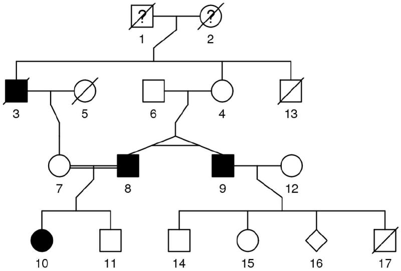
Four-generation pedigree plot with shapes for male (square), female (circle), and unknown gender (diamond). The shapes are shaded, un-shaded, or filled with a question mark (?) for disease status of yes, no, and unknown, respectively. A diagonal line is drawn through the shape of those who have deceased. Twins are represented as diagonal lines split from a single mating event with a horizontal line drawn to both horizontal lines indicating the twins are monozygotic. A consanguineous marriage is indicated by two horizontal lines connecting the parents rather than one.

Pedigree Trimming

Pedigree analyses are often based on a subset of pedigree members that are informative for a specific analysis. For example, subjects who are not genotyped and do not have offspring are not informative for linkage or association analyses, and can be trimmed from the pedigree. However, some uninformative subjects are needed to maintain links among relatives to maintain a valid pedigree. The pedigree.shrink function trims uninformative pedigree members while maintaining a valid pedigree structure down to a specific bit size, a metric used for allocating memory in some pedigree linkage analysis packages[7], defined as bit_size=(2*M)-N, where M and N are the number of non-founders and founders within the pedigree, respectively. For a more detailed description of the algorithm with a working example, see the Supplementary Material.

Kinship Matrices

The kinship coefficient for any two subjects is the probability that an allele chosen at random for both subjects at a given locus are identical-by-descent (IBD), that is, inherited from a common ancestor. The computations in the kinship function are based on a recursive algorithm described in Lange[8], which assumes the founders are not inbred. Kinship matrix K can be transformed to a genetic correlation matrix by 2*K, which can be used in mixed models to estimate the additive genetic effect of alleles on phenotype.

The kinship function is now able to calculate the kinship matrix for the X chromosome. The recursive algorithm accounts for the asymmetry of the X chromosome transmission between males and females. Males will have K_i,i = 1 for the X chromosome, whereas for females K_i,i is the same as for autosomes. The genetic correlation matrix for the X chromosome is 2*K_i,j for a pair of females, K_i,j for a pair of males, and (2^1/2)*K_i,j for a male-female pair. How the genetic correlations influence mixed models depends on assumptions of dosage compensation, that is, the amount of inactivation of one of the two X chromosomes in females[9]. Examples for both autosomes and the X chromosome are provided in the Supplementary Material.

We provide a framework to keep kinship matrices for multiple pedigrees in one object. A pseudo-code example for creating a kinship matrix from a pedigreeList object of multiple pedigrees is as follows. Given a data frame called “families” with multiple families indexed by the “pedid” variable:

R> pedlist <- with(families,
+ pedigree(id=sid, dadid=fid, momid=mid, sex=sex, famid=pedid))
R> kinmat <- kinship(pedlist)

The kinship matrix is symmetric and the kinship matrix for multiple families is block-diagonal with each family a block along the diagonal. The Matrix R package (Matrix.R-forge.R-project.org/) provides methods for efficient storage and manipulation of these sparse matrices. This is useful because the genetic correlation for related subjects in mixed models, as noted above, can be created using kinship matrices, which can be used with other covariance structures in modeling related subjects[10, 11]. Some simple tests on K replicates of the 17-member pedigree in Figure 1 give run time and storage of the kinship matrix of 1.2sec and 49Kb for 200 replicates, and 1.85s and 92Kb for 400 replicates, which is a linear increase on both measures; which are sufficient for most analyses.

DISCUSSION

We have highlighted the pedigree object and the core functions, plot.pedigree, pedigree.shrink and kinship. While other methods for pedigree analysis and plotting exist [3-5], these functions have few competitors within the R framework, where data management is built-in and methods have been written to use pedigree objects. These advantages make the routines in kinship2 suitable for studies where screening steps and analyses are performed across many families. We have made the kinship2 package available on the Contributed R Archives Network cran.r-project.org/web/packages/kinship2 with a vignette; we invite feedback and contributions.

References

- 1.Zhao JH. Pedigree-drawing with R and graphviz. Bioinformatics. 2006;22(8):1013–4. doi: 10.1093/bioinformatics/btl058. [DOI] [PubMed] [Google Scholar]
- 2.Therneau T, Grambsh P, editors. Modeling Survival Data: Extending the Cox Model. Springer-Verlag; 2000. [Google Scholar]
- 3.Fuchsberger C, et al. PedVizApi: a Java API for the interactive, visual analysis of extended pedigrees. Bioinformatics. 2008;24(2):279–81. doi: 10.1093/bioinformatics/btm577. [DOI] [PubMed] [Google Scholar]
- 4.Trager EH, et al. Madeline 2.0 PDE: a new program for local and web-based pedigree drawing. Bioinformatics. 2007;23(14):1854–6. doi: 10.1093/bioinformatics/btm242. [DOI] [PubMed] [Google Scholar]
- 5.Makinen VP, et al. High-throughput pedigree drawing. European Journal of Human Genetics. 2005;13(8):987–9. doi: 10.1038/sj.ejhg.5201430. [DOI] [PubMed] [Google Scholar]
- 6.Bennett RL, et al. Standardized human pedigree nomenclature: update and assessment of the recommendations of the National Society of Genetic Counselors. Journal of Genetic Counseling. 2008;17(5):424–33. doi: 10.1007/s10897-008-9169-9. [DOI] [PubMed] [Google Scholar]
- 7.Abecasis GR, et al. Merlin--rapid analysis of dense genetic maps using sparse gene flow trees. Nature Genetics. 2002;30(1):97–101. doi: 10.1038/ng786. [DOI] [PubMed] [Google Scholar]
- 8.Lange K, editor. Mathematical and Statistical Methods for Genetics Analysis. Springer; 1997. [Google Scholar]
- 9.Kent JW, Jr, Dyer TD, Blangero J. Estimating the additive genetic effect of the X chromosome. Genetic Epidemiology. 2005;29(4):377–88. doi: 10.1002/gepi.20093. [DOI] [PMC free article] [PubMed] [Google Scholar]
- 10.Schifano ED, et al. SNP Set Association Analysis for Familial Data. Genetic Epidemiology. 2012 doi: 10.1002/gepi.21676. [DOI] [PMC free article] [PubMed] [Google Scholar]
- 11.Schaid DJ, M S, Sinnwell JP, Thibodeau SN. Multiple genetic variant association testing by collapsing and kernel methods with pedigree or population structured data. Genetic Epidemiology. 2013;37(5):409–18. doi: 10.1002/gepi.21727. [DOI] [PMC free article] [PubMed] [Google Scholar]
Associated Data
This section collects any data citations, data availability statements, or supplementary materials included in this article.