Kinetic Quantitation of Cerebral PET-FDG Studies Without Concurrent Blood Sampling: Statistical Recovery of the Arterial Input Function

Abstract

Kinetic quantitation of dynamic positron emission tomography (PET) studies via compartmental modeling usually requires the time-course of the radio-tracer concentration in the arterial blood as an arterial input function (AIF). For human and animal imaging applications, significant practical difficulties are associated with direct arterial sampling and as a result there is substantial interest in alternative methods that require no blood sampling at the time of the study. A fixed population template input function derived from prior experience with directly sampled arterial curves is one possibility. Image-based extraction, including requisite adjustment for spillover and recovery, is another approach. The present work considers a hybrid statistical approach based on a penalty formulation in which the information derived from a priori studies is combined in a Bayesian manner with information contained in the sampled image data in order to obtain an input function estimate. The absolute scaling of the input is achieved by an empirical calibration equation involving the injected dose together with the subject’s weight, height and gender. The technique is illustrated in the context of ¹⁸F-Flu-orodeoxyglucose (FDG) PET studies in humans. A collection of 79 arterially sampled FDG blood curves are used as a basis for a priori characterization of input function variability, including scaling characteristics. Data from a series of 12 dynamic cerebral FDG PET studies in normal subjects are used to evaluate the performance of the penalty-based AIF estimation technique. The focus of evaluations is on quantitation of FDG kinetics over a set of 10 regional brain structures. As well as the new method, a fixed population template AIF and a direct AIF estimate based on segmentation are also considered. Kinetics analyses resulting from these three AIFs are compared with those resulting from radially sampled AIFs. The proposed penalty-based AIF extraction method is found to achieve significant improvements over the fixed template and the segmentation methods. As well as achieving acceptable kinetic parameter accuracy, the quality of fit of the region of interest (ROI) time-course data based on the extracted AIF, matches results based on arterially sampled AIFs. In comparison, significant deviation in the estimation of FDG flux and degradation in ROI data fit are found with the template and segmentation methods. The proposed AIF extraction method is recommended for practical use.

I. Introduction

Molecular imaging with dynamic positron emission tomography (PET) studies can be used to evaluate local biologic characteristics of tissue, in vivo. Comprehensive quantitation of dynamic PET data relies on kinetic modeling. However, most kinetic models require specification of an arterial input function (AIF) describing the activity of the radiotracer in the arterial supply to the tissue of interest [28]. In practice, there are situations where it is inconvenient or impossible to obtain this information by direct sampling. In a clinical setting, blood sampling by arterial catheterization necessitates specific technical expertise and additional complexities in laboratory practice. Moreover, such sampling generally adds to patient discomfort and may even introduce potential risks. With animal studies there are further issues of concern—small animals such as the mouse or rat have difficult vascular access and do not have the blood volumes necessary to make direct sampling feasible [17], [57]. Overall there is considerable interest in methods which enable blood information to be recovered with little or no direct sampling. Chen et al. [11] identified two general approaches to this problem, including 1) methods based on adaptation of the cardiac PET technique of Gambhir et al. [18] and 2) methods that are based on scaling of a population template blood curve derived from past experience with the radiotracer [14], [43], [49], [58]. Further studies based on representation of voxel-level PET time-course data via factor analysis models have also been considered [13], [34], [42], [56], [57], [63].

The focus in this work is on studies where the identification of an isolated arterial blood pool is problematic due both to the physical size of possible arterial pools in the field of view (i.e., scanner resolution) and to spillover contamination resulting from the high degree of tracer retention in surrounding tissue (kinetics of the radiotracer). Dynamic cerebral studies with FDG exhibit both these features. We propose a formulation that involves a synthesis of information derived from localized time-course data recovered at potential blood sources in the image volume and a priori statistical information derived from previous experience with the tracer. Although the identification of potential blood regions via co-registered imaging data [37] (MR or CT angiography) may sometimes be possible, it is of practical interest to have methods which can identify blood regions using the dynamic PET data only. Techniques based on cluster analysis [36] and segmentation [46] have potential. Here we propose a shape-driven segmentation technique that is guided by a novel cross-correlation of the image set with a historical template blood curve. Segmentation is also used to extract potential patterns of spillover contamination. Our work extends the familiar recovery-spillover formulation developed by Gambhir et al. [18] in the cardiac imaging context, to a more general context in which the contamination and recovery parameters affecting individual voxels are considered. The result is a mixture model representation of voxel-level time-course data within the blood region [46]. Components of variation in a historical database of a priori arterial blood curves are evaluated using a flexible parametric model. This model allows individual arterial blood curves to be represented as a parametric deformation of a reference template curve. The statistical distribution of the blood model parameters provides a basis for quantifying the types of curves which are consistent with past experience. This is a relevant source of information for specification of a blood curve in a new study. We develop a penalty based formulation that allows the synthesis of the information from the image data and the a priori blood curves. A statistical analysis of the relation between study (injected dose) and subject-level factors (gender, weight, height) and the scale of the arterial blood curve, provides an empirical approach to scaling the image-extracted input function without concurrent blood sampling.

The outline of the paper is as follows. Section II describes the methodology. Section III describes a study used for evaluation of the approach. The results are reported in Section IV. The paper concludes with some discussion.

II. Methodology

We begin with an overview of the approach. The problem is to estimate the AIF based on the acquired dynamic PET image data set and some supplementary concurrent information for the study (including dose and subject-specific variables such as height, weight, and gender). The image and supplementary information are symbolically denoted by z and x, respectively. We introduce a flexible family of AIF curves that are parameterized by a multidimensional shape parameter, θ, and a scale parameter, A. These AIFs are of the form AC_p(t|θ) for positive times, t. For any θ, the maximum of C_p(t|θ) is required to be unity, thus the scale parameter simply represents the maximum of the AIF. Conceptually, the AIF estimation problem is expressed symbolically as: given the information (x, z), recover the parameters (A, θ).

We propose a strategy in which the estimation of scale is based solely on the measured x-data, whereas the estimation of the shape uses both the x and z information. Historical studies (involving cases where the x-data and directly sampled AIFs have been simultaneously recorded), are used to develop the AIF representation and to characterize the statistical relation between the AIF scale and the x-information. This statistical relation is then applied to obtain a scale estimate for the data at hand; see Section II-D. There are a variety of reasons why a similar approach is not practical for the estimation of the shape of the AIF. While it is feasible to evaluate a simple historical relation between the x-data information and shape, incorporation of the image data is more complex. The excessive dimensionality, and indeed, the varying structure of the imaging information (e.g., variations in fields of view, resolution, physiology, etc.) restricts the ability to empirically describe the historical relation between the shape and the image data. The method pursued here involves modeling of the observed image data in terms of the shape and then combining that with a separate analysis of the statistical dependence of shape on the x-information. Thus, the approach is designed to choose a value for the AIF shape which is consistent with both image and historical information. There are a variety of ways in which this could be accomplished. If prior distributions for θ given x and sampling distributions for z given θ were available, then a standard Bayesian formulation could be applied [6]. But for reasons which will become clear below, this is not practical and as a result a more approximate Bayesian analysis based on a penalized likelihood-type formulation is used [23], [35]. Thus, we propose an estimator of θ which is defined as the minimizer of a cost (objective) function consisting of a linear combination of compliance to the image data (z) and the historical information (associated with x). The cost function is given by

$$l(\theta \mid x,z)=l_{\text{Image}}(\theta \mid z)+l_{\text{Historical}}(\theta \mid x)$$ (1)

where l_Image(θ|z) measures compliance to the image data and l_Historical(θ|x) measures compliance to the historical information. There is a rich theory that justifies consideration of such estimators [35], [60]. Indeed, many established approaches to parameter estimation, including methods for kinetic analysis in PET, can be formulated in these terms, e.g., [8]. Furthermore, a variety of PET image reconstructions based on filtered back-projection, the method of regularization and maximum a posteriori schemes can also be formulated in this way [23], [44], [50], [52]. Thus estimators resulting from the minimization of cost functions like l(θ|x, z) have a favorable pedigree. That is not to say that there is not a need to validate the utility of the approach in each new setting. This is a critical part of the current investigation; see Sections III and IV.

It should be appreciated that there are often a variety of ways to specify the functions l_Historical(θ|x) and l_Image(θ|z) in a penalty approach and still achieve very reasonable estimators. For example in the context of PET reconstruction a range of MAP and regularization estimators which correspond to quite different specifications for data fit and prior distributions, have been found effective. Our specification for the functions l_Historical(θ|x) and l_Image(θ|z) is developed in detail in Sections II-A and II-B. For the historical compliance we consider a set of feature vectors (functions), denoted by ψ_θ, and using multivariate regression tools [62] the conditional mean (μ_x = E[ψ_θ|x]) and covariance matrix (Σ_x = Var[ψ_θ|x]) of these features within the historical set are approximated. In terms of these quantities, the plausibility of an AIF shape (θ) is assessed by the Mahalanobis distance [40] of ψ_θ from μ_x, i.e., the quadratic form ${({\psi }_{\theta }-{\mu }_x)}^{\prime }{\mathrm{\sum }}_x^{-1}({\psi }_{\theta }-{\mu }_x)$. A mixture model [46] extension of the Gambhir et al. [18] spillover and recovery formulation used for extraction of blood curves from cardiac PET studies, is used to develop the image component, l_Image(θ|z), of the cost function. This is based on a weighted least squares deviation between voxel-level PET time-course measurements and their prediction based on the normalized AIF. Due to uncertainties with regard to what level of deviation to expect (i.e., the standard deviation of departures of data from model predictions), the least squares measure is integrated to obtain a criterion that is independent of this unknown standard deviation. This calculation, which is a standard Bayesian device [6], yields a factor proportional to the logarithm of a weighted residual sum of squares (WRSS) measure as our image data contribution to the cost function. Hence, the overall cost function for selection of θ and hence the AIF, is of the form

$$l(\theta \mid x,z)=\gamma log[\text{WRSS}(\theta )]+{({\psi }_{\theta }-{\mu }_x)}^{\prime }{\mathrm{\sum }}_x^{-1}({\psi }_{\theta }-{\mu }_x)$$ (2)

where γ has an interpretation as an effective degrees-of-freedom depending on dose, the frequency of temporal and spatial sampling and the spatial auto-correlation between voxels. If ψ_θ given x is approximately Gaussian then l_Historical(θ|x) can be viewed in Bayesian terms to define a prior distribution. Optimization of the cost function and its interpretation in more formal Bayesian terms is considered in Section II-C. The section ends with a description of a segmentation methodology for possible automated identification of blood pool regions within the image set. This can be useful in cases where the interactive identification based on anatomic knowledge of the tissue volume is not available.

A. Parameterization of AIFs and Construction of the Historical Penalty

A number of previous studies have found parametric representations to describe the behavior of the time-course of FDG activity in the arterial blood following a bolus injection into a peripheral vein [16], [20], [43], [58]. Both physiologically motivated and more empirical curve fitting techniques have been effective [38]. Although the methodology presented in this paper does not essentially depend on the particular form of parameterization used to represent blood curves, for demonstration purposes it is helpful to focus on a particular form. We consider a representation defined by a parametric manipulation or deformation of an adaptively defined reference population template. In this approach, we start with a fixed template curve, C̄_p(t), defined over a (spatial) domain [0, T] and create parametric variations by a series of manipulations designed to vary its shape without altering its uni-modal character. A specific construction for the template based on historical data is provided below, but let us suppose for now that the template is given. Assume C̄_p(t) for t ∈ [0, T] is normalized to have a maximum of unity and is uni-modal. For values of t outside [0, T], C̄_p(t) is simply extended by nearest-neighbor extrapolation (C̄_p(0) for t < 0 and C̄_p(T) for t > T). Let the location of the peak be denoted t̄_m. Deformation is achieved via four positive parameters (ρ, α_r, α_f, κ), denoted by a vector θ, that manipulate the location of the peak (ρ), the rise to and fall away from the peak (α_r, α_f) and the tail height (κ). For θ = (ρ, α_r, α_f, κ) and t_m(ρ) = T · (1+((T/t̄_m) − 1)/ρ)⁻¹ the deformed blood curve is given by

$$C_p(t\mid \theta )={\overline{C}}_p\left({\left[\frac{t}{t_m(\rho )}\right]}^{{\alpha }_r}{\overline{t}}_m\right)\text{for}0\le t\le t_m(\rho )$$

and

$$C_p(t\mid \theta )={\overline{C}}_p{\left({\overline{t}}_m+\left(1-{\left[\frac{T-t}{T-t_m(\rho )}\right]}^{{\alpha }_f}\right)(T-{\overline{t}}_m)\right)}^{\kappa }$$ (3)

for t ≤ t_m(ρ) ≤ T. C_p(t|θ) is evaluated outside of [0, T] by near-neighbor extrapolation. The deformed function has its maximum at t_m(ρ). Note t_m(ρ) is monotone increasing in ρ with t_m(1) = t̄_m and the limit of t_m(ρ) being either 0 or T as ρ tends to 0 or ∞. If θ = (1, 1, 1, 1) then C_p(t|θ) = C̄_p(t). The parameters α_r and α_f control the speed of the rise to and fall away from the peak. Since 0 ≤ C̄_p(t) ≤ 1, raising C̄_p(·) to the power κ, as indicated, manipulates the height of the tail. Some examples of blood curves achieved with different values of θ are shown in Fig. 1. Based on experience with collections of arterially sampled FDG blood curves, this simple model adequately represents components of variation [38]. Supporting data are presented in Section IV.

Fig. 1.

Illustration of the AIF model C_p(t|θ) [(3)] with different choices for θ = (ρ, α_r, α_f, κ). The solid black curve is the template C̄_p(t). (a) ρ = 0.25 (dashes) versus ρ = 4 (dots). (b) α_r = 0.25 (dashes) versus α_r = 4 (dots). (c) α_f = 0.5 (dashes) versus α_f = 2 (dots). (4) κ = 0.75 (dashes) versus κ = 1.5 (dots).

Historical Data: Template Definition and Measurement of Compliance

A set of historical blood curves for S subjects is an array, {(t_is, y_is); i = 1, 2, …, n_s; s = 1, 2, …, S}, giving the sampling times, t_is, in [0, T] and measured arterial activity values, y_is, for each curve. Note n_s represents the number of sampled points for subject s. The activity values can be normalized to have a maximum of unity and linearly interpolated at intermediate time-points so that the data set on subject can be viewed as defining a normalized curve $C_p^{(s)}(t)$ for t in [0, T]. In practice, measured arterial curves are also unimodal. We define the reference template curve, C̄_p, as the observed blood curve which, after adjustment for a time-shift (Δ) and scale (A), minimizes the overall misfit to the collection of historical curves. Thus, each one of the observed normalized curves, $C_p^{(s)}$ for s = 1, 2, …, S, is considered in turn as a possible template and residual sum of squares misfit to the collection of historical curves is calculated as

$$\text{RSS}(s)=\sum _{s^{\prime }=1}^S\left[\underset{\mathrm{\Delta },A}{min}\sum _{i=1}^{n_{s^{\prime }}}{\left[y_{i{s}^{\prime }}-{AC}_p^{(s)}(t_{i{s}^{\prime }}-\mathrm{\Delta })\right]}^2\right].$$ (4)

The final template is selected to be ${\overline{C}}_p-C_p^{(s^{\ast })}$ where s^* minimizes the residual sum of squares sequence {RSS(s) for s = 1, 2, …, S}. For fixed Δ, the optimization over A is a simple least squares computation. The optimization over Δ uses a simple grid-search—2-s steps over an interval ranging ±2 min is effective. For each s, these latter optimizations are required for each s′ in the inner sum in (4). The optimal template is found by enumeration of the S possible solutions in (4). Note in the highly unlikely event (this has never happened in our experience) that two or more curves yield the same minimum value for the cost function—we propose randomly choosing one of them as the template.

Given the template, C̄_p, each of the curves in the historical data set can be represented by a specific deformation. For the sth curve the scale (A_s) and shape (θ_s) are selected to minimize the residual sums of squares deviations between the data and the optimally shifted and parametrically deformed template, i.e.,

$$\text{RSS}(A,\theta )=\underset{\mathrm{\Delta }}{min}\sum _{i=1}^{n_s}{\left[y_{is}-A{\overline{C}}_p(t_{is}-\mathrm{\Delta }\mid \theta )\right]}^2.$$ (5)

Again the optimization over Δ uses a simple grid-search. For the optimization of RSS(A, θ) a standard nonlinear least squares optimization with numerical gradients is used [15]. Combining the scale and shape parameters with the associated set of supplementary x-information gathered for each study in the historical set yields a dataset {(A_s, θ_s, x_s) for s = 1, 2, …, S}. This dataset enables us to develop an understanding of the relation between the scale and shape and the x-information. This is a classical statistical regression problem [26]. By a variety of established classical and newer techniques, it is often possible to construct approximations for the conditional distribution of the output/response variable or some transformation of it (here scale or shape) in terms of the inputs/covariates (x-information). In the context of our own FDG dataset (see Sections III and IV), these analyses have led us to a feature vector consisting of the logarithmically transformed components of the shape parameter in combination with the logarithm of a contrast ratio (CR). The CR is defined as the ratio of the area under the AIF in a 5-min window 60 min after the peak to the area under the AIF in a 1-min period centered at the peak. Thus the feature vector used is ψ_θ = (log(ρ), log(α_r), log(α_f), log(κ), log(CR))′. The feature vector is found to be amenable to a simple linear representation of the conditional relation with the x-information. Specifically, we find

$$\begin{array}{l}E[{\psi }_{\theta }\mid x]={\mu }_x\approx {\beta }^{\theta }x\\ \mathit{Var}[{\psi }_{\theta }\mid x]={\mathrm{\sum }}_x\approx \mathrm{\sum }\end{array}$$ (6)

where β^θ is a coefficient matrix of dimension 5 × p (p is the row-dimension of the x-information and the superscript θ is to emphasize the relation to scale features) and Σ is a 5 × 5 covariance matrix. The Mahalanobis distance metric is used to assess the historical compatibility of a proposed value for the scale θ, i.e.,

$$l_{\text{Historical}}(\theta \mid x)={({\psi }_{\theta }-{\beta }^{\theta }x)}^{\prime }{\mathrm{\sum }}^{-1}({\psi }_{\theta }-{\beta }^{\theta }x).$$ (7)

Our analysis in Section IV finds that (ψ_θ − β^θx)′ Σ⁻¹ (ψ_θ − β^θx) is well approximated by a ${\chi }_5^2$ distribution. Remarkably, this would follow if the distribution of ψ_θ conditional on x were Gaussian [40]. With such an interpretation the historical compliance function could be viewed as twice the negative log-likelihood for ψ_θ conditional on x. Since the CR is necessarily a function of the AIF parameters, one might anticipate some inherent redundancy in the feature vector specification. This would indeed be the case if the elements of the feature vector were linearly related (they clearly are not). In general, the principal components [40] of the feature vector covariance matrix can be used to assess the degree of linear dependence among features (see Section IV). But it should be appreciated that over-elaboration of the feature vector is by no means problematic. In fact, by expressing the Mahalanobis distance in terms of the principal components of the covariance, one can see that it places the strongest emphasis on deviations from components that show the least variation. In the case that the feature vector had linearly dependent components, any proposed shape vector whose feature did not conform with this dependence, would have an infinitely large Mahalonobis distance. Hence, it would correctly be found to have unacceptable compliance with the historical data.

B. Modelling the Image Data Information

An approximate likelihood is also used to quantify the imaging data information. The image data consist of a set of N_B voxels corresponding to an approximate arterial blood pool region ( ) in the field of view of the PET scanner. The region could be user-defined or automatically identified by a suitable segmentation process; see Section II-E. The data in comprise of a collection of time-course vectors {z_ij, for j = 1, 2, …, J, and i = 1, 2, …, N_B}. The value z_ij is the PET measured radiotracer activity uptake in the j’th time-bin, [t_j, t̄_j) of data acquisition at the i’th voxel. The total number of time bins is J. Following a number of previous contributions to this topic, most notably Gambhir et al. [18], we model the activity using a 2-component scaled mixture of signals arising from the underlying blood source of interest and contaminating surrounding tissue. The blood component is of the form ${\mu }_j^B(\theta ,\mathrm{\Delta })={\int }_{{\underset{\_}{\mathrm{t}}}_j}^{{\overline{t}}_j}{C}_p(t-\mathrm{\Delta }\mid \theta )dt$ where Δ is a time-shift of the AIF. The need for this shift is to allow for the arrival of the AIF to the region . There may also be dispersion in the local arterial network but in the context of cerebral FDG kinetics the flow-related dispersion effects, which are on the order of 2–4 s [59], are not of practical importance, although accounting for dispersion is important with flow tracers. The tissue contaminant may vary depending on the voxel and is selected from a collection of possible patterns { ${\mu }_j^{[1]},{\mu }_j^{[2]},\dots ,{\mu }_j^{[L]}$, for j = 1, 2, …, J}identified by the user or by a segmentation process; see Section II-E. Thus, the final statistical model for the blood region of interest (ROI) data at the ith voxel is expressed as

$$z_{ij}=r_i{\mu }_j^B(\theta ,\mathrm{\Delta })+s_i{\mu }_j^{[l_i]}+{\epsilon }_{ij}$$ (8)

where the parameters r_i ≥ 0 and s_i ≥ 0 are recovery and spillover factors and l_i ∈ {1, 2, …, L}specifies the contaminating pattern most relevant to this voxel. Based on prior experience, we model deviations by ${\epsilon }_{ij}=w_{ij}^{-1/2}{u}_{ij}$ with u_ij approximately Gaussian with mean zero and constant variance [46]. However, one should appreciate that the pseudo-Poisson structure of PET uptake data limits the formal applicability of the Guassian except in areas with high tracer activity. The weight w_ij approximates the relative precision of z_ij; the variance of z_ij is approximately proportional to $w_{ij}^{-1}$. We set w_ij = w_i. w._j where $w_{i.}^{-1}=z_{i.}$ for $z_{i.}={\sum }_{j=1}^J{z}_{ij}$ the total uptake and $w_{.j}^{-1}$ is the sample variance of the proportional uptake pattern {z_ij/z_i., i = 1, 2, …, N_B} for j = 1, 2, …, J. Note that the temporal component of the weighting is consistent with a commonly used approach in fitting kinetic models to PET data [28]; the spatial structure reflects the pseudo-Poisson property of uptake (variance proportional to the mean). Theoretically, more efficient weighting schemes could be constructed but it is far from clear if such improvements can be practically realized in a finite sample setting. Indeed, the considerable experience with fitting techniques used in kinetic analysis of PET data would suggest that this is not a direction where significant improvements in efficiency could be achieved. A more extensive discussion of this issue is contained in O’Sullivan [46]. The weighted residual sums of squares achieved by optimal selection of the spillover, recovery and contamination factors is denoted WRSS_i = (θ|Δ) where

$$\begin{array}{l}{\text{WRSS}}_i(\theta \mid \mathrm{\Delta })=\underset{\{l_i,s_i,r_i\}}{min}\sum _{j=1}^J{w}_{ij}{\left[z_{ij}-r_i{\mu }_j^B(\theta ,\mathrm{\Delta })-s_i{\mu }_j^{[l_i]}\right]}^2\\ \equiv \sum _{j=1}^J{w}_{ij}{\left[z_{ij}-{\widehat{r}}_i{\mu }_j^B(\theta ,\mathrm{\Delta })-{\widehat{s}}_i{\mu }_j^{[{\widehat{l}}_i]}\right]}^2.\end{array}$$ (9)

The computation required is carried out using standard quadratic programming codes [46]. With further adjustment for the shift (Δ), the overall misfit of the model is assessed by the total weighted residual sum of squares

$$\begin{array}{l}\text{WRSS}(\theta )={min}_{\mathrm{\Delta }}\sum _{i=1}^{N_B}{\text{WRSS}}_i(\theta \mid \mathrm{\Delta })\\ \equiv \sum _{i=1}^{N_B}{\text{WRSS}}_i(\theta ).\end{array}$$ (10)

The approximation of weighted sums of squares statistics from linear and nonlinear models by scaled χ² or Gamma distributions is well established [6], [24], [35]. In the context of the normal weighted linear model the approximation is exact [62]. In view of this, at the true value of θ we might expect the distribution of the WRSS_i(θ)-values to approximately correspond to a scaled χ² distribution. Formally, if the Gaussian approximation were true, the degrees-of-freedom would be the number of time-points less the number of fitted parameters, i.e., 3 for the recovery, spillover, and contaminant pattern. Even though WRSS_i(θ)-values are spatially correlated, a histogram of these values permits the distribution to be assessed. Empirically (see Section IV) we find the scaled χ² distributions is applicable but the degrees-of-freedom (v_J) needs to be quite a bit less than the value of J − 3 which might be suggested by a naive Gaussian approximation. This is consistent with earlier work in the context of mixture models for PET data [46]. In our analysis, we allow v_J to be adapted based on observed WRSS_i(θ)-values. It is well-known that PET image reconstruction introduces spatial auto-correlation [9], [30], [39]. Assuming a first-order spatial auto-correlation between the WRSS_i(θ)-values measured at distinct voxels, the mean and variance of the misfit can be described by

$$\begin{array}{l}E[\text{WRSS}(\theta )]\simeq {\sigma }^2{\nu }_J{N}_B\\ \mathit{Var}[\text{WRSS}(\theta )]\simeq 2{\sigma }^4{\nu }_J{N}_B·\frac{1+\varphi }{1-\varphi }\end{array}$$ (11)

where σ²v_J ≃ E[WRSS_i(θ)] and ϕ is the voxel-to-voxel correlation coefficient, c.f. [46, Sec. 2].¹ Again, it is natural to approximate the weighted residual sums of squares by scaled χ² or Gamma distributions. The mean and variance of a Gamma Γ(a, b) distribution are ab and ab², respectively [6]. In view of this, we model the distribution WRSS(θ) by a Gamma distribution with parameters given by

$$a=\frac{{\nu }_J{N}_B(1-\varphi )}{2·(1+\varphi )}\text{and}b=\frac{2{\sigma }^2(1+\varphi )}{(1-\varphi )}.$$ (12)

The approximate Gamma distribution of the weighted residual sum of squares, suggests that for any σ we regard the image data information being evaluated by a likelihood of the form

$$\pi (z\mid \theta ,\sigma )\propto \frac{1}{b^a}exp\left(-\frac{\text{WRSS}(\theta )}{b}\right).$$ (13)

Thus, the information contained in the image data relating to the shape parameters (θ) will be assessed by −2log(π(z|θ, σ)) = 2(WRSS(θ)/b) + 2a log(b). Note that the likelihood in (13) is well calibrated in the sense that for fixed θ the optimal estimator of σ² based on maximization of this function is WRSS(θ)/(v_KN_B). This can be expected to be unbiased. The classical likelihood for a normal linear model based on N independent observations [62] would have a factor b^N/2 in place of b^a. Thus the likelihood function in (13) is defined to reflect that the effective degrees-of-freedom in the image data z is v_JN_B((1 − ϕ)/(1 + ϕ)) and not simply the product of the number of voxels (N_B) by the number of temporal samples (J). Intuitively, this is reasonable since the presence of auto-correlation should reduce the effective number of independent spatial elements from N_B to N_B((1 − ϕ)/(1 + ϕ)) and the pseudo-Poisson pattern should reduce the temporal contribution from J to v_J.

Unfortunately, the likelihood in (13) cannot be directly used without knowledge of σ². However, since σ² is determined by a range of factors including count rate, instrumentation (reconstruction methods) and biology, it is unlikely that its value can be reliably specified. In statistical terms, σ is a nuisance parameter. Uncertainty with regard to the value of σ limits the ability to directly use the weighted residual sum of squares in the cost function for determination of θ. A standard approach for dealing with this issue is to specify an a priori distribution for the nuisance parameter and use the resultant marginal posterior distribution to obtain inferences for parameters of interest; see Box and Tiao [6] for examples. In the present setting, employing Jeffery’s noninformative prior (∝ σ⁻¹) and integrating, the marginal likelihood becomes

$$\pi (z\mid \theta )=\underset{0}{\overset{\infty }{\int }}\pi (z\mid \theta ,\sigma )\pi (\theta )\frac{d\sigma }{\sigma }\propto \text{WRSS}{(\theta )}^{-a}.$$ (14)

Since compliance is expressed as two times the negative log-likelihood, we obtain

$$\begin{array}{l}{l}_{\text{Image}}(\theta \mid z)=2alog[\text{WRSS}(\theta )]\\ ={\nu }_J{N}_B\left(\frac{1-\varphi }{1+\varphi }\right)log(\text{WRSS}(\theta )).\end{array}$$ (15)

Note that in many contexts where Bayesian methods are applied, uncertainty with regard to the scale of the prior is treated in a fashion similar to the above. In particular, the derivation of the AIC [1] criterion is obtained in this way. The present situation is different because the prior information is fixed by the historical data and uncertainty is expressed with regard to the strength of the sample information (σ uncertainty).

C. Computation

Combining the historical and imaging data cost functions gives a criterion for estimation of the AIF shape parameters. Our proposed penalty-based AIF is ÂC_p(t|θ̂) where θ̂ is chosen to minimize

$$l(\theta )={\nu }_J{N}_B\frac{(1-\varphi )}{(1+\varphi )}log(\text{WRSS}(\theta ))+{({\psi }_{\theta }-{\beta }^{\theta }x)}^{\prime }{\mathrm{\sum }}^{-1}({\psi }_{\theta }-{\beta }^{\theta }x)$$ (16)

and  is defined in the next section. The optimization problem for θ̂ is simplified by consideration of the penalized weighted least squares cost function

$$l_{\gamma }(\theta )=\gamma \text{WRSS}(\theta )+{({\psi }_{\theta }-{\beta }^{\theta }x)}^{\prime }{\mathrm{\sum }}^{-1}({\psi }_{\theta }-{\beta }^{\theta }x)$$ (17)

for γ ≥ 0. Remarkably, the critical points (including the minimizer) of l(θ) can be obtained from the critical points of the penalized weighted least squares function. This is because with γ_θ = v_JN_B((1 − ϕ)/(1 + ϕ))WRSS(θ)⁻¹ we have

$${\partial }_{\theta }l(\theta )={\partial }_{\theta }{l}_{\gamma }(\theta ){\mid }_{\gamma ={\gamma }_{\theta }}.$$ (18)

For fixed γ, let θ̂_γ be the minimizer of l_γ(θ). The computation of the θ̂_γ-values is obtained by application of standard nonlinear least squares codes [15]. Formally, as WRSS(θ̂_γ) de-creases with increasing γ, the intersection of the line of identity (γ = γ), with the graph

$$\left\{\left(\gamma ,{\nu }_J{N}_B\frac{(1-\varphi )}{(1+\varphi )}\text{WRSS}{({\widehat{\theta }}_{\gamma })}^{-1}\right)\text{for}\gamma >0\right\}$$ (19)

identifies the value of γ, γ^* = v_JN_B((1 − ϕ)/(1 + ϕ))WRSS(θ̂_γ^*)⁻¹, for which θ̂_γ^* is the minimizer of the function l(θ). Alternatively a 1-D grid search of l(θ̂_γ) over γ >0 can be used to find the value (θ̂) which minimizes l(θ). Formally, the local uniqueness of critical points is a key consideration in any nonlinear optimization problem. In the present setting random transects of l(θ) in the neighborhood of (θ̂) is a practical diagnostic for assessment of this. More theoretical analysis based on fixed-point results require conditions on the higher order derivatives (see, for example, Cox and O’Sullivan [12]). The γ-values can be mapped into a probability scale by comparing (ψ_θ̂γ − β^θx)′Σ⁻¹(ψ_θ̂γ − β^θx) to the distribution of the corresponding Mahalanobis distances in the historical data. This provides an a priori assessment of the degree of compliance of with the historical data. Let p_γ be the observed frequency with which values of Mahalanobis distances exceed the value (ψ_θ̂γ − β^θx)′Σ⁻¹(ψ_θ̂γ − β^θx) in the historical data.

D. Scaling

Here, we model the relation between scale and the supplementary variables in the historical dataset {(A_s, θ_s, x_s) for s = 1, 2, …, S}. Our analysis finds a linear model for the logarithmically transformed scale to be reasonable, i.e.,

$$log(A_s)\simeq x_s^{\prime }\beta$$ (20)

where β is a p-dimensional regression coefficient and model deviations are mean zero with homogeneous variance [62]. It follows that the optimal mean square error estimator for the log-scale is log(A) = E[log(A)|x] = x′β. Thus if β̂ is the estimate of the regression coefficient from the historical data, the scale estimate for the current study is

$$\widehat{A}=e^{x^{\prime }\widehat{\beta }}.$$ (21)

Some Alternatives

In certain contexts [2], [18], it has been possible to model the structure of the recovery pattern and use it as a basis for scaling. Underlying these approaches is an assumption that it is possible to specify an arterial blood source, . Given and sufficient experience with the imaging system the recovery can be represented by a convolution between the assumed system point-spread, PS, and the indicator function ( ) for the source blood region. At the ith voxel we have

$${\widehat{r}}_i\simeq A·\text{PS}★I_{{\mathcal{R}}_O}[x_i].$$ (22)

Hence, the scale of an image derived blood curve could be un-biasedly estimated by a simple linear regression formula

$${\widehat{A}}_{\text{PS}}=\frac{{\sum }_{i=1}^{N_B}{\widehat{r}}_i{\ddot{r}}_i}{{\sum }_{i=1}^{N_B}{\ddot{r}}_i^2}$$ (23)

where r̈_i = PS ★ [x_i] are theoretical recovery coefficients. Often however, lack of specific knowledge of the relevant arterial blood source, , and perhaps to a lesser extent uncertainty in the system point-spread, limits the applicability of this technique. In our experience with cerebral FDG studies the approach has not shown promise; see the illustration in Section IV-B.

A further possibility might be to assume a recovery value for a collection of N_c voxels in the blood ROI. For example, if the average recovery over the set of voxels is expected to reach a value r̄_c, then an appropriate use of this information is to simply scale the image derived blood curve so that the estimated recovery is consistent with this expected value, i.e.,

$${\widehat{A}}_C=\frac{\frac{1}{N_c}{\sum }_{i\in C}{\widehat{r}}_i}{{\overline{r}}_c}.$$ (24)

This approach is readily extended to enable the image-derived blood curve to be scaled to achieve a desired value for any scale-dependent quantity, e.g., a blood volume or a flux over a normal tissue region in the field of view. However, the degree of confidence one might have in specifying a value for the reference (r̄_c) practically limits the objectivity of the approach.

E. Identification of the Blood ROI and Tissue Contaminant Patterns

Interactive user identification of relevant blood pools on the basis of imaging data is often difficult and time-consuming so an automated approach can have some practical utility. We apply a segmentation algorithm described in detail in O’Sullivan [46]. The method is based on a split-and-merge strategy and is designed to segment data on the basis of scaled time-course information. Voxel-level time-course data are scaled by the total uptake for the voxel. In statistical terms segmentation can be thought of as an adaptation/generalization of regression tree methodology [7] to the case where the independent variables in the regression are voxel coordinates and the dependent variable is a vector. If the voxel coordinate information is ignored, segmentation reduces to more classical cluster analysis [25]. There are many methodologies available for segmentation. The approach used is based on an adaptation of Bose and O’Sullivan [5] and Chen et al. [10]. First recursive splitting is used to reduce the tissue volume to a large number of boxes with the property that the data within each box has a high degree of homogeneity (low sums of squares deviation from the mean scaled time-course). This is followed by a merging process that recursively combines regions whose union leads to the smallest increase in regional inhomogeneity. Initial regions are the boxes produced by the splitting process; typically, this may be several thousand in number. There are two phases in the merging process. During the first phase regions are required to comprise of contiguous groups of voxels; in the second phase this constraint is relaxed and regions are allowed to be combined even if they are not adjacent. The motivation for the first phase is partially computational and partially because it tends to correctly identify components of tissue which are spatially contiguous and relatively homogeneous, such as sections of grey matter in the brain. The second phase provides the ability to capture more diffuse signals arising from isolated regions scattered throughout the tissue volume-signals from blood pools can be identified with the approach. Further details of the segmentation algorithm, including validation data are provided in O’Sullivan [46].

It is important to clearly appreciate that our segmentation scheme does not aspire to identify a collection of voxels that are in arterial vessels. Indeed in the case that the target volume only consisted of a single isolated arterial blood pool FBP reconstruction would typically lead to all voxels in the field of view having the same shaped time course, even though only a very few would actually correspond to arterial blood. Hence, in this hypothetical example, while our segmentation would try to include all voxels in subsequent analysis an alternative segmentation focusing on the arterial pool would entail consideration of a much more restricted (and noisy) collection of voxels. This is illustrated with the example in Section IV-B. Our segmentation method allows a subset of image voxels to be considered. We focus on voxels whose time-course pattern shows a strong cross-correlation with the template blood curve (C̄_p) defined in Section II-A above. Specifically, for each voxel we compute the R² statistic

$$R_i^2=1-\frac{{min}_{a,\mathrm{\Delta }}{\sum }_{j=1}^J{w}_{ij}{[z_{ij}-a{\overline{\mu }}_j^B(\mathrm{\Delta })]}^2}{{\sum }_{j=1}^J{w}_{ij}{[z_{ij}-{\overline{z}}_{i.}]}^2}$$ (25)

where ${\overline{\mu }}_j^B(\mathrm{\Delta })={\int }_{{\underset{\_}{\mathrm{t}}}_j}^{{\overline{t}}_j}{\overline{C}}_p(s-\mathrm{\Delta })ds$ for j = 1, 2, …, J. and z̄_i is the weighted average of the z_ij-values for j = 1, 2, …, J.. The segmentation algorithm focuses on the voxels with the largest R²-values (the top 10% are considered). The algorithm produces a collection of possible segments/regions (typically 3–4 because the number of voxels used is substantially limited). These regions could be examined interactively to identify a blood pool region but, by default, the region whose segmented time-course pattern shows the strongest cross-correlation with the template blood curve is used to define the blood region . An illustration of this is provided in Section IV-B.

Segmentation is also used to extract the patterns, {μ^[1], μ^[2], …, μ^[L], for l = 1, 2, …, L.}, representing contamination. Again the segmentation algorithm from O’Sullivan [46] is applied, but this time a different procedure is used to focus on voxels likely to include contamination sources. The voxels considered are ones which are in the proximity but not quite bordering the blood region. Let ϕ_h ★ [x] represent the convolution between the indicator function, , associated with the blood ROI and the 3-D Gaussian, ϕ_h, whose point-spread corresponds to the spatial resolution of the scanner. Note the total spillover at voxel x from the blood region is proportional to ϕ_h ★ [x]. Let G_FWHM(x) be the normalized convolution, ϕ_h ★ , scaled to have a maximum of unity. The set of voxels where the impact of spillover from the blood region is smaller than (ε > 0) is given by the set (ε) = {x : G_FWHM(x) < ε}. Let x^(k) be the image voxel corresponding to the k’th largest value of G_FWHM in (ε). We define an aura of the blood region with spillover threshold ε and N_A voxels by

$$A({\mathcal{R}}_B\mid \epsilon ,N_A)=\left\{x^{(k)}:k=1,2,\dots ,N_A\right\}.$$ (26)

In the case of cerebral FDG studies, values of ε = 0.001 and N_A = 4000 have been found effective, although the identified tissue contaminant signal is not found to be highly sensitive to these particular values (indeed a factor of 2 increase or decrease in ε or N_A did not influence results). Extraction of the tissue contaminants is based on segmentation of voxels in the blood region aura. The segmentation results in time-course patterns for each segment. The top (L = 4) patterns showing the least correspondence to the template blood curve are used to define the space of contaminators {μ^[1], μ^[2], …, μ^[L]}. Again the algorithm does not seem sensitive to the choice of L-values between 2 and 8 provide similar results.

III. Evaluation of the Approach: Study Details

¹⁸F-Fluorodeoxyglucose (FDG) is the most widely used radiotracer in PET [47]. When scanning is conducted in dynamic mode together with blood sampling, kinetic analysis can be applied to extract estimates of metabolic parameters related to the tissue’s consumption of glucose [47]. We consider a set of representative FDG studies from a 10-year period at the University of Washington. The data relate to cerebral PET_FDG studies in 91 human subjects; 79 of these were patients with disease (mostly cancer) and there are 12 subjects from a study of the cerebral glucose lumped constant in normals [22]. All studies involved catheterized blood sampling of a radial artery. We emphasize from the outset that our analysis finds no systematic differences between the blood curves of normal and nonnormal subjects; see Section IV-A. In the present validation, the nonnormal subjects are used for construction of an a priori distribution for arterial blood curves and for calibration of the scaling technique. Detailed evaluation of blood curve specification is carried out using the normal subjects. Three approaches to AIF specification without concurrent blood sampling are considered; (T) a fixed population template—the C̄_p curve as defined via (4), (S) a time-course produced by segmentation, and (P) a spillover and recovery adjusted curve produced by the penalty-based estimation technique—c.f. (16). All three curves are scaled using the empirical relation with dose and other study covariates (see Section II-D). The T, S and P AIFs are compared to the radially sampled AIF, denoted A, directly and also in terms of their impact on kinetic analysis. Relevant details of the data and the statistical methods used for comparisons are described here.

A. Data Acquisition

The studies involved a 1- or 2-min intravenous infusion of FDG radiotracer followed by dynamic PET imaging of the time-course of the radiotracer in the brain using a GE Advance scanner. Following injection, dynamic time-binned volumetric images of the radioactivity (measured in counts) were acquired over a 90-min time period. A total of 31 (J in the notation of Section II) time binned scans were obtained. Temporal sampling frequency varied throughout the 90 min: 1-min preinjection scan followed by 4 (15-s) scans, 4 (30-s) scans, 4 (1-min) scans, 4 (3-min) scans, and 14 (5-min) scans. Each scan provided a time-binned image volume with a total N = 128 × 128 × 35 voxels arranged on a regular lattice in transverse slices throughout the brain—35 (4.5 mm thick) planes with 128 × 128 (2.1 mm × 2.1 mm) pixels per plane. Blood sampling was carried out in all subjects using an automated blood sampler connected to an arterial catheter inserted into the radial artery. One-milliliter samples were obtained typically at 20-s intervals initially, followed by progressively longer intervals [20], [22]. The covariate (x-information) recorded for each study included: the injected dose, the duration of the bolus infusion, gender, age, height, weight, body surface area, and lean body mass index. In the normal subjects, regions of interest (ROIs) corresponding to eight structures within the grey matter (thalamus, caudate, parietal, frontal lobe, putamen, temporal lobe, cerebellum, and occipital cortex) as well as a white matter and whole brain regions were identified using co-registered MR scans [22]. FDG time-course data for each of the 10 ROIs in each of the 12 normal subjects were considered—120 data sets in all.

B. Historical Blood Curve Data Analysis

All arterially sampled blood curves are examined for conformity to the parameterized blood input function model. The best least squares fit of the model to the sampled arterial data is calculated for each curve. Weighted least squares fits are also considered but these are not found to impact any of our results. Restricting to the nonnormal studies, regression analysis is used to assess the relation between study covariates (x-values) and shape feature-parameters (ψ_θ), c.f. (6). A similar regression analysis is applied to analyze the relation between the logarithm of the scale and the study covariates, c.f. (20). In both cases, an all-subsets regression analysis is applied and only variables showing significant association with the response are retained. For any component of not included in the regression, the components of the coefficient values (β^θ, β) are simply set to zero. The deviations {ψ_θs − β^θx_s, s = 1. 2. … S} of the blood curve feature parameters adjusted for study covariates are examined in a variety of ways: 1) normal subject values are compared to non-normals using a repeated measures analysis of variance applied to the raw and ranked data [24] and 2) principal components [40] based on the sample correlation matrix of residual deviations are examined for approximate conformity to Gaussian assumptions. Specifically, the empirical distribution of the values of the quadratic form (ψ_θ − β^θx)′Σ⁻¹(ψ_θ − β^θx) (where Σ is the sample covariance matrix of the ψ_θ − β^θx deviations in the historical data) is evaluated for conformity to a ${\chi }_5^2$ distribution.

C. Assessment of Alternative Arterial Input Functions

In each study, four AIFs are available, labelled T, S, P, A above. We consider both direct and kinetic assessment of differences between these AIFs. Direct comparisons require timing and scaling adjustments. This is because the timing on the PET scanning and the blood sampling are not fully synchronized. Our comparisons take the radially sampled AIF(A) as the reference after it is first time-shifted (via kinetic modeling of whole brain time-course data as described below) to align with the period of PET data acquisition. Other AIFs are then aligned to the time-shifted radially sampled AIF. This approach allows deviations to be examined with an emphasis over the period of the PET data acquisition. Plots of the aligned curves are provided for each of the 12 normal studies.

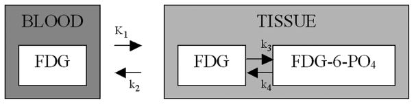
Kinetic comparisons between AIFs are based on the two-compartment FDG model [27], [48]; see Fig. 2. Time-course data from each ROI are modeled using each AIF to produce estimates of each of the four kinetic constants listed in Fig. 2 as well as a blood volume. This kinetic analysis uses standard weighted nonlinear least squares, e.g., Graham et al. [22]. For comparisons between different blood curves, we focus attention on a set of eight parameters ((K₁k₃/(k₂+k₃)), K₁, V_B, (K₁/(k₂+k₃)), k₃, (1/((k₂ + k₃)), (k₃/(k₂+k₃)), k₄). Aside from flow (K₁) and the blood volume(V_B), the parameters here represent: an FDG flux (K₁k₃/(k₂ + k₃)), a distribution volume estimate for glucose (K₁/(k₂ + k₃)), rates of phosphorylation (k₃) and dephosphorylation (k₄), a mean transit time for glucose(1/k₂ + k₃)), and an extraction fraction for glucose (k₃/(k₂ + k₃)). Note these eight parameters are selected for their established scientific relevance in the context of glucose and FDG [19]. With time-course data for the 120 ROIs the eight parameters are determined in each of four ways based on the alternative choices for the input function. This gives a total set of values for consideration. For each parameter, the combined set of 120×4×8 = 3840 values across the 12 normal subjects and 10 region combinations constitute a classic repeated-measures design [24], [41]. An overall analysis can be obtained using a linear model with effects for ROI and AIFs. For example, with the flux parameter if Flux_rsb denotes the flux value for region r and subject s using the AIF denoted by b, the linear model is

Fig. 2.

Two-compartment model for FDG [27], [48].

$${\text{Flux}}_{\text{rsb}}={\mu }_{rs}+{\zeta }_b+{\sigma }_E{\epsilon }_{\text{rsb}}$$ (27)

for r = 1, 2, …, 12, s = 1, 2, …, 10, and b = A, T, S, P. The errors (ε_rsb) are assumed to be independent with mean zero and unit variance. The parameter σ_E represents the pure error. For convenience, we set ζ_A = 0 so that the ζ_T, ζ_S, and ζ_P terms represent systematic deviations between flux parameters obtained using the template, segmentation and penalty estimated AIFs and the flux achieved using the radially sampled AIF. A direct estimate of these terms is obtained by averaging the within ROI differences of flux parameters obtained using T, S or P AIF and the flux obtained by the radially sampled AIF, i.e., for the template AIF we have

$${\widehat{\zeta }}_{\mathbf{T}}=\frac{1}{120}\sum _{rs}({\text{Flux}}_{rs\mathbf{T}}-{\text{Flux}}_{rs\mathbf{A}})$$ (28)

with analogous formulas for ζ̂_S and ζ̂_P. The statistical significance of these effects could be assessed using a simple paired t-test but to reduce the reliance on standard Gaussian error (ε_rsb) assumptions, a more robust paired Wilcoxon rank test is used [51]. The magnitude of the pure error [σ_E in (27)] provides a useful reference for evaluation of the practical importance of effects. The subject-to-subject variation in parameters, pooled across regions, is another useful reference. If the systematic effects are small relative to the pure error or the subject-to-subject variations, then they are likely to be of limited practical importance. The pure error is estimated by the linear model analysis; this is denoted by σ̂_E. We assess subject-to-subject variation using only the flux values calculated with the radially sampled AIF. Thus for each region we first compute the sample variance of the 12 flux values and then average these variances to obtain the overall subject-to-subject variation. We denote the square root of the subject-to-subject variation by σ̂_S.

The other components of the parameter set (K₁k₃/(k₂+k₃)), K₁, V_B, (K₁/(k₂+k₃)), k₃, (1/(k₂ + k₃)), (k₃/(k₂+k₃)), k₄) are treated in an identical way to the flux. Apart from these eight parameters, we also draw comparisons in terms of the fit of the kinetic model to the ROI time course data. The mean of the weighted squared deviations between the model fit and the data is used. To facilitate comparisons between parameters, systematic deviations and measures of variation are reported as percentage values relative to the average over the normal subjects of whole brain values for the parameter (computed using the radially sampled AIF). Thus, if μ̄_A is the whole brain average for a particular parameter, we report between subject and within ROI variation as well as the systematic deviations on a percentage scale, i.e., the fractional values (σ̂_S/μ̄_A, σ̂_E/μ̄_A, ζ̂_P/μ̄_A, ζ̂_S/μ̄_A, ζ̂_T/μ̄_A) expressed as percentages.

IV. Results

We begin by presenting results of the analysis of the historical blood curve data. Next, we present an illustration of penalty and segmentation AIF extraction for a normal cerebral PET-FDG study. This includes consideration of a number of relevant intermediates in the calculation, as discussed in Section II. The final part of this section reports a complete set of results for each of the 12 normal cerebral PET-FDG studies. The kinetic assessment of the accuracy of the three possible approximate AIFs (T, S, P) relative to the true radially sampled AIF (A) is presented.

A. Analysis of Historical Blood Curve Data

The collection of normalized arterial blood curves for FDG studies are presented together in Fig. 3(a). Note that even after adjusting for scale, there is substantial variability. Point-by-point normalized residual deviations of the optimized fixed template and deformed template [parameterized AIF in (3)] fits are summarized by box-plots in Fig. 3(b). These residuals, denoted $r_{is}^{FT}$ and $r_{is}^{DT}$ for the fixed and deformed template models, are defined by

Fig. 3.

(a) Normalized collection of 79 radially sampled arterial curves (grey). Residual deviations (points on the line at 0 activity) between normalized arterial curves and the optimized deformed template model [(3)]. The optimal fixed template fit shown in black. (b) Boxplots [51] of residual deviations from the fixed and deformed templates (28). (c) Principal components of the AIF model feature vectors (contrast ratio and four model parameters) adjusted for covariates (ψ_θ − β^θ x)-individual (vertical lines) and cumulative percent of variance explained (dashed line). (d) Histogram of the normalized Malhalanobis deviations, (ψ_θ − β^θ x)′Σ⁻¹(ψ_θ − β^θ x), over the 79 radially sampled arterial curves. Correspondence with quantiles of a scaled ${\chi }_5^2$ distribution (points)—line shows the idealized correspondence. 95% of Malhalanobis deviations are less than 15 (grey tick).

$$\begin{array}{l}{r}_{is}^{FT}=(y_{is}-{\overline{A}}_s{\overline{C}}_p(t_{is}-{\overline{\mathrm{\Delta }}}_s))/{\overline{A}}_s\\ r_{is}^{DT}=(y_{is}-A_s{C}_p(t_{is}-{\mathrm{\Delta }}_s\mid {\theta }_s))/A_s\end{array}$$ (29)

for i = 1, 2, … n_s and s = 1, 2, …, S, where (Ā_s, Δ̄_s) and (A_s, θ_s, Δ_s) are the optimized parameters for the respective fits [c.f. (4) and (5)] for subject. The four-parameter deformed template model (parametric AIF) represents a marked improvement over a fixed template. Due to its nonlinear nature, the four template adjusting parameters cannot be used to linearly predict the derived contrast ratio (CR)—a multiple linear regression model with the four blood model parameters only explains 57% of the variability in the contrast ratio. Thus the CR captures an additional component of variation which is not described by a linear combination of the four template adjusting parameters. Results of multiple linear regression of blood curve feature parameters (ψ_θ) on study covariates are presented in Table I together with the corresponding analysis for the logarithmic scale values (log(A)). The R² values for these regressions vary from 70% for the scale to 35% for the contrast ratio feature. Residuals from all analyses show substantial agreement with Gaussian assumptions. There is no theoretical reason for this behavior apart perhaps from the general tendency for many empirical measurements to approximately follow Gaussian laws. Regression parameter estimates (β^θ, β) and standard errors are reported in Table I. These values were computed by least squares but results showed only minor variations when computed using alternative robust regression techniques. Note the size of the standard errors is inversely proportional to the number of historical samples—cutting the historical sample in half would have the effect of increasing the standard errors by a factor of $\sqrt{2}$-roughly a 40% increase.

TABLE I.

Regression Models Relating Blood Curve Feature Parameters (ψ_θ) and Logarithmic Scale (A) to Study Covariates (S = 79 Cases). The Models Express the Response Variable as a Linear Combination of the Logarithm of the Listed Covariates. In the Case of Sex and Injection Duration Indicator Variables are Used. Estimated Model Parameters (Columns of (β, β^θ) and Standard Errors in Parentheses are Shown. Note Only Variables With a Significant Association With the Response are Used. Coefficient Values for Blank Cells are Zero. Median Values for Response and Covariates are Given. The Percent Error in the Model and Its R² Value are Provided

		log(A)	log(ρ)	log(αr)	log(αf)	log(κ)	log(CR)
Covariate (X)	Median	24.3	0.75	2.53	0.96	1.13	0.15
Dose (μ Ci)	9.51	0.96 (0.08)	-	-	-	-	-
Injection Duration (min)	1	0.06 (0.03)	0.17 (0.07)	1.05 (0.18)	0.33 (0.03)	−0.23 (0.03)	0.29 (0.04)
Sex Male vs Female	Male	−0.34 (0.02)	-	4.27 (1.3)	0.49 (0.19)	-	-
Height (cm)	175	–	-	104 (40)	13.8 (5.9)	-	-
Weight (kg)	78.3	5.31 (2.9)	-	-	-	-	-
LBM (lean body mass)	71.0	3.54 (1.9)	-	−41.8 (15.5)	-5.58 (2.31)	-	-
BSA (body surface area)	1.95	−13.4 (6.8)	-	-	-	-	-
Percent Error	-	14.3	31.9	84.0	12.5	13.8	19.7
R2	-	0.73	0.65	0.39	0.64	0.40	0.35

Principal components of AIF features adjusted for covariates, i.e., ψ_θ − β^θ x, are presented in Table II. Fig. 3(c) plots the percent variance explained as a function of the number of principal components. Roughly 90% of the total variance is explained by the first 3 components. As Table II shows over these components all five variables are strongly weighted—none of the individual variables can be ignored. The distribution of normalized Malhalanobis deviations, e.g., (ψ_θ − β^θ x)′Σ⁻¹ (ψ_θ − β^θ x), are found to show no significant deviation from a ${\chi }_5^2$-distribution—we obtain a p-value of 0.14 using a Kolmogorov–Smironov test [51]. Note this pattern would be expected if the individual deviations could be considered as a sample from a multivariate Gaussian distribution.

TABLE II.

Variance Components of Feature Vectors Adjusted for Covariate Information (ψ_θ − β^θx). Rows (Labeled PC) Present Loading Vectors for Principal Components of the Correlation Matrix of the Adjusted Features. Standard Deviations of These Principal Components are Labeled SD_pc [see Also Fig. 3(c)]; Standard Deviations of the Adjusted Features are Labeled SD_F

Adjusted Feature Vector (ψθ − βθ x)
	log(ρ)	log(αr)	log(αf)	log(κ)	log(CR)	SDPC
PC1	−0.15	−0.22	−0.48	0.57	0.61	1.50
PC2	−0.61	0.62	0.40	0.27	−0.12	1.21
PC3	−0.72	−0.62	0.08	−0.32	0.03	0.84
PC4	−0.29	0.38	−0.78	0.25	0.31	0.63
PC5	0.08	0.22	0.01	−0.66	−0.71	0.41
SDF	0.32	0.82	0.12	0.14	0.19

The covariate adjusted feature vectors for AIF shape as well as the corresponding deviations for the logarithmic scale [(6) and (19)] showed no systematic distinction between normals and nonnormal studies. Two sample analyses using either standard t-test or rank-based methods find no statistically significant mean differences between normals and nonnormals. An overall repeated measures analysis, jointly considering the feature deviations associated with blood curve parameters as well as corresponding deviations for the log-scale, also finds no significant differences between the structure of blood curves from nonnormal and normal subjects.

B. An Illustration

Details of the extraction of AIFs (T, S, and P) for a representative normal subject (labeled 9 in Fig. 6) are presented in Figs. 4 and 5.

Fig. 6.

AIF extracted from dynamic cerebral FDG studies in normal subjects (labeled 1–12). The radially sampled arterial AIF (red), penalty estimates AIF (P, black), segmentation AIF (S, blue dots) and the population template AIF (S, green) are shown. Curves are aligned to have their maximums coincide with the arterial curve and are normalized to have a maximum of unity.

Fig. 4.

Normal subject illustration (9 in Fig. 6). Left: The radially sampled arterial AIF (A, red), penalty estimate (P, black), template (S, green) and segmentation (S, pink). The spillover correction (averaged over all blood region voxels) is shown in blue. Right: FDG uptake (grey) on transverse, sagittal and coronal slices centered in the region of the blood ROI (pink) identified by segmentation. The aura of the blood ROI is indicated (blue).

Fig. 5.

Normal subject (9 in Fig. 6) illustration. (a) The penalty criterion in equation (15) (stars) and the weighted sums of squares in equation (9) (grey) and compliance with the historical records (circles)—l(θ̂_γ), WRSS (θ̂_γ) and p_γ—plotted as a function of the penalty parameter log(γ). (b) The distribution of the weighted residual sums of squares values, WRSS_i (θ̂) in equation (9), at the selected model. The points show the correspondence to a ${\chi }_{13}^2$ distribution. (c) Estimated scaled recovery coefficients compared to recovery coefficients obtained by convolution of the segmentation identified blood region with the point-spread of the resolution filter; see (r̂_i, r̈_i) in Section II-D. (d) Comparison between spillover and recovery coefficients, estimated values of s_i and r_i in equation (8). Correlation coefficients are indicated.

For this case the blood ROI identified by the segmentation algorithm is found to be substantially centered over a section of the left carotid artery. Transverse, sagittal and coronal slices of FDG uptake through the blood ROI are shown in Fig. 4. The aura of the blood ROI includes nearby sections of grey and white matter. Recall that the segmentation is based on shape characteristics of the observed time-course and not its absolute scale. As a result it is reasonable that voxels adjacent to the exact location of the carotid are included in the blood ROI. This is discussed at the beginning of Section II-E. While the segmentation blood curve shows some spillover contamination, the proposed analysis addresses this problem. The penalty extracted AIF is a very close match to the arterially sampled curve (Fig. 4). The average spillover adjustment is reminiscent of a typical decay-corrected FDG time-course associated with brain tissue. This is shown in Fig. 4. Further details of the analysis are provided in Fig. 5. The weighted residual sum of squares misfit, WRSS(θ̂_γ), plotted as a function of log(γ) shows improving fits to the image data are obtained with smaller values of the penalty parameter (γ). On the other hand, the degree of conformity to the reference distribution for arterial FDG curves increases with larger values of the penalty parameter. Note that conformity here is measured by the fraction of Malhalanobis deviations in the historical data, Fig. 3(d), that exceed (ψ_θ̂γ − β^θ x)′Σ⁻¹ (ψ_θ̂γ − β^θ x). From Fig. 5(a), the behavior of the cost function, (16), over the collection of AIFs parameterized by γ indicates a pattern which is consistent with a well-behaved quasi-convex cost function. There is no indication that the procedure used to compute the penalty based AIF should have difficulty. The penalty estimated AIF is in the 35th percentile of the distribution of historical AIFs. The conformity of the voxel level weighted residual sums of squares values, (16), to a scaled ${\chi }_{13}^2$ distribution is remarkably good [Fig. 5(b)]. No evidence of departure from the scaled ${\chi }_{13}^2$ distribution is found—a standard Kolmogorov–Smironov test [51] produced a p-value of 0.71. Note this is an important part of the assumption leading to the development of the penalty-based estimation criterion; see the discussion following (11). Our analysis estimates a degrees-of-freedom (v_J) for each study and different values (between 10 and 15) are found for the different studies. The correspondence between the estimated (r̂_i) and theoretical (r̈_i) recovery coefficients values obtained by convolving the indicator of the blood ROI with a 3-D Gaussian with a FWHM set to 6.5 mm, is shown in Fig. 5(c). Although there appears to be an approximate linear relation, the strength of this relation over voxels in the blood ROI is not impressive (R² = 0.61). The final plot in Fig. 5(d) shows the relation between spillover and recovery coefficients. As might be expected, higher spillover is generally associated with lower recovery.

C. Assessment of Approximate AIFs

The penalty estimated AIF for each of the normal subjects is shown in Fig. 6 together with the corresponding template and pure segmentation AIFs. Note that in this figure all curves are normalized to the same peak height. This facilitates comparison of curve shapes. Difficulties with the pure segmentation curves are most pronounced at late time points. In two studies (labeled 2 and 5 in Fig. 6), the injection of tracer actually preceded the initial 1-min scan. Remarkably, in spite of this, a reasonable AIF reconstruction is still obtained. Three cases, labeled 4, 7, and 12 in Fig. 6, show obvious deviation between the arterial and the template curves. Apart from these the fixed template is in good agreement with the radially sampled AIF. Deviations between the radially sampled AIF (A) and the three candidate AIF estimates (P, S, T) were computed. The median absolute deviations are the least for the penalty estimated AIF (P)—about 4 times smaller than the median deviations associated with the template AIF (T). Significantly larger deviations are obtained with the segmentation extracted AIF (S).

Results of the analysis of the 120 time-course data sets using the four alternative AIFs are presented in Figs. 7 and 8. With the exception of blood volume, kinetic parameters calculated on the basis of the penalty estimated AIFs are in close agreement with values obtained from the radially sampled AIF. Not surprisingly, the AIF obtained by scaling the segmentation, shows substantial deviation from the radially sampled AIF. This is particularly apparent for each of the scale-dependent parameters-flux, flow distribution volume and blood volume. But there are further problems for extraction and the de-phosphorylation parameters.

Fig. 7.

Flux (K₁k₃/(k₂ + k₃)), transport (K₁), blood volume (V_B) and volume of distribution (K₁/(k₂ + k₃)) parameters computed using the radially sampled (A), penalty (P), segmentation (S), and the template (T) AIFs.

Fig. 8.

Phosphorylation rate (k₃), mean transit time (1/(k₂ + k₃)), extraction fraction (k₃/(k₂ + k₃)) and de-phosphorylation (k₄) parameters computed using the radially sampled (A), penalty (P), segmentation (S), and the template (T) AIFs.

A detailed comparison between alternative kinetic analyses based on different AIFs is presented in Table III. After adjustment for individual ROIs, there are statistically significant average percent deviations between kinetic parameters produced by each of the arterial curves. Notably, in the case of the penalty and the template AIFs, the magnitude of the percent deviations are small in comparison to the measurement error (reported as the within ROI percent coefficient of variation in Table III) and in comparison to the between subject variation in the parameter values (between subject percent coefficient of variation in Table III). As noted above the fixed template approach shows a statistically significant deviation in the flux parameter. In the context of this tracer, where flux estimation is perhaps the key parameter of interest, this is certainly a concern. A more technical but also a more worrying concern is the behavior of the fit statistic. Relative to the radially sampled AIF, the template AIF produces significantly inferior fits to the ROI time-course data. In contrast, the data-fit with the penalty extracted AIF shows no systematic deviation from that achieved with the radially sampled AIF.

TABLE III.

Average (N = 12 Subjects) Whole Brain Values for Eight Metabolic Parameters Associated With the 2-Compartment FDG Model and the Quality of Fit to ROI Data (Based on the Root Mean Squared Residual). The Percent Coefficient of Variation in Parameter Values Between Subjects and Within ROIs are Shown. Average (Over 120 Data Sets—12 Subjects and 10 ROIs Per Subject) Percent Deviations Between Parameter Estimates Produced by Arterially Sampled Curves and Ones Produced by the Penalty (P), Segmentation (S), and the template (T) AIFs are given.

Parameter	Whole Brain Mean (μ̄A)	Coefficient of Variation		Deviations
		Between $\text{Subjects}(\frac{{\widehat{\sigma }}_S}{{\overline{\mu }}_{\mathrm{A}}})$	Within $\text{ROIs}(\frac{{\widehat{\sigma }}_E}{{\overline{\mu }}_{\mathrm{A}}})$	$\mathrm{P}(\frac{{\widehat{\zeta }}_{\mathrm{P}}}{{\overline{\mu }}_{\mathrm{A}}})$	$\mathrm{S}(\frac{{\widehat{\zeta }}_{\mathrm{S}}}{{\overline{\mu }}_{\mathrm{A}}})$	$\mathrm{T}(\frac{{\widehat{\zeta }}_{\mathrm{T}}}{{\overline{\mu }}_{\mathrm{A}}})$
$\frac{K_1{k}_3}{k_2+k_3}$	0.046	17	6	−2ns	16	−7
K1	0.097	21	18	−5ns	54	−11
VB	0.052	70	44	110	153	24ns
$\frac{K_1}{k_2+k_3}$	0.394	47	16	17	37	−13
k3	0.132	52	14	−15	−12ns	4ns
$\frac{1}{k_2+k_3}$	4.110	54	20	20	−8ns	−3ns
$\frac{k_3}{k_2+k_3}$	0.479	17	17	4ns	−55	6ns
k4	0.0098	34	14	11ns	40	16
FIT	0.011	70	23	2ns	12ns	27

Note in terms of the discussion in Section III, the Columns of the Table are μ̄_A and 100 × (σ̂_S/μ̄_A, σ̂_E/μ̄_A, ζ̂_P/μ̄_A, ζ̂_S/μ̄_A, ζ̂_T/μ̄_A). Except Where Indicated by ^ns, Deviations are Significant at the 0.01 Level

V. Discussion

We have developed a novel approach to the extraction of AIFs from dynamic PET imaging data. The method requires no concurrent blood sampling. The technique employes a penalty formulation which enables the information from a priori arterial blood curve data sets to be combined with the image data at hand. Thus, the approach can be viewed as a hybrid of a number previously defined techniques which have tended to separately concentrate on either imaging data or a priori blood curve information [11], [13], [14], [18], [63]. Our methodology provides the opportunity for blood regions to be specified by an automated segmentation tool that uses only dynamic PET image data as input. Thus the method can be applied in a more routine fashion by technical support staff who may not have detailed expertise in relevant vascular anatomy.

Our validation has focused on cerebral FDG studies in humans. Given the relatively small blood pools within the field of view and the high degree of FDG uptake in brain tissue (a consequently high degree of spillover), the extraction of blood curve information in this setting is challenging. We have emphasized a kinetic model assessment of extracted blood curves. In the context of FDG studies flux is usually the parameter of primary diagnostic significance, our consideration of other parameters provides a more detailed technical test of the accuracy of the AIF extraction technique. A further motivation for this comprehensive kinetic evaluation, is based on the fact that the FDG model is used more generally as a way to quantify dynamic PET data with a variety of other PET radiotracers.

While the present work has been substantially motivated by, and has been validated in, the context of cerebral FDG PET studies in humans, the methodology developed has potential applicability in many other settings where there is significant a priori data providing experience with the dynamics of the PET tracer in arterial blood. The adaptation and validation of the techniques developed here to other tracers and to other imaging contexts (including small animals) is currently being pursued.

Overall, the methodology developed in this paper has a potential to improve the level of kinetic information recovered by PET imaging in clinical and animal subject populations, where routine concurrent blood sampling is not practical.

References

- 1.Akaike H. A new look at the statistical model identification. IEEE Trans Autom Control. 1974 Dec;AC-19(6):716–723. [Google Scholar]
- 2.Asselin MC, Cunningham VJ, Amano S, Gunn RN, Nahmias C. Parametrically defined cerebral blood vessels as non-invasive blood input functions for brain PET studies. Phys Med Biol. 2004;49:1033–1054. doi: 10.1088/0031-9155/49/6/013. [DOI] [PubMed] [Google Scholar]
- 3.Bentourkia M. Kinetic modeling of PET data without blood sampling. IEEE Trans Nucl Sci. 2005 Jun;52(3):697–702. [Google Scholar]
- 4.Bentourkia M. Kinetic modeling of PET-FDG in the brain without blood sampling. Comput Med Imag Graph. 2006 Dec;30(8):447–451. doi: 10.1016/j.compmedimag.2006.07.002. [DOI] [PubMed] [Google Scholar]
- 5.Bose S, O’Sullivan F. A region based image segmentation method for multi-channel data. J Amer Statist Assoc. 1997;437:92–106. [Google Scholar]
- 6.Box GEP, Tiao GC. Bayesian Inference. Reading, MA: Addison-Wesley; 1973. [Google Scholar]
- 7.Breiman L, Friedman JH, Olshen RA, Stone CJ. Classification and Regression Trees. Belmont, CA: Wadsworth; 1984. [Google Scholar]
- 8.Byrtek M, O’Sullivan F, Muzi M, Spence AM. An adaptation of ridge regression for improved estimation of kinetic model parameters from PET studies. IEEE Trans Nucl Sci. 2005 Feb;52(1):63–68. [Google Scholar]
- 9.Carson RE, Yan Y, Daube-Witherspoon ME, Freedman N, Bacharach SL, Herscovitch P. An approximation formula for PET region-of-interest values. IEEE Trans Med Imag. 1993;12:240–251. doi: 10.1109/42.232252. [DOI] [PubMed] [Google Scholar]
- 10.Chen SY, Lin W, Chen T. Split-and-merge image segmentation based on localized feature analysis and statistical tests. Graph Models Image Process. 1991;53:457–475. [Google Scholar]
- 11.Chen K, Bandy D, Reiman E, Huang S-C, Lawson M, Feng D, Yun L-S, Palant A noninvasive quantitation of the cerebral metabolic rate for glucose using positron emission tomography, 18F-fluorodeoxyglucose, the patlak method, and an image-derived input function. J Cerebr Blood Flow Metabol. 1998;18:716–723. doi: 10.1097/00004647-199807000-00002. [DOI] [PubMed] [Google Scholar]
- 12.Cox DD, OSullivan F. Asymptotic analysis of penalized likelihood and related estimators. Ann Stat. 1990;18:1676–1695. [Google Scholar]
- 13.Chen K, Chen X, Renaut R, Alexander GE, Bandy D, Guo H, Reiman EM. Characterization of the image-derived carotid artery input function using independent component analysis for the quantitation of [18F] fluorodeoxyglucose positron emission tomography images. Phys Med Biol. 2007;52:7055–7071. doi: 10.1088/0031-9155/52/23/019. [DOI] [PubMed] [Google Scholar]
- 14.de Geus-Oei LF, Visser E, Krabbe P, van Hoorn B, Koenders E, Willemsen A, Pruim J, Corstens F, Oyen W. Comparison of image-derived and arterial input functions for estimating the rate of glucose metabolism in therapy-monitoring 18F-FDG PET studies. J Nucl Med. 2006;47:945–949. [PubMed] [Google Scholar]
- 15.Dennis JE, Jr, Schnabel RB. Numerical Methods for Unconstrained Optimization and Nonlinear Equations. Philadelphia, PA: SIAM; 2002. [Google Scholar]
- 16.Feng D, Wang X. A computer simulation study on the effects of input function measurement noise in tracer kinetic modeling with positron emission tomography (PET) Comput Biol Med. 1993 Jan;23(1):57–68. doi: 10.1016/0010-4825(93)90108-d. [DOI] [PubMed] [Google Scholar]
- 17.Ferl GZ, Zhang X, Wu HM, Huang SC. Estimation of the 18F-FDG input function in mice by use of dynamic small-animal PET and minimal blood sample data. J Nucl Med. 2007 Dec;48(12):2037–2045. doi: 10.2967/jnumed.107.041061. [DOI] [PMC free article] [PubMed] [Google Scholar]
- 18.Gambhir SS, Schwaiger M, Huang SC, Krivokapich J, Schelbert HR, Nienaber CA, Phelps ME. Simple noninvasive quantification method for measuring myocardial glucose utilization in humans employing positron emission tomography and fluorine-18 deoxyglucose. J Nucl Med. 1989 Mar;30(3):359–366. [PubMed] [Google Scholar]
- 19.Gjedde A. Does deoxyglucose uptake in the brain reflect energy metabolism? J Pharmacol. 1987;36:1853–1861. doi: 10.1016/0006-2952(87)90480-1. [DOI] [PubMed] [Google Scholar]
- 20.Graham MM. Physiologic smoothing of blood time-activity curves for PET data analysis. J Nucl Med. 1997;38(7):1161–1168. [PubMed] [Google Scholar]
- 21.Graham MM, Peterson LM, Hayward RM. Comparison of simplified quantitative analysis of FDG uptake. Nucl Med Biol. 2000;27(7):647–655. doi: 10.1016/s0969-8051(00)00143-8. [DOI] [PubMed] [Google Scholar]
- 22.Graham MM, Muzi M, Spence AM, O’Sullivan F, Lewellen TK, Link JM, Krohn KA. The fluorodeoxyglucose lumped constant in normal human brain. J Nucl Med. 2002;43:1157–1166. [PubMed] [Google Scholar]
- 23.Green PJ, Silverman BW. Nonparametric Regression and Generalized Linear Models: A Roughness Penalty Approach. London, U.K: CRC; 1994. [Google Scholar]
- 24.Hand DJ, Taylor CC. Analysis of Variance and Repeated Measures Multivariate. London, U.K: Chapman Hall; 1987. [Google Scholar]
- 25.Hartigan J. Clustering Algorithms. New York: Wiley; 1975. [Google Scholar]
- 26.Hastie T, Tibshirani R, Friedman J. The Elements of Statistical Learning: Data Mining, Inference, and Prediction. New York: Springer-Verlag; 2001. [Google Scholar]
- 27.Huang SC, Phelps ME, Hoffman EJ, Sideris K, Selin CJ, Kuhl DE. Noninvasive determination of local cerebral metabolic rate of glucose in man. Am J Physiol Endocrinol Metab. 1980;238:69–82. doi: 10.1152/ajpendo.1980.238.1.E69. [DOI] [PubMed] [Google Scholar]
- 28.Huang SC, Phelps ME. Positron Emission Tomography and Autoradiography: Principles and Applications for the Brain and Heart. New York: Raven; 1985. Principles of tracer kinetic modeling in positron emission tomography and autoradiography; pp. 287–346. 1986. [Google Scholar]
- 29.Huang SC, Wu HM, Shoghi-Jadid K, Stout DB, Chatziioannou A, Schelbert HR, Barrio JR. Investigation of a new input function validation approach for dynamic mouse microPET studies. Mol Imag Biol. 2004;6:34–46. doi: 10.1016/j.mibio.2003.12.002. [DOI] [PubMed] [Google Scholar]
- 30.Huesman RH. A new fast algorithm for the evaluation of regions of interest and statistical uncertainty in computed tomography. Phys Med Biol. 1984;29(5):543–552. doi: 10.1088/0031-9155/29/5/007. [DOI] [PubMed] [Google Scholar]
- 31.Iida H, Rhodes CG, de Silva R, Araujo LI, Bloomfield PM, Lammertsma AA, Jones T. Use of the left ventricular time-activity curve as a noninvasive input function in dynamic oxygen-15-water positron emission tomography. J Nucl Med. 1992 Sep;33(9):1669–1677. [PubMed] [Google Scholar]
- 32.Iida H, Miura S, Shoji Y, Ogawa T, Kado H, Narita Y, Hatazawa J, Eberl S, Kanno I, Uemura K. Noninvasive quantitation of cerebral blood flow using oxygen-15-water and a dual-PET system. J Nucl Med. 1998 Oct;39(10):1789–1798. [PubMed] [Google Scholar]
- 33.Jons PH, Ernst M, Hankerson J, Hardy K, Zametkin AJ. Follow-up of radial arterial catheterization for positron emission tomography studies. Hum Brain Mapp. 1997;5:119–123. [PubMed] [Google Scholar]
- 34.Lee JS, Lee DS, Ahn JY, Cheon GJ, Kim SK, Yeo JS, Seo K, Park KS, Chung JK, Lee MC. Blind separation of cardiac components and extraction of input function from H(2)(15) O dynamic myocardial PET using independent component analysis. J Nucl Med. 2001;42:938–943. [PubMed] [Google Scholar]
- 35.Lehmann EL. Theory of Point Estimation. New York: Wiley; 1983. [Google Scholar]
- 36.Liptrot M, Adams KH, Martiny L, Pinborg LH, Lonsdale MN, Olsen NV, Holm S, Svarer C, Knudsen GM. Cluster analysis in kinetic modeling of the brain: A noninvasive alternative to arterial sampling. NeuroImage. 2004;21:483–493. doi: 10.1016/j.neuroimage.2003.09.058. [DOI] [PubMed] [Google Scholar]
- 37.Litton JE. Input function in PET brain studies using MR-defined arteries. J Comput Assist Tomogr. 1997;21:907–909. doi: 10.1097/00004728-199711000-00012. [DOI] [PubMed] [Google Scholar]
- 38.Kirrane J. PhD dissertation. Univ. College Cork; Cork, Ireland: 2009. Statistical modeling of blood curves in dynamic PET FDG data. [Google Scholar]
- 39.Maitra R, O’Sullivan F. Variability assessment in PET and related generalized deconvolution problems. J Amer Statist Assoc. 1998;93:1340–1356. [Google Scholar]
- 40.Mardia KV, Kent JT, Bibby JM. Multivariate Analysis. London, U.K: Academic; 1997. [Google Scholar]
- 41.Nachtsheim CJ, Neter J, Kutner M, Wasserman W. Applied Linear Statistical Models. 5. New York: Irwin; 2006. [Google Scholar]
- 42.Naganawa M, Kimura Y, Ishii K, Oda K, Ishiwata K, Matani A. Extraction of a plasma time-activity curve from dynamic brain PET images based on independent component analysis. IEEE Trans Biomed Eng. 2005 Feb;52(2):201–210. doi: 10.1109/TBME.2004.840193. [DOI] [PubMed] [Google Scholar]
- 43.Olshen AB, O’Sullivan F. Camouflaged deconvolution with application to blood curve modeling in FDG PET studies. J Amer Statist Assoc. 1997;92(440):1293–1303. [Google Scholar]
- 44.O’Sullivan F. A study of least squares and maximum likelihood for image reconstruction in positron emission tomography. Ann Statist. 1995;23:1267–1300. [Google Scholar]
- 45.O’Sullivan F, Saha A. Use of ridge regression for improved estimation of kinetic constants from PET data. IEEE Trans Med Imag. 1999 Feb;18(2):115–125. doi: 10.1109/42.759111. [DOI] [PubMed] [Google Scholar]
- 46.O’Sullivan F. Locally constrained mixture representation of dynamic imaging data from PET and MR studies. Biostatist. 2006 Apr;7(2):318–338. doi: 10.1093/biostatistics/kxj010. [DOI] [PubMed] [Google Scholar]
- 47.Phelps ME. Positron emission tomography provides molecular imaging of biological processes. Proc Nat Acad Sci. 2000;97(16):9226–9233. doi: 10.1073/pnas.97.16.9226. [DOI] [PMC free article] [PubMed] [Google Scholar]
- 48.Phelps ME, Huang SC, Hoffman EJ, Selin Sokoloff L, Kuhl DE. Tomographic measurement of local cerebral glucose metabolic rate in humans with [F-18]2-Fluoro-2-deoxy-D-glucose: Validation of method. Ann Neurol. 1979;6:371–388. doi: 10.1002/ana.410060502. [DOI] [PubMed] [Google Scholar]
- 49.Philipp TM, Circiumaru V, Cardi CA, Thomas DA, Bal H, Acton PD. Simplified quantification of small animal [18F]FDG PET studies using a standard arterial input function. J Nucl Med Mol Imag. 2006;33(8):948–954. doi: 10.1007/s00259-006-0121-7. [DOI] [PubMed] [Google Scholar]
- 50.Qi J, Leahy RM. Resolution and noise properties of MAP reconstructions in 3D PET. IEEE Trans Med Imag. 2000 May;19(5):493–506. doi: 10.1109/42.870259. [DOI] [PubMed] [Google Scholar]
- 51.R Development Core Team. R: A Language and Environment for Statistical Computing. R Foundation for Statistical Computing; Vienna, Austria: 2008. [Google Scholar]
- 52.Silverman BW, Jones WC, Wilson JD, Nychka D. A smoothed approach to indirect estimation problems, with particular reference to stereology and emission tomography. J R Stat Soc B. 1980;52:271–324. [Google Scholar]
- 53.Silverman BW. Density Estimation for Statistics and Data Analysis. London, U.K: Chapman Hall; 1986. [Google Scholar]
- 54.Spence AM, Muzi M, Graham MM, O’Sullivan F, Krohn KA, Link JM, Lewellen TK, Lewellen B, Freeman SD, Berger MS, Ojeman GA. Glucose metabolism in human malignant gliomas measured quantitatively with PET, 1-[11C]glucose and FDG: Analysis of the FDG lumped constant. J Nucl Med. 1998;39:440–448. [PubMed] [Google Scholar]
- 55.Spence AM, Muzi M, Krohn KA. Molecular imaging of regional brain tumor biology. J Cell Biochem. 2002;39:25–35. doi: 10.1002/jcb.10406. [DOI] [PubMed] [Google Scholar]
- 56.Su KH, Wu LC, Liu RS, Wang SJ, Chen JC. Quantification method in [18F] fluorodeoxyglucose brain positron emission tomography using independent component analysis. Nucl Med Commun. 2005;26:995–1004. doi: 10.1097/01.mnm.0000184999.81203.5c. [DOI] [PubMed] [Google Scholar]
- 57.Su Y, Welch M, Shoghi K. The application of maximum likelihood factor analysis (MLFA) with uniqueness constraints on dynamic cardiac microPET data. Phys Med Biol. 2007;52(8):2313–2334. doi: 10.1088/0031-9155/52/8/018. [DOI] [PubMed] [Google Scholar]
- 58.Takikawa S, Dhawan V, Robeson W, Spetsieris P, Chaly T, Dahl R, Margouleff D, Eidelberg D. Noninvasive quantitative FDG/PET studies using an estimated input function derived from a population arterial blood curve. Radiology. 1993;188:131–186. doi: 10.1148/radiology.188.1.8511286. [DOI] [PubMed] [Google Scholar]
- 59.Vafaee M, Murase K, Gjedde A, Meyer E. Dispersion correction for automatic sampling of O-15-labeled H2 O and red blood cells. In: Myers R, Cunningham V, Bailey D, Jones T, editors. Quantification of Brain Function Using PET. San Diego, CA: Academic; 1996. [Google Scholar]
- 60.Wahba G. Spline Models in Statistics, ser. CBMS-NSF Regional Conference Series; Philadelphia, PA: SIAM; 1990. PA. [Google Scholar]
- 61.Wahl LM, Asselin MC, Nahmias C. Regions of interest in the venous sinuses as input functions for quantitative PET. J Nucl Med. 1999;40:1666–1675. [PubMed] [Google Scholar]
- 62.Weisberg S. Applied Linear Regression. New York: Wiley; 1985. [Google Scholar]
- 63.Wu HM, Hoh CK, Choi Y, Schelbert HR, Hawkins RA, Phelps ME, Huang SC. Factor analysis for extraction of blood time-activity curves in dynamic FDG-PET studies. J Nucl Med. 1995;36:1714–1722. [PubMed] [Google Scholar]
- 64.Wu HM, Huang SC, Allada V, Wolfenden PJ, Schelbert HR, Phelps ME, Hoh CK. Derivation of input function from FDG-PET studies in small hearts. J Nucl Med. 1996;37:1717–1722. [PubMed] [Google Scholar]