Application of neuroanatomical features to tractography clustering

Abstract

Diffusion tensor imaging allows unprecedented insight into brain neural connectivity in vivo by allowing reconstruction of neuronal tracts via captured patterns of water diffusion in white matter microstructures. However, tractography algorithms often output hundreds of thousands of fibers, rendering subsequent data analysis intractable. As a remedy, fiber clustering techniques are able to group fibers into dozens of bundles and thus facilitate analyses. Most existing fiber clustering methods rely on geometrical information of fibers, by viewing them as curves in 3D Euclidean space. The important neuroanatomical aspect of fibers, however, is ignored. In this article, the neuroanatomical information of each fiber is encapsulated in the associativity vector, which functions as the unique “fingerprint” of the fiber. Specifically, each entry in the associativity vector describes the relationship between the fiber and a certain anatomical ROI in a fuzzy manner. The value of the entry approaches 1 if the fiber is spatially related to the ROI at high confidence; on the contrary, the value drops closer to 0. The confidence of the ROI is calculated by diffusing the ROI according to the underlying fibers from tractography. In particular, we have adopted the fast marching method for simulation of ROI diffusion. Using the associativity vectors of fibers, we further model fibers as observations sampled from multivariate Gaussian mixtures in the feature space. To group all fibers into relevant major bundles, an expectation‐maximization clustering approach is employed. Experimental results indicate that our method results in anatomically meaningful bundles that are highly consistent across subjects. Hum Brain Mapp 34:2089–2102, 2013. © 2012 Wiley Periodicals, Inc.

INTRODUCTION

Diffusion tensor imaging (DTI) is a popular imaging modality for exploring brain circuitry in vivo by capturing water diffusion patterns in brain tissues. Water molecules are more likely to diffuse parallel along neural pathways, since myelin sheaths of axons act as barriers and restrict the mobility of water molecules along directions perpendicular to the neural pathways. In a DT image, each voxel records water diffusion pattern at a specific location of the brain using a second‐order tensor. The principal eigenvector of each tensor, corresponding to the maximal eigenvalue, indicates the major direction along which water molecules are diffusing. By tracing along these principal directions, neural tracts can be delineated via a process called tractography [Mori and Zijl, 2002].

In the literature, several fiber tractography algorithms have been proposed. A subset of these methods is summarized in Fillard et al. 2011 and Mori and Zijl 1999. An intuitive and straightforward approach traces the fiber streamline starting from a given seed point, following the directions corresponding to the principal eigenvectors of the tensors. Tracing continues until the streamline encounters regions where principal diffusion directions can no longer be reliably estimated (i.e., cortical regions with low FA values), or where a sharp turn has occurred on the fiber pathway and the curvature is too large. The tractography procedure above, when performed using all possible seed points in the brain space, can lead to a massive number of fibers, typically of order 10³ to 10⁶. Alternatives track fibers by allowing the front of the seeding area to evolve in the context of tensor fields, borrowing ideas from more advanced numerical implementations [O'Donnell et al., 2002; Parker et al., 2002a].

Fiber tractography provides an effective approach for visualizing and analyzing brain connectivity and hence has important value clinically [Ciccarelli et al., 2008; Yamada et al., 2009]. For instance, a DTI study involving patients with multiple sclerosis (MS) reveals that FA values in regions affected by lesions drop to a level lower than the normal unaffected regions [Filippi et al., 2001]. The difference between the patients and the normal controls can be analyzed at the level of whole brain connectivity with the help of fiber tractography [Lin et al., 2007; Pagani et al., 2005].

However, the task of analyzing fibers produced by tractography is nontrivial. The massive amount of fibers often renders subsequent analyses difficult and makes information provided by the fibers not immediately decipherable. One possible solution to this problem is to group the fibers into coherent bundles for easier analysis. In Wakana et al. 2007, for instance, 11 major bundles are parcellated using a multiple‐ROI protocol, where fibers passing through the same manually delineated ROIs and sharing identical pathways are grouped together into a single bundle. However, manual ROI labeling requires the raters to be significantly trained; the outcome will otherwise be affected by significant intrarater and inter‐rater variations. Moreover, manual delineation is time consuming and may not be practically feasible when dealing with large DTI datasets. Automated fiber clustering (or tractography clustering) is becoming more commonplace as an automated alternative to partition the fibers into bundles, each of which contains fibers with similar structural and functional characteristics.

Most existing fiber clustering methods belong to the category of geometry‐based approaches, which view neural fibers as a set of typical 3D curves in the brain space. In Ding et al. 2003, for example, point‐to‐point correspondences are first established between fibers. The correspondence ratio between fibers is maximized when the two fibers are identical and approaches zero if pairwise correspondence is minimal. The fiber correspondence ratio is then utilized in calculating the similarity between fibers. With these similarity measurements, a traditional clustering strategy can be easily applied to group fibers into several bundles. Similar ideas are also applied in other studies [Maddah et al., 2007, 2008a].

Jonasson et al. 2005 propose that similarity between fibers can be calculated by counting the number of voxels that two fibers are sharing. The idea is further extended by Klein et al. 2007, where contributions toward counting the similarity from two fibers are individually weighted and integrated along the shared pathway. Other approaches involve extracting features from the spatial distributions of fibers. In Brun et al. 2004, the feature vector representing each fiber incorporates the mean of coordinates of all points on the fiber, as well as the covariance of the coordinates in the 3D space. Alternative feature representations include B‐Splines [Maddah et al., 2005, 2006], polynomials [Klein et al., 2008], etc. Hausdorff distance, as well as several variants, has also been widely applied for fiber clustering [Corouge et al., 2004; Gerig et al., 2004; Maddah et al., 2008b; O'Donnell et al., 2006; O'Donnell and Westin, 2005, 2007; Zhang et al., 2008]. In general, the Hausdorff distance regards fibers as curves in 3D space and computes the upper bound of the minimal point‐to‐point distance between fibers. Once the Hausdorff distance of fibers is ready, conventional clustering methods can be applied to group fibers into target bundles.

A common limitation of geometry‐based approaches is that the neuroanatomical characteristics of fibers are often ignored. The anatomical roles of the resulting bundles from geometry‐based clustering are elusive, since only geometric information has been utilized in clustering. Incorporating neuroanatomical information could potentially yield more intuitive results. For this purpose, Maddah et al. 2005 applied an atlas with expert‐labeled individual bundles for fiber clustering. Based on this atlas, target fibers are labeled according to their similarities with the labeled bundles. Similar approaches are also employed [O'Donnell and Westin, 2005, 2007], though the atlases used are in a virtual high‐dimensional space instead of the real brain space. Specifically, given the Hausdorff distance between any pair of fibers, the atlas can be constructed by embedding the fibers in a virtual high‐dimensional space. These atlas‐based methods represent a step forward from previous geometry‐based approaches, since the bundles are now parcellated by neuroanatomical annotation information.

Alternative atlases reflecting brain connectivity patterns have also been introduced for fiber clustering, to take advantage of the fact that fibers are reflecting brain neural connectivity. The Talairach atlas, which contains structural ROIs, is warped to the space of the individual subject for grouping fibers into bundles according to the ROI pairs connected by fibers [Xia et al., 2005]. Fibers that are too short to connect any pair of ROIs are grouped into the bundles according to geometric distances. A similar connectivity based approach is adopted in Li et al. 2010 by combining ROI connectivity information and geometrical features hierarchically. In particular, fibers are first grouped into several classes based on their connections to the ROIs. Then those fibers in an identical class are further clustered according to the Hausdorff distance between any pair of them. The atlases used in the above approaches are automatically warped to the space of the input subject via image registration, to provide labeling information of ROIs for the individual subject.

In this article, we propose a novel fiber clustering scheme that leverages the rich information given by the fiber neuroanatomy. Specifically, whole‐brain tractography is first performed to reveal all neural pathways in the brain. Then, we parcellate the brain space by a set of ROIs, which are further diffused according to the tractography data. ROI diffusion allows for more robust determination on the relationship between the anatomical regions (as delineated by the ROIs) and the fibers. Based on the diffused ROIs, we compute for each fiber its associativity vector, which describes its connectivity pattern with respect to all ROIs. Each entry of the associativity vector is a fuzzy measurement representing the likelihood of a fiber being connected to a particular region in the set of ROIs. The associativity vector depicts the feature of the fiber and works as its unique “fingerprint.” A multivariate Gaussian mixture is then used to model each bundle based on the fiber associativity vectors, effectively grouping together fibers that are characterized by similar structural connectivity. An expectation‐maximization (EM) approach associated with the parametric bundle models is employed to determine the bundle membership of each fiber. Experimental results show that the proposed method achieves consistent clustering results across individual subjects, implying its potential for utility in large‐scale analysis of DTI data.

METHOD

The neuroanatomical features of fibers are characterized by their individual associativity vectors. In “Neuroanatomical Features of Fibers” section, we will first describe how connectivity information of each fiber with respect to a set of ROIs is embedded in its associativity vector. Then, in “Bundle Modeling and Clustering” section, we will describe the parametric model utilized for capturing the distributions of the associativity vectors of the fibers. We will also describe the EM‐based clustering approach used for clustering the fibers into bundles.

Neuroanatomical Features of Fibers

Fibers connect different anatomical regions of the brain, forming the connectivity pattern that describes brain circuitry. For example, the forceps minor contains terminal fibers that pass from the genu to the frontal lobes, resulting in a unique neural pathway for signal transmitting between the left and the right hemispheres. More bundles can be further defined and identified from the very large amount of fibers, based on their similar structural connectivity patterns in common. Therefore, according to the connectivity pattern, fibers can be clustered into different bundles, each of which contains only fibers of similar structural and functional behaviors. Meanwhile, the commons of all fibers in a certain bundle can be utilized for the representation of the bundle as well.

Prior to characterizing the connectivity patterns of fibers, a set of brain anatomies needs to be identified and annotated for the subject under consideration. An automatic labeling procedure is applied in our studies here. Specifically, we warp the “Eve” atlas [Oishi et al., 2009] (called atlas for brevity in the rest of the article) to the native space of each individual subject via elastic registration. The atlas contains a T1 image, a coregistered tensor field, and a set of manually delineated ROIs for important anatomical structures of the brain. We register the atlas to the subject space via HAMMER [Shen and Davatzikos, 2002] based on their individual T1 images after the necessary preprocessing (e.g., bias correction, skull‐stripping, and tissue segmentation). The deformation field estimated in image registration is utilized to warp the set of ROIs associated with the atlas to the subject space, and label the subject into various anatomical regions. HAMMER [Shen and Davatzikos, 2002] guarantees high precision especially in aligning gyri and sulci, which are important in analyzing the connectivity patterns of fibers with respect to cortical areas.

Suppose that M ROIs are identified in the space of the subject, we can thus define the associativity vector L _i = (ℓ_i1, ℓ_i2, ···, ℓ_iM) for fiber i, where the entry ℓ_ij measures the relationship between fiber i and the j‐th ROI. Ideally, entry ℓ_ij can be set to 1 if any segment of fiber i lies within ROI j, and left unset otherwise. The straightforward binary formulation of the associativity vector records whether or not a fiber is connected to certain ROI. It is capable to describe the connectivity pattern for the fiber in terms of a collection of brain anatomies, and thus has been widely accepted in related studies. However, the binary formulation would result in sparse associativity vectors, pose challenges in estimating fiber distances, and increase the tendency of the clustering algorithms being trapped in local minima. Moreover, fibers that are prematurely terminated a little short of reaching the ROI due to imaging noise and low FA values will also be penalized and not taken into account when determining the connectivity patterns. A significant amount of information might be lost especially when connectivity of fibers with respect to cortical regions is under focus, simply due to the fact that FA values in cortex are usually low. In view of this, we propose a fuzzy ROI spatial confidence map by diffusing the ROI along directions indicated by the fibers. In the next, we will introduce the ROI diffusion procedure and the resulting spatial confidence map, followed by fuzzy associativity vectors of fibers derived from the diffused ROIs.

ROI diffusion and spatial confidence map

An ROI, which corresponds to specific brain anatomy, is generally delineated by a certain regional volume bounded by a closed surface or interface. For fibers that penetrate the ROI surface, their anatomical relationship with respect to the ROI can be known with high certainty. However, the possibility that fibers might be prematurely terminated due to imperfect tractography cannot be fully ruled out. In fact, this is quite common especially in the adjacencies of the white matter and the gray matter, where FA values are sometimes low and force the tracking to abort. To reveal the relationship between fibers and brain anatomies more accurately, we allow ROIs to diffuse gradually to incorporate fibers whose ends are out of the ROIs prior to diffusion.

The ROI diffusion can be performed in various ways. For example, in our previous work [Wang et al., 2010], we have used an improved transportation equation to describe the ROI and simulated the diffusion in a classical level‐set method. For better speed performance and higher accuracy, we have adopted the fast marching algorithm [Sethian, 1996, 1999] for ROI diffusion in this article. In Figure 1a, for instance, the original ROI is labeled in dark red and is bounded by the interface marked by the green‐dashed curve. The ROI begins to diffuse from the starting time point t _s, following the upper‐left‐to‐lower‐right bundle, and ends at t _e when the latest interface is indicated by the red‐dashed curve. The enlargement of the region covered by the ROI allows us to compensate for the cases where fibers are terminated prematurely to reach the original interface (green‐dashed curve) of the ROI, as indicated by the 3 (of 5) relatively shorter fibers in Figure 1a. The quantitative measure of the relationship will be recorded as a specific entry in the associativity vector, with details in the following.

Figure 1.

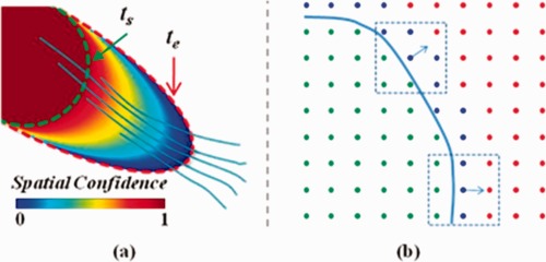
Illustration of the ROI diffusion example. (a) The ROI starts diffusing at t_s (green‐dashed curve) and terminates at t_e (red‐dashed curve), under the guidance of the upper‐left‐to‐lower‐right bundle. Five typical fibers are shown in the figure to represent the bundle. The procedure of ROI diffusion generates the spatial confidence map of the ROI according to the color bar provided. (b) Locations are labeled into three categories: green for inside, blue for active, and red for far‐away. ROI diffusion is always following the upwind normal directions (arrows) of the ROI interface (blue solid curve). [Color figure can be viewed in the online issue, which is available at http://wileyonlinelibrary.com.]

In the scenario of ROI diffusion based on fast marching, the interface of the ROI always propagates outward. In particular, locations which are already within the ROI interface are labeled “inside.” In Figure 1b, these inside locations are colored in green, while the light blue curve corresponds to the ROI interface. Certain locations out of the ROI are classified into the “far‐away” category (in red), if they are not neighboring to the evolving interface. The rest locations, though not incorporated by the ROI yet, are labeled “active” (in blue). The active locations are adjacent to the ROI interface and act as candidates to be part of the ROI, since any further perturbation of the interface are possibly to change them from active to inside immediately.

We further assume that the diffusion always follows the surface normal direction of the ROI interface, as indicated by the blue arrows in Figure 1b. The upwind diffusion direction for a specific location x on the interface, approximating the surface normal direction of the ROI interface at that location, is determined by connecting the mass center of inside locations and the mass center of all other locations (including both active and far‐away categories) in the neighborhood of x. The neighborhood in 2D is simply the 8‐connectivity as in the dashed rectangle of Figure 1b, while in 3D the 26‐connectivity. It is worth noting that the procedure described in the above is equivalent to that reported in Parker et al. [2001, 2002b].

The magnitude of the diffusion velocity is based on fibers generated by tractography. Suppose $\tau \left(x\right)\in [t_{\mathrm{s}},t_{\mathrm{e}}]$ represents the point of time at which the location x is traversed by the evolving interface and ν(x) for the diffusion speed at that location, the Eikonal equation [Sethian, 1996, 1999] should be satisfied as:

$$v\Vert {\nabla }_x\tau \Vert =1$$ (1)

For each location x on the ROI interface, the velocity of the ROI diffusion is defined by integrating contributions from all fibers passing x, where the contribution of each fiber equals the dot‐product of the tangent direction of the fiber at x and the interface normal direction at that location. Thus, given fibers traversing x and the collection of their tangent directions {d _a}, we have:

$$v\left(x\right)=\text{min}(V_{\text{max}},\sum _a{d}_a·\frac{v\left(x\right)}{\Vert v\left(x\right)\Vert })$$ (2)

Here, V _max is a predefined threshold regulating the maximal speed allowed in ROI diffusion. In our implementation, the value of V _max is set to 3, equivalent to that three fibers are passing the location x and the tangent directions of all fibers are parallel with diffusion direction.

The diagram of the algorithm for ROI diffusion is shown in Figure 2. In the beginning, the ROI interface incorporates inside locations only, as the diffusion is about to start from t _s. For initialization, the time values for locations outside the interface are unknown yet and set to infinity temporarily. The propagation of the ROI interface can only influence active locations immediately, where diffusion is allowed to happen. At each active location, the diffusion direction can be determined as soon as the ROI interface is about to reach that location, while the velocity is related to both the diffusion direction and fibers passing the location based on Eq. (2). Moreover, all active locations are pushed into a stack, which is further sorted in ascending order according to the estimated time points when the locations will be reached by the evolving interface. Then, in the next step, the active location in the top of the stack is popped out as the candidate to be incorporated into the ROI. The local patch of τ centered at the candidate location can be estimated according to Eq. (1), using the upwind stencil reported in Rouy and Tourin [1992]. In the following, as the ROI diffusion is progressing, the candidate itself is labeled inside and removed from the active stack. The far‐away locations in its neighborhood are now active and pushed to the stack. Also, the maximal τ of all inside locations indicates the progress of the ROI diffusion procedure. The value, denoted as τ′, will monotonously increase until reaching the end t _e, when the diffusion is supposed to stop, as the procedure is iterated.

Figure 2.

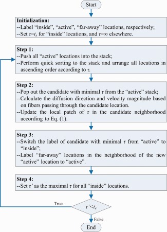
The major steps involved in ROI diffusion. [Color figure can be viewed in the online issue, which is available at http://wileyonlinelibrary.com.]

When ROI diffusion is completed, the procedure above will eventually output time values associate with individual locations, indicating when the locations are incorporated into the ROI in the progress of diffusion. For all locations, which are finally labeled as inside, the values of τ are distributed within the range [t _s, t _e]. We further invert the signs of all recorded time values and rescale them to the range of [0, 1], yielding the spatial confidence map of the ROI. In Figure 1a, for example, dark red indicates locations in the ROI prior to diffusion and dark blue indicates locations that are closer to the final interface when diffusion terminates, following the color coding for the spatial confidence of the ROI.

We have also provided a real example for ROI diffusion in Figure 3. The bundle connecting the left superior‐frontal gyrus (SPG‐L) to the right superior‐frontal gyrus (SPG‐R) is extracted and overlaid in red on the corresponding slice of the FA image in Figure 3a. The ROI of SPG‐L diffuses accordingly following the bundle, and results in the spatial confidence map in Figure 3b where the dark red area represents the initial ROI prior to diffusion. Similarly, the spatial confidence map of SPG‐R after ROI diffusion is computed and displayed in Figure 3c. Both (b) and (c) allow identical lengths of diffusion time and adopt the same color coding scheme of ROI spatial confidence map with that in Figure 1. It is obvious that the generated spatial confidence maps of both two ROIs in (b) and (c) are symmetric with respect to the sagittal plane as diffusion is guided by the same bundle of fibers in (a). Figure 3 is only an illustrative example for demonstrating the ROI diffusion process. For this reason, only the fibers in red are used to guide diffusion of ROIs. However, all fibers from whole‐brain tractography will be employed for ROI diffusion when applying our method to real data for fiber clustering.

Figure 3.

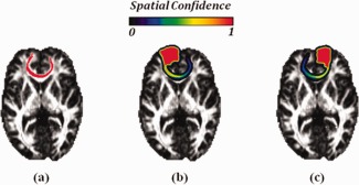
A real example of ROI diffusion. (a) The bundle connecting SPG‐L and SPG‐R are colored in red and overlaid on the FA slice. The resulted spatial confidence map of SPG‐L and SPG‐R after ROI diffusion following fibers in (a) are shown in (b) and (c), respectively. [Color figure can be viewed in the online issue, which is available at http://wileyonlinelibrary.com.]

Associativity vector for fiber modeling

As the spatial confidence map is available after the ROI has been diffused, the relationship between the fiber and the ROI can thus be determined even if the fiber is too short to enter the original region of the ROI. Given the set of ROIs, the associativity vector for each fiber under consideration is defined. For the associativity vector L _i of fiber i, the entry ℓ_ij is defined as the maximal spatial confidence value that fiber i comes upon the spatial confidence map of ROI j. The length of the associativity vector is thus equal to the number of ROIs employed. Moreover, since the spatial confidence map is a fuzzy description of the ROI after diffusion, the derived associativity vector is also a fuzzy measurement that is significantly different from the binary formulation introduced above.

To make possible fair comparisons of entries corresponding to different ROIs, the allowed lengths of diffusing time for different ROIs are set to identical. The value at a specific voxel on the spatial confidence map indicates the geodesic distance between the voxel and the original area of the ROI. Because of identical diffusion time, spatial confidence maps for individual ROIs are generated using the same unit. As the result, comparisons between different entries in the associativity vector and between two associativity vectors become meaningful. In general, the feature of each fiber can be described by its own associativity vector, which acts as the unique fingerprint signifying the connectivity pattern of the fiber with respect to individual brain anatomies. The associativity vectors will be further utilized to model different bundles, and for measuring the discrepancy between fibers.

The original Eve atlas consists of 130 ROIs, most of which are indicating anatomical structures of gyrus and sulcus. However, only 19 major bundles are targeted for fiber clustering in this article. To reduce the redundancy between entries of the associativity vector, we integrate smaller ROIs into larger ones, each of which has specific anatomical meaning. In particular, the complete list of ROIs used for generation of associativity vectors of fibers is provided in Table 1, where most ROIs are at the scale of lobe. Typical sagittal views of the ROIs are also overlaid on both corresponding T1 and FA slices in Figure 4 for better understanding. Note the annotations in Figure 4 have ignored the belongings of ROIs to two individual hemispheres. Note that the 7 ROIs shown in Figure 4 are from one hemisphere only and are half of the 14 total ROIs. It is also worth noting that the utilized ROIs are compatible with definitions of target bundles, which need to be identified by fiber clustering and will be discussed in the next section.

Table 1.

A total of 14 ROIs used for constructing the associativity vectors of fibers

Left frontal lobe	Right frontal lobe
Left central area	Right central area
Left occipital lobe	Right occipital lobe
Left parietal lobe	Right parietal lobe
Left temporal lobe	Right temporal lobe
Left subcortical area	Right subcortical area
Brainstem	Cerebellum

Figure 4.

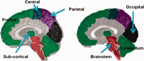
Sagittal views of the ROIs overlaid on T1 (left) and FA (right) images. [Color figure can be viewed in the online issue, which is available at http://wileyonlinelibrary.com.]

Bundle Modeling and Clustering

As mentioned previously, fibers with similar structural connectivity can be grouped together to form a bundle in common. According to Wakana et al. [2007], bundles can be defined based on regions which are connected by their member fibers. Therefore, fibers in the same bundle typically share similar neural pathways, and their associativity vectors should be highly correlated. In the other word, given fibers in a bundle as well as their associativity vectors, we are able to model the bundle by taking advantages of the neuroanatomical features of fibers. We further assume that the associativity vectors for all fibers within an identical bundle follow the distribution of a multivariate Gaussian mixture. Then an expectation‐maximization (EM) approach based on parametric bundle models can be used for fiber clustering. It is worth noting that other more complicated parametric models might also be applicable in modeling bundles. However, as shown in our later experiments, the Gaussian models of bundles can yield satisfactory results for fiber clustering.

To represent the bundle k using the multivariate Gaussian mixture, the parameters should include the mean associativity vector μ_k, which is related to the associativity vectors of all fibers contained in the bundle, and the corresponding covariance S _k. Recall the fact that spatial confidence maps of individual ROIs are generated within the same length of diffusion time. Therefore, μ_k and S _k can be easily acquired from the estimated associativity vectors of fibers. We further denote the associativity vector for fiber i (1 ≤ i ≤ N) as L _i and its membership to bundle k as ϖ_ik s.t. ${\sum }_k{\varpi }_{\mathrm{ik}}=1$. In the following, an EM‐based clustering method is employed for grouping fibers into individual target bundles. The EM‐based clustering framework typically consists of two iterative steps.

E‐step

According to Bayes rule, the membership of fiber i to bundle k can be estimated as:

$${\varpi }_{\mathrm{ik}}\leftarrow \frac{{\alpha }_k·N_k\left(L_i\right|{\mu }_k,S_k)}{{\sum }_{m=1}^K{\alpha }_m·N_m\left(L_i\right|{\mu }_m,S_m)}$$ (3)

where $N_k\left(L_i\right|{\mu }_k,S_k)$ gives the probability of L _i being sampled from the multivariate Gaussian distribution centered at μ_k with covariance matrix S _k. The term α_k corresponds to the normalized size of the bundle k, which will be further updated in the next M‐step. The membership ϖ_ik records the weighting factor of contribution from fiber i for calculating the parametric model of bundle k. In E‐step, the membership ϖ_ik, for fiber i to bundle k, is updated prior to the following M‐step.

M‐step

The model of bundle k and its corresponding parameters $({\mu }_k,S_k)$ are updated in the M‐step. Based on the latest membership ϖ_ik estimated in the previous E‐step, we first compute the mixture weighting factor for each bundle:

$${\alpha }_k\leftarrow \frac{{\sum }_{i=1}^N{\varpi }_{\mathrm{ik}}}{N}$$ (4)

The variable α_k here is simply the normalized size of each bundle, which has been utilized in Eq. (3). Then immediately we are able to update the parameters for models of different bundles:

$${\mu }_k\leftarrow \lambda {\mu }_k+\left(\frac{1-\lambda }{{\sum }_{i=1}^N{\varpi }_{\mathrm{ik}}}\right)\sum _{i=1}^N{\varpi }_{\mathrm{ik}}{L}_i$$ (5)

$$S_k\leftarrow \left(\frac{1}{{\sum }_{i=1}^N{\varpi }_{\mathrm{ik}}}\right)\sum _{i=1}^N{\varpi }_{\mathrm{ik}}(L_i-{\mu }_k){(L_i-{\mu }_k)}^t$$ (6)

In case, that drastic shifts of the mean associativity vector μ_k for bundle k might occur in iterative optimization due to the very abundant variation of fibers to be clustered, we have introduced an artificial argument λ into Eq. (5) and set the value to 0.95 to suppress the unexpected oscillation of μ_k.

Subsequent E‐steps and M‐steps will be iteratively executed until convergence, i.e., when the incremental change of the bundle models is insignificant, or the allowed number of iterations has been exhausted. Moreover, fibers with memberships that are lower than a predefined threshold are regarded as outliers and are discarded. To start the iterative procedure described above, proper initialization is required as it is critical to EM‐based clustering. We manually reproduce 19 major bundles in the atlas space to provide initialization for clustering, following protocol reported in Hofer and Frahm [2006] and Wakana et al. [2007]. The 19 bundles are listed in Table 2. They are selected as targets during fiber clustering due to the fact that all these bundles represent important connectivity structures in human brains and they are easily reproducible. Parameters (including the mean associativity vector and the covariance) for each manually delineated bundle are obtained and fed to the first E‐step as initialization. These parametric models in the atlas space will guide fiber clustering in each subject, while fibers of the subject will be either grouped into one of the 19 bundles or tagged as outliers.

Table 2.

The 16 target bundles

Abbreviations	Description
CST‐R	Right corticospinal tract
CST‐L	Left corticospinal tract
ATR‐R	Right anterior thalamic radiation
ATR‐L	Left anterior thalamic radiation
IFO‐R	Right inferior fronto‐occipital fasciculus
IFO‐L	Left inferior fronto‐occipital fasciculus
SLF‐R	Right superior longitudinal fasciculus
SLF‐L	Left superior longitudinal fasciculus
ILF‐R	Right inferior longitudinal fasciculus
ILF‐L	Left inferior longitudinal fasciculus
UNC‐R	Right uncinate fasciculus
UNC‐L	Left uncinate fasciculus
CB‐R	Right cingulum
CB‐L	Left cingulum
CCF	Corpus callosum connecting frontal lobes
CCC	Corpus callosum connecting central areas
CCO	Corpus callosum connecting occipital lobes
CCP	Corpus callosum connecting parietal lobes
CCT	Corpus callosum connecting temporal lobes

EXPERIMENTAL RESULTS

A total of 15 healthy subjects are used to evaluate the proposed fiber clustering method. The diffusion weighted data were acquired using a Siemens Allegra scanner (b = 2,000 s/mm², flip angle 90°, TR/TE = 13,640/82 ms, matrix 128 × 128, FoV 256 × 256 mm², slice thickness 2 mm, and 80 contiguous slices). The atlas with ROIs listed in Table 1 is warped to the individual space of each subject, to provide labeling information. As mentioned above, we perform registration via HAMMER [Shen and Davatzikos, 2002], as T1 data and tensor data for each subject have been coregistered already. Moreover, necessary preprocessing, including skull‐stripping and tissue segmentation of the T1 image, is performed for each subject for facilitating the warping of ROIs. Tractography is performed using FACT [Mori et al., 1999] with identical parameters across subjects.

In Figure 5, manually delineated bundles in the atlas space, following protocols in Hofer and Frahm [2006] and Wakana et al. [2007], are annotated in different colors. For all bundles in the left elliptical area of Figure 5, corresponding structures exist in both two hemispheres due to the reflectional symmetry with respect to the sagittal plane. However, only seven bundles from the identical hemisphere are displayed in the figure for clarity, while the other seven bundles are omitted here. The right part of Figure 5 represents the collection of corpus callosum fibers. These fibers pass through the sagittal plane as they are able to transmit signals between hemispheres. According to different anatomical regions connected by fibers, these corpus callosum fibers are further clustered into five bundles which are all shown in the figure. Therefore, we have specified 19 manually delineated bundles as the targets for clustering of fibers after whole‐brain tractography. Parametric models of these bundles in the atlas space are feed as initialization for the clustering process, as discussed in Bundle Modeling and Clustering section. It is worth noting that no limitation on the number or the composition of target bundles has ever been assumed in our method. Given different target bundles as initialization, our clustering method is capable to detect the corresponding bundles for each new subject.

Figure 5.

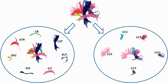
Target bundles in the atlas are shown and annotated. For simplicity, only bundles from the left hemisphere are provided in the left ellipse. The right ellipse contains the corpus callosum fibers, which are grouped into five bundles. There are a total of 19 manually delineated target bundles in the atlas space. [Color figure can be viewed in the online issue, which is available at http://wileyonlinelibrary.com.]

Visualization of Clustering Results

The proposed clustering method is performed independently on each of the 15 testing subjects. We randomly select four subjects and display the clustering results in Figure 6, which adopts the same color coding scheme for individual fiber bundles and drawing perspective with Figure 5. Each row of Figure 6 corresponds to a specific subject. The left column of Figure 6 shows all 12 bundles as in Figure 5. For clarity, we show only bundles that correspond to the left elliptical area of Figure 5 in the right column of Figure 6. The rest of the fiber bundles related to corpus callosum are depicted in the central column of Figure 6.

Figure 6.

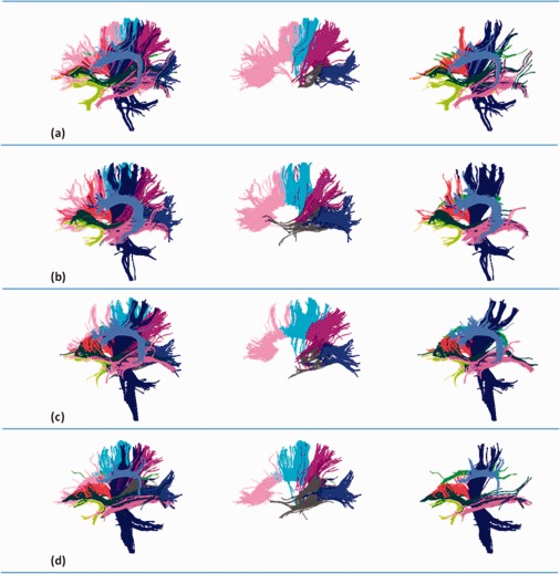
Clustering results from four randomly selected subjects. Each row corresponds to one subject. The same color coding scheme as Figure 5 is used here for rendering of the individual bundles. Similarly, 12 bundles are displayed in the left column. The corpus callosum bundles (middle column) are shown separately from the other bundles (right column) for clearly visualization. [Color figure can be viewed in the online issue, which is available at http://wileyonlinelibrary.com.]

For the four subjects in Figure 6, all target bundles have been identified, though some bundles are not shown here for convenience. The appearances of corresponding bundles (referring to the same color) are similar for each subject and the atlas. Therefore, we can conclude that the clustering results of these selected subjects are consistent with each other as well as the atlas. We will show next that the clustering results are consistent within the complete collection of all 15 subjects.

Connectivity of Fiber Bundles

Fibers in the same bundle behave similarly in terms of connectivity with respect to individual anatomical ROIs. Since the proposed clustering scheme is established on the connectivity patterns of individual bundles, we thus are able to investigate the connectivity behavior of fibers from the same bundle, which is identified via fiber clustering. To prove that the fiber clustering method is applicable to analyses of fibers and bundles, corresponding bundles of different subjects should have similar associativity vectors and behave consistently for connectivity patterns.

The associativity vectors tell connectivity patterns of fibers in a more accurate way with respect to the 14 ROIs listed in Table 1. For bundles that are restricted within a single hemisphere (the left elliptical area of Fig. 5), in particular, we are interested in connectivity patterns within the specific hemisphere only. For instance, CST‐L bridges cortical areas in the left hemisphere to the spine via the brainstem. Therefore, investigation of the connectivity patterns of CST‐L fibers should be focused on neuroanatomical areas in the left hemisphere only. We thus discard the associativity vector entries that are related to the other hemisphere and define the rest entries to form the partial associativity vector. The partial associativity vector neglects the difference between cortical/subcortical areas in the left/right hemispheres, and thus provides possibility to compare CST‐L and its counterpart CST‐R. We determine the partial associativity vectors for all fiber bundles, except those belonging to the corpus callosum. Entries in the partial associativity vector follow this order: frontal lobe, central area, parietal lobe, occipital lobe, temporal lobe, subcortical area, brainstem, and cerebellum. This order will be used in Figures 7, 8, 9.

Figure 7.

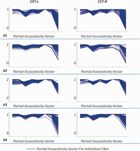
The partial associativity vectors for CST‐L and CST‐R from four randomly selected subjects. The blue curve indicates the partial associativity vector for each fiber. [Color figure can be viewed in the online issue, which is available at http://wileyonlinelibrary.com.]

Figure 8.

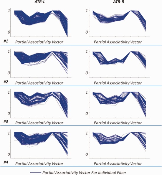
The partial associativity vectors for ATR‐L and ATR‐R from four randomly selected subjects. The blue curve indicates the partial associativity vector for each fiber. [Color figure can be viewed in the online issue, which is available at http://wileyonlinelibrary.com.]

Figure 9.

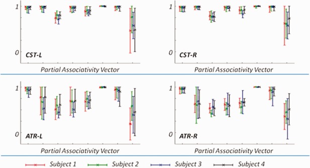
The mean partial associativity vectors, as well as the standard deviations, for selected bundles (including CST‐L, CST‐R, ATR‐L, and ATR‐R). The different colors mark the four individual subjects listed in Figures 7 and 8. Note that the maximal value of the associativity vector is restricted to 1. [Color figure can be viewed in the online issue, which is available at http://wileyonlinelibrary.com.]

In Figure 7, we plot the partial associativity vectors (in blue curves) of fibers in CST‐L and CST‐R from four individual subjects. In the figure, each row corresponds to a single randomly selected subject. The two columns are for CST‐L and CST‐R, respectively. For each subject, the high similarity of partial associativity vectors of fibers from the same bundle implies the consistency of fibers within the bundle. Moreover, connectivity patterns of fibers in either CST‐L or CST‐R, in terms of the partial associativity vector, are very similar across all the four selected subjects. This observation indicates that the clustering results are consistent across subjects. The interhemispheric symmetry can also be well observed by comparing the two columns in Figure 7, as the partial associativity vectors of CST‐L are very close to their counterparts of CST‐R.

n Figure 8, we plot the partial associativity vectors for ATR‐L and ATR‐R from the same four subjects as in Figure 7. The left column in Figure 8 is for ATR‐L, while the right column is for ATR‐R. In human brain, ATR indicates neural tracts that are neighboring and anterior to CST. However, the two families of fibers can still be differentiated according to their connectivity patterns. The plotted partial associativity vectors in Figure 8 confirm the difference of the connectivity patterns between ATR and CST (in Fig. 7), which validates that these bundles can be separated by utilizing the neuroanatomical features of fibers to clustering. We can also observe the interhemispheric symmetry between ATR‐L and ATR‐R for each individual subject. Also, the clustering results are consistent across all four subjects. The mean partial associativity vector and the corresponding standard deviation, for each of the bundles reported in Figures 7 and 8, is calculated and plotted in Figure 9. The results clearly indicate that, despite of the intersubject variability, clustering results are consistent across subjects.

For corresponding bundles of individual subjects, we are able to investigate the consistency of clustering results. For each bundle from a certain subject, we calculate the mean of the Pearson correlation coefficient of associativity vectors between all fiber pairs. The mean correlation coefficients for individual subjects are expected to be highly consistent, in that the corresponding bundles should behave similarly in connectivity patterns. We further average the mean correlation coefficients of the same bundles across all 15 subjects, and show the mean value as well as standard deviation in Table 3. In most bundles, the very high correlation scores indicate that fibers from a detected bundle are highly consistent. The low standard deviation confirms that the neuroanatomical patters associated with corresponding bundles from different subjects are compactly distributed. These properties of the clustering results achieved are important in related studies. For example, correspondence between identical bundles of different subjects can thus be established, which can work as constraints in image registration or segmentation. Moreover, population‐based analysis would be enabled given reliable and consistent correspondences between individual subjects.

Table 3.

The mean correlation of associativity vectors, as well as the standard deviation, across all 15 subjects

Bundle	Correlation
CST‐R	0.867 ± 0.021
CST‐L	0.906 ± 0.020
ATR‐R	0.898 ± 0.022
ATR‐L	0.926 ± 0.019
IFO‐R	0.924 ± 0.008
IFO‐L	0.935 ± 0.032
CB‐R	0.946 ± 0.020
CB‐L	0.924 ± 0.034
SLF‐R	0.976 ± 0.009
SLF‐L	0.953 ± 0.010
ILF‐R	0.943 ± 0.015
ILF‐L	0.939 ± 0.030
UNC‐R	0.969 ± 0.009
UNC‐L	0.975 ± 0.013
CCF	0.911 ± 0.035
CCC	0.934 ± 0.017
CCO	0.862 ± 0.021
CCP	0.857 ± 0.014
CCT	0.831 ± 0.037

DISCUSSION

We have proposed a complete framework to group fibers yield by whole‐brain tractography into 19 target bundles. To achieve this goal, 14 ROIs corresponding to different brain anatomies at the scale of lobe are utilized for the construction of associativity vectors of all fibers. The target bundles are defined following popular protocols reported in the literature. The selection of ROIs is determined by the target bundles simultaneously, as the ROI scale is compatible with the target bundles. For example, we partition corpus callosum into five bundles according to connected anatomies, which are in the list of ROIs applied. However, the application of the proposed method is not limited to the reported 19 target bundles only. Given other sets of target bundles and selected neuroanatomical descriptors in terms of ROIs, our method should be able to produce different but reasonable results.

In our framework, a critical step in calculating the features of the fibers is ROI diffusion. It is common to apply tensors directly for guiding simulated diffusion in studies on brain connectivity (i.e., tractography). However, since our main purpose in this work is to characterize the associativity between the fibers and a set of ROIs, it is more straightforward to use the fibers to guide the diffusion. This will (1) avoid accidental diffusion into regions of low anisotropy, and hence (2) speed up computation by avoiding unnecessary diffusion into unwanted regions.

We choose to use the maximal spatial confidence to form the associativity feature vector of each fiber to help avoid the negative influences caused by imperfections of the tractography algorithm. Because of the greedy nature of the tractography algorithm, the resulting fibers will sometimes be longer or shorter. We hence choose not to rely on the spatial confidence values of the fiber endpoints. We further note that the associativity vector does not merely reflect endpoint connectivity, but connectivity of the fibers to all regions.

Given the associativity vectors of fibers, we are then able to apply the EM framework to clustering. The initializations of clustering come from manual delineations in the atlas. The constraints of the initializations guarantee that clustering results for all subjects are consistent with each other. Moreover, individual variation of each subject has been accommodated, as parametric models of bundles for the subject are adjusted in clustering. Experimental results show that clustered bundles are consistent across subjects, while the associativity vector distributions of same bundles from different subjects have slight differences and reflect the variations.

In applying clustering to fibers, a major challenge arises from the quality of images. In particular, DTI suffers from low resolution and low SNR, which have increased the number of errors encountered by tractography. As the result, a part of fibers are not grouped to any bundle but discarded as outliers instead. However, with better imaging technologies (i.e., HARDI) and improved tractography methods, the tracking data will be more reliable and thus facilitate the following processing as well as analysis.

CONCLUSION

Fiber clustering is an important tool in analyzing numerous neural tracts generated by tractography, as it enables to automatically identify common white matter pathways in individual subjects. In this article, we have proposed a novel associativity vector, based on structural connectivity patterns, for fiber representation and clustering. The fuzzy formulation of the associativity vector for fiber representation and modeling is conducive to more robust and more accurate description of the fibers with respect to different brain regions. We model the fiber bundles using multivariate Gaussian mixtures and employ an EM clustering scheme to group the fibers into 19 major bundles. Experimental results show that clustering results are consistent with the atlas and across subjects—important properties that are required for population‐based tract analysis.

REFERENCES

- Brun A, Knutsson H, Park H‐J, Shenton ME, Westin C‐F (2004): Clustering fiber traces using normalized cuts In: Medical Image Computing and Computer‐Assisted Intervention—MICCAI’04. pp 368–375. [DOI] [PMC free article] [PubMed] [Google Scholar]
- Ciccarelli O, Catani M, Johansen‐Berg H, Clark C, Thompson A (2008): Diffusion‐based tractography in neurological disorders: Concepts, applications, and future developments. Lancet Neurol 7:715–727. [DOI] [PubMed] [Google Scholar]
- Corouge I, Gouttard S, Gerig G (2004): Towards a shape model of white matter fiber bundles using diffusion tensor MRI In: IEEE International Symposium on Biomedical Imaging: Nano to Macro, Vol. 341 pp 344–347. [Google Scholar]
- Ding Z, Gore JC, Anderson AW (2003): Classification and quantification of neuronal fiber pathways using diffusion tensor MRI. Magn Reson Med 49:716–721. [DOI] [PubMed] [Google Scholar]
- Filippi MM, Cercignani MM, Inglese MM, Horsfield MAP, Comi GM (2001): Diffusion tensor magnetic resonance imaging in multiple sclerosis. Neurology 56:304–311. [DOI] [PubMed] [Google Scholar]
- Fillard P, Descoteaux M, Goh A, Gouttard S, Jeurissen B, Malcolm J, Ramirez‐Manzanares A, Reisert M, Sakaie K, Tensaouti F, Yo T, Mangin J‐F, Poupon C (2011): Quantitative evaluation of 10 tractography algorithms on a realistic diffusion MR phantom. NeuroImage 56:220–234. [DOI] [PubMed] [Google Scholar]
- Gerig G, Gouttard S, Corouge I (2004): Analysis of brain white matter via fiber tract modeling. In: 26th Annual International Conference of the IEEE Engineering in Medicine and Biology Society, IEMBS ’04. pp 4421–4424. [DOI] [PubMed]
- Hofer S, Frahm J (2006): Topography of the human corpus callosum revisited—Comprehensive fiber tractography using diffusion tensor magnetic resonance imaging. NeuroImage 32:989–994. [DOI] [PubMed] [Google Scholar]
- Jonasson L, Hagmann P, Thiran J‐P, Wedeen VJ (2005): Fiber tracts of high angular resolution diffusion MRI are easily segmented with spectral clustering In: ISMRM. [Google Scholar]
- Klein J, Bittihn P, Ledochowitsch P, Hahn HK, Konrad O, Rexilius J, Peitgen H‐O (2007): Grid‐based spectral fiber clustering In: Medical Imaging 2007: Visualization and Image‐Guided Procedures. SPIE, San Diego, CA: pp 65091E–65010E. [Google Scholar]
- Klein J, Stuke H, Stieltjes B, Konrad O, Hahn HK, Peitgen H‐O (2008): Efficient fiber clustering using parameterized polynomials In: Michael IM, Kevin RC, editors. Medical Imaging 2008: Visualization and Image‐Guided Procedures. SPIE; p 69182X. [Google Scholar]
- Li H, Xue Z, Guo L, Liu T, Hunter J, Wong STC (2010): A hybrid approach to automatic clustering of white matter fibers. NeuroImage 49:1249–1258. [DOI] [PubMed] [Google Scholar]
- Lin F, Yu C, Jiang T, Li K, Chan P (2007): Diffusion tensor tractography‐based group mapping of the pyramidal tract in relapsing‐remitting multiple sclerosis patients. Am J Neuroradiol 28:278–282. [PMC free article] [PubMed] [Google Scholar]
- Maddah M, Mewes AUJ, Haker S, Grimson WEL, Warfield SK (2005): Automated atlas‐based clustering of white matter fiber tracts from DTMRI In: Medical Image Computing and Computer‐Assisted Intervention—MICCAI’05. pp 188–195. [DOI] [PubMed] [Google Scholar]
- Maddah M, Crimson WEL, Warfield SK (2006): Statistical modeling and EM clustering of white matter fiber tracts In: 3rd IEEE International Symposium on Biomedical Imaging: Nano to Macro. pp 53–56. [Google Scholar]
- Maddah M, Wells W, Warfield S, Westin C‐F, Grimson W (2007): Probabilistic clustering and quantitative analysis of white matter fiber tracts. Inform Process Med Imaging, LNCS, vol. 4584, pp. 372–383. [DOI] [PMC free article] [PubMed] [Google Scholar]
- Maddah M, Grimson WEL, Warfield SK, Wells WM (2008a) A unified framework for clustering and quantitative analysis of white matter fiber tracts. Med Image Anal 12:191–202. [DOI] [PMC free article] [PubMed] [Google Scholar]
- Maddah M, Zollei L, Grimson WEL, Wells WM (2008b): Modeling of anatomical information in clustering of white matter fiber trajectories using Dirichlet distribution In: Mathematical Methods in Biomedical Image Analysis—MMBIA’08. pp 1–7. [DOI] [PMC free article] [PubMed] [Google Scholar]
- Mori S, Crain BJ, Chacko VP, van Zijl PCM (1999): Three‐dimensional tracking of axonal projections in the brain by magnetic resonance imaging. Ann Neurol 45:265–269. [DOI] [PubMed] [Google Scholar]
- Mori S, van Zijl PCM (2002): Fiber tracking: Principles and strategies—A technical review. NMR Biomed 15:468–480. [DOI] [PubMed] [Google Scholar]
- O'Donnell L, Westin C‐F (2005): White matter tract clustering and correspondence in populations In: Medical Image Computing and Computer‐Assisted Intervention—MICCAI’05. pp 140–147. [PubMed] [Google Scholar]
- O'Donnell LJ, Westin CF (2007): Automatic tractography segmentation using a high‐dimensional white matter atlas. IEEE Trans Med Imaging 26:1562–1575. [DOI] [PubMed] [Google Scholar]
- O'Donnell L, Haker S, Westin C‐F (2002): New approaches to estimation of white matter connectivity in diffusion tensor MRI: Elliptic PDEs and geodesics in a tensor‐warped space In: Medical Image Computing and Computer‐Assisted Intervention—MICCAI’02. Berlin/Heidelberg: Springer; pp 459–466. [Google Scholar]
- O'Donnell LJ, Kubicki M, Shenton ME, Dreusicke MH, Grimson WEL, Westin CF (2006): A method for clustering white matter fiber tracts. Am J Neuroradiol 27:1032–1036. [PMC free article] [PubMed] [Google Scholar]
- Oishi K, Faria A, Jiang H, Li X, Akhter K, Zhang J, Hsu JT, Miller MI, van Zijl PCM, Albert M, Lyketsos CG, Woods R, Toga AW, Pike GB, Rosa‐Neto P, Evans A, Mazziotta J, Mori S (2009): Atlas‐based whole brain white matter analysis using large deformation diffeomorphic metric mapping: Application to normal elderly and Alzheimer's disease participants. NeuroImage 46:486–499. [DOI] [PMC free article] [PubMed] [Google Scholar]
- Pagani E, Filippi M, Rocca MA, Horsfield MA (2005): A method for obtaining tract‐specific diffusion tensor MRI measurements in the presence of disease: Application to patients with clinically isolated syndromes suggestive of multiple sclerosis. NeuroImage 26:258–265. [DOI] [PubMed] [Google Scholar]
- Parker G, Wheeler‐Kingshott C, Barker G (2001): Distributed anatomical brain connectivity derived from diffusion tensor imaging. Inf Process Med Imaging, LNCA, vol. 2082, pp. 106–120. [Google Scholar]
- Parker GJM, Stephan KE, Barker GJ, Rowe JB, MacManus DG, Wheeler‐Kingshott CAM, Ciccarelli O, Passingham RE, Spinks RL, Lemon RN, Turner R (2002a) Initial demonstration of in vivo tracing of axonal projections in the macaque brain and comparison with the human brain using diffusion tensor imaging and fast marching tractography. NeuroImage 15:797–809. [DOI] [PubMed] [Google Scholar]
- Parker GJM, Wheeler‐Kingshott CAM, Barker GJ (2002b) Estimating distributed anatomical connectivity using fast marching methods and diffusion tensor imaging. IEEE Trans Med Imaging 21:505–512. [DOI] [PubMed] [Google Scholar]
- Rouy E, Tourin A (1992): A viscosity solutions approach to shape‐from‐shading. SIAM J Numer Anal 29:867–884. [Google Scholar]
- Sethian JA (1996): A fast marching level set method for monotonically advancing fronts. Proc Natl Acad Sci USA 93:1591–1595. [DOI] [PMC free article] [PubMed] [Google Scholar]
- Sethian JA (1999): Fast marching methods. SIAM Rev 41:199–235. [Google Scholar]
- Shen D, Davatzikos C (2002): HAMMER: Hierarchical attribute matching mechanism for elastic registration. IEEE Trans Med Imaging 21:1421–1439. [DOI] [PubMed] [Google Scholar]
- Wakana S, Caprihan A, Panzenboeck MM, Fallon JH, Perry M, Gollub RL, Hua K, Zhang J, Jiang H, Dubey P, Blitz A, van Zijl P, Mori S (2007): Reproducibility of quantitative tractography methods applied to cerebral white matter. NeuroImage 36:630–644. [DOI] [PMC free article] [PubMed] [Google Scholar]
- Wang Q, Yap P‐T, Jia H, Wu G, Shen D (2010): Hierarchical fiber clustering based on multi‐scale neuroanatomical features In: Medical Imaging and Augmented Reality. [Google Scholar]
- Xia Y, Turken AU, Whitfield‐Gabrieli SL, Gabrieli JD (2005): Knowledge‐based classification of neuronal fibers in entire brain In: Medical Image Computing and Computer‐Assisted Intervention—MICCAI’05. pp 205–212. [DOI] [PubMed] [Google Scholar]
- Yamada K, Sakai K, Akazawa K, Yuen S, Nishimura T (2009): MR tractography: A review of its clinical applications. Magn Reson Med Sci 8:165–174. [DOI] [PubMed] [Google Scholar]
- Zhang S, Correia S, Laidlaw DH (2008): Identifying white‐matter fiber bundles in DTI data using an automated proximity‐based fiber‐clustering method. IEEE Trans Visual Comput Graph 14:1044–1053. [DOI] [PMC free article] [PubMed] [Google Scholar]