Hierarchical Bayesian mixture modelling for antigen-specific T-cell subtyping in combinatorially encoded flow cytometry studies

Abstract

Novel uses of automated flow cytometry technology for measuring levels of protein markers on thousands to millions of cells are promoting increasing need for relevant, customized Bayesian mixture modelling approaches in many areas of biomedical research and application. In studies of immune profiling in many biological areas, traditional flow cytometry measures relative levels of abundance of marker proteins using fluorescently labeled tags that identify specific markers by a single-color. One specific and important recent development in this area is the use of combinatorial marker assays in which each marker is targeted with a probe that is labeled with two or more fluorescent tags. The use of several colors enables the identification of, in principle, combinatorially increasingly numbers of subtypes of cells, each identified by a subset of colors. This represents a major advance in the ability to characterize variation in immune responses involving larger numbers of functionally differentiated cell subtypes. We describe novel classes of Markov chain Monte Carlo methods for model fitting that exploit distributed GPU (graphics processing unit) implementation. We discuss issues of cellular subtype identification in this novel, general model framework, and provide a detailed example using simulated data. We then describe application to a data set from an experimental study of antigen-specific T-cell subtyping using combinatorially encoded assays in human blood samples. Summary comments discuss broader questions in applications in immunology, and aspects of statistical computation.

1 Introduction

In immune response studies, statistical mixture modelling is becoming established for analysis of increasingly large data sets from flow cytometry technologies (e.g., Chan et al., 2008; Lo et al., 2008; Finak et al., 2009; Pyne et al., 2009; Manolopoulou et al., 2010). Core interests lie in identifying and resolving multiple subtypes of immune cells, differentiated by the levels of activity (and presence/absence) of subsets of cell surface receptor molecules, as well as other phenotypic markers of cell phenotypes. Flow cytometry (FCM) technology provides an ability to assay multiple single cell characteristics on many cells. The work reported here addresses a recent innovation in FCM – a combinatorial encoding method that leads to the ability to substantially increase the numbers of cell subtypes the method can, in principle, define. This new biotechnology motivates the statistical modelling here. We develop structured, hierarchical mixture models that represent a natural, hierarchical partitioning of the multivariate sample space of flow cytometry data based on a partitioning of information from FCM. Model specification respects the biotechnological design by incorporating priors linked to the combinatorial encoding patterns. The model provides recursive dimension reduction, resulting in more incisive mixture modelling analyses of smaller subsets of data across the hierarchy, while the combinatorial encoding-based priors induce a focus on relevant parameter regions of interest.

Key motivations and the need for refined and hierarchical models come from biological and statistical concerns. A key practical motivation lies in automated analysis – critical in enabling access to the opportunity combinatorial methods open up. The traditional laboratory practice of subjective visual gating is hugely challenging and labor intensive even with traditional FCM methods, and simply infeasible with higher-dimensional encoding schemes. The FCM field more broadly is increasingly adapting automated statistical approaches. However, standard mixture models – though hugely important and valuable in FCM studies – have critical limitations in very large data sets when faced with multiple low probability subtypes; masking by large background components can be profound. Combinatorial encoding is designed to increase the ability to mark very rare subtypes, and calls for customized statistical methods to enable that. Our examples in simulated and real data sets clearly demonstrate these issues and the ability of the hierarchical modelling approach to resolve them in an automated manner.

Section 2 discusses flow cytometry phenotypic marker and molecular reporter data, and the new combinatorial encoding method. Section 3 introduces the novel mixture modelling strategy, discusses model specification and aspects of its Bayesian analysis. This includes development of customized MCMC methods and use of GPU implementations of components of the analysis that can be parallelized to exploit desktop distributed computing environments for these increasingly large-scale problems; some technical details are elaborated later, in an appendix. Section 4 provides an illustration using synthetic data simulated to reflect the combinatorial encoded structure. Section 5 discusses an application analysis in a combinatorially encoded validation study of antigen specific T-cell subtyping in human blood samples, as well as a comparative analysis on classical data using the traditional single-color approach. Section 6 provides some summary comments.

2 Flow cytometry in immune response studies

2.1 T-cell biology and FCM

The cellular adaptive immune response is mediated by T-cells, a subclass of lymphocytes. Many, functionally different subtypes of T-cells are characterized by differing cell surface markers (clusters of differentiation, CD markers) and the specificity of a given T-cell is determined by the T-cell receptor (TCR), various protein segments, or peptide epitopes, that are presented by larger major histocompability complex (MHC) molecules. Flow cytometry (FCM) uses fluorescent dyes tagged to molecular reporters to identify cell subsets. The typical use is to identify T-cells expressing a specific receptor by labeling the natural ligand (peptide-MHC) with a fluorescent dye and then detecting the cells that bind it via their cell surface receptors. In practice, multimers of peptide-MHC – involving four or more peptide-MHC molecules – are used to increase binding strength and stability. Each color/dye defines a marker, or reporter, for the specific multimer; resulting FCM measurements are measured via laser excitation of the fluorescent intensities across, typically, millions of cells in a sample.

There are large numbers of T-cells that are phenotypically identical apart from their TCRs and the resulting peptide-MHC antigens that they recognize. Because of this, we distinguish between what are referred to as cell surface phenotypic markers, used to identify phenotypically distinct subtypes, from the multimers, identifying different TCRs. As a specific illustration, the CD3, CD4 and CD8 phenotypic markers help to distinguish between helper (CD3+CD4+) and cytotoxic (CD3+CD8+) T lymphocyte (CTL) subsets, while the Ebstein-Barr virus (EBV) and cytomegalovirus (CMV) multimers distinguish functionally distinct subsets of CTLs: EBV-specific CTLs will only respond to an EBV infection and not to a CMV infection, and vice versa. In fact, there are multiple CMV multimers corresponding to different peptide antigens from the CMV virus, and a given T-cell specific to CMV will typically only bind to one of these CMV multimers.

2.2 T-cell FCM markers and multimers

In addition to broadly relevant cell surface proteins, common phenotypic markers include several measures of light scattered from the surface of the cell, a multiplexed dump channel measurement that can be used to exclude cells not of interest, and a measurement of cell viability that identifies dead cells. In order to identify multimer-specific T-cell subpopulations, standard analysis has relied on a manual strategy that filters cells via serial 2D projections of reporter space (using both phenotypic markers and multimer intensities) using visually defined boundaries known as gates. The process of gating relies heavily on local expertise, and is cumbersome in higher dimensions since the number of possible 2D projections that need to be examined increases rapidly. This poses a bottleneck in the use of higher-dimensional encodings for antigen-specific cell identification with combinatorial multimer strategies. This partly underlies the drive to automatic cell subset identification to overcomes the limitations of manual gating, and the increasing adoption of statistical mixture modelling approaches (e.g., Chan et al., 2008; Lo et al., 2008; Pyne et al., 2009; Frelinger et al., 2010; Manolopoulou et al., 2010; Suchard et al., 2010).

Current flow cytometers can discriminate around 12–15 different multimer reporters. Multimer labeling requires the use of one optical channel for each peptide epitope, and the optical spillover from one fluorescent dye into the detector channels for others – i.e., frequency interference – limits the number. This therefore severely limits the number of epitopes – corresponding to subtypes of specific T-cells – that can be detected in any one sample. In many applications, such as in screening for candidate epitopes against a pathogen or tumor to be used in an epitope-based vaccine, there is a need to evaluate many potential epitopes with limited samples. This represents a major current challenge to FCM, one that is addressed by combinatorial encoding, as now discussed.

2.3 Combinatorial encoding in FCM

Combinatorial encoding expands the number of antigen-specific T-cells that can be detected (Hadrup and Schumacher, 2010). The basic idea is simple: by using multiple different fluorescent labels for any single epitope, we can identify many more types of antigen-specific T-cells by decoding the color combinations of their bound multimer reporters. For example, using k colors, we can in principle encode 2^k−1 different epitope specificities. In one strategy, all 2^k−1 combinations would be used to maximize the number of epitope specificities that can be detected (Newell et al., 2009). In a different strategy, only combinations with a threshold number of different multimers would be used to minimize the number of false positive events; for example, with k = 5 colors, we could restrict to only combinations that use at least 3 colors to be considered as valid encoding (Hadrup et al., 2009).

This strategy is especially useful when there is a need to screen potentially hundreds of different peptide-MHC molecules. Standard one-color-per-multimer labeling is limited by the number of distinct colors that can be optically distinguished. In practice, this means that only a very small number of distinct peptide-multimers (typically fewer than 10) can be used. While it is certainly true that a single-color strategy suffices for some applications, the aim to use FCM in increasingly complex studies with increasingly rare subtypes is promoting this interest in refined methods. As antigen-specific T-cells are typically exceedingly rare (often on the order of 1 in 10,000 cells), the robust identification of these cell subsets is challenging both experimentally and statistically with standard FCM analyses. Previous studies have established the feasibility of a 2-color encoding scheme; this paper describes statistical methods to automate the detection of antigen-specific T-cells using data sets from novel 3-color, and higher-dimensional encoding schemes.

Direct application of standard statistical mixture models will typically generate imprecise if not unacceptable results due to the inherent masking of low probability subtypes. All standard statistical mixture fitting approaches suffer from masking problems that are increasingly severe in contexts of huge data sets in expanding dimensions. Estimation and classification results focus heavily on fitting to the bulk of the data, resulting in large numbers of mixture components being identified as modest refinements of the model representation of more prevalent subtypes (Manolopoulou et al., 2010). These approaches just do not have the ability to home-in on small features of the data reflecting low probability components or collections of components that together represent a rare biological subtype of interest. Hence, it is natural to seek hierarchically structured models that successively refine the focus into smaller, select regions of biological reporter space. The conditional specification of hierarchical mixture models now introduced does precisely this, and in a manner that respects the biological context and design of combinatorially encoded FCM.

3 Hierarchical mixture modelling

3.1 Data structure and mixture modelling issues

Begin by representing combinatorially encoded FCM data sets in a general form, with the following notation and definitions.

Consider a sample of size n FCM measurements x_i, (i = 1:n), where each x_i is a p–vector x_i = (x_i1, x_i2, …, x_ip)′. The x_ij are log transformed and standardized measurements of light intensities at specific wavelengths; some are related to several functional FCM phenotypic markers, the rest to light emitted by the fluorescent reporters of multimers binding to specific receptors on the cell surface. As discussed above, both types of measure represent aspects of the cell phenotype that are relevant to discriminating T-cell subtypes. We denote the number of multimers by p_t and the number of phenotypic markers by p_b, with p_t+p_b = p. We also order elements of x_i so that $x_i^{\prime }=\left(b_i^{\prime },t_i^{\prime }\right)$ where b_i is the lead subvector of phenotypic marker measurements and t_i is the subvector of fluorescent intensities of each of the multimers being reported via the combinatorial encoding strategy.

Figure 1 shows a random sample of real data from a human blood sample validation study generating measures on p_b = 6 phenotypic markers and p_t = 4 multimers of key interest. The figure shows a randomly selected subset of the full sample projected into the 3D space of 3 of the multimer encoding colors. Note that the majority of the cells lie in the center of this reporter space; only a small subset is located in the upper corner of the plots. This region of apparent low probability relative to the bulk of the data defines a region where antigen-specific T-cell subsets of interest lie.

Figure 1.

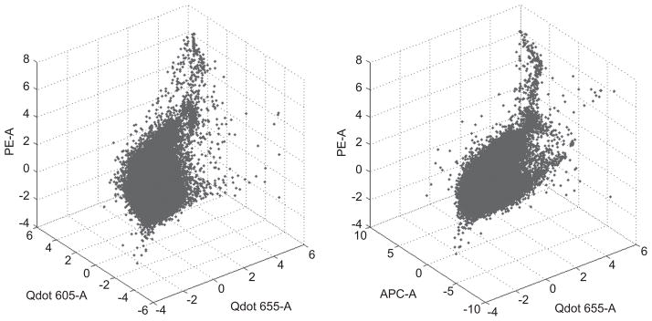
3D scatter plots of a randomly selected subset of the FCM data of Section 5.1 on 3 reporters. Left: Qdot 655-A vs. Qdot 605-A vs. PE-A. Right: Qdot 655-A vs. APC-A vs. PE-A.

Traditional mixture models have difficulties in identifying low probability component structure in fitting large datasets requiring many mixture components; the inherent masking issue makes it difficult to discover and quantify inferences on the biologically interesting but small clusters that deviate from the bulk of the data. We show this in the p = 10 dimensional example using standard dirichlet process (DP) mixtures (West et al., 1994; Escobar and West, 1995; Ishwaran and James, 2001; Chan et al., 2008; Manolopoulou et al., 2010). To fit the DP model, we used a truncated mixture with up to 160 Gaussian components, and the Bayesian expectation-maximization (EM) algorithm to find the highest posterior mode from multiple random starting points (L. Lin et al., submitted for publication; Suchard et al., 2010). The estimated mixture model with these plug-in parameters is shown in Figure 2. Many mixture components are concentrated in the main central region, with only a few components fitting the biologically important corner regions. To adequately estimate the low density corner regions would require a huge increase in the number of Gaussian components and an enormous computational search challenge, and is simply infeasible as a routine analysis.

Figure 2.

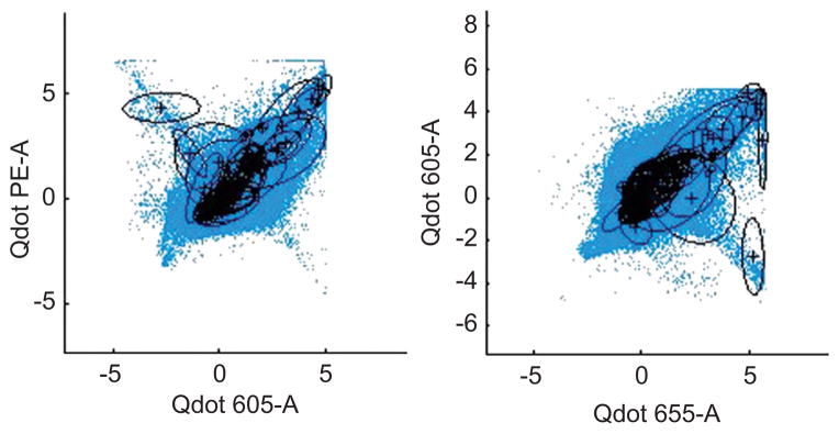
Data of Figure 1 on contours of 2-dimensional margins of fitted 10-dimensional DP Gaussian mixture.

3.2 Hierarchical model

We define a novel hierarchical mixture model specification that respects the phenotypic marker/reporter structure of the FCM data and integrates prior information reflecting the combinatorial encoding underlying the multimer reporters. Using f(·|·) as generic notation for any density function, the population density is described via the compositional specification

$$f\left({\chi }_{1:n}\mid \mathrm{\Theta }\right)=\prod _{i=1}^{n}f\left(b_i\mid \mathrm{\Theta }\right)f\left(t_i\mid b_i,\mathrm{\Theta }\right)$$ (1)

where Θ represents all relevant and needed parameters.

This naturally focuses on a hierarchical partition: (i) consider the distribution defined in the subspace of phenotypic markers first, to define understanding of substructure in the data reflecting differences in cell phenotype at that first level; then (ii) given cells localized – and differentiated at this first level – based on their phenotypic markers, understand subtypes within that now based on multimer binding that defines finer substructure among T-cell features.

3.3 Mixture model for phenotypic markers

Heterogeneity in phenotypic marker space is represented via a standard truncated Dirichlet process mixture model (Ishwaran and James, 2001; Chan et al., 2008; Manolopoulou et al., 2010; Suchard et al., 2010). A mixture model at this first level allows for first-stage subtyping of cells according to biological phenotypes defined by the phenotypic markers alone. That is,

$$f\left(b_i\mid \mathrm{\Theta }\right)=\sum _{j=1}^J{\pi }_{j}N\left(b_i\mid {\mu }_{b,j},{\mathrm{\sum }}_{b,j}\right)$$ (2)

where π_1:J are the component probabilities, summing to 1, and N(b_i|μ_{b, j}, Σ_{b, j}) is the density of the p_b–dimensional Gaussian distribution for b_i with mean vector μ_{b, j} and covariance matrix Σ_{b, j}. The parameters {π_1:J, μ_{b, 1:J}, Σ_{b, 1:J}} are elements of the overall parameter set Θ. Priors on these parameters are taken as standard; that for π_1:J is defined by the usual stick breaking representation inherent in the DP model, and we adopt proper, conditionally conjugate normal-inverse Wishart priors for the {μ_{b, j}, Σ_{b, j}}; see Appendix 7.1 for details and references.

The mixture model can be interpreted as arising from a clustering procedure depending on underlying latent indicators z_{b, i} for each observation b_i. That is, z_{b, i} = j indicates that phenotypic marker vector b_i was generated from mixture component j, or b_i|z_{b, i} = j~N(b_i|μ_{b, j}, Σ_{b, j}), and with P(z_{b, i} = j) = π_j. The mixture model also has the flexibility to represent non-Gaussian T-cell region densities by aggregating a subset of Gaussian densities. This latter point is key in understanding that Gaussian mixtures do not imply Gaussian forms for biological subtypes, and is used in routine FCM applications with traditional mixtures (Chan et al., 2008; Finak et al., 2009).

Bayesian analysis using Markov chain Monte Carlo (MCMC) methods augments the parameter space with the set of latent component indicators z_{b, i} and generates posterior samples of all model parameters together with these indicators. Over the course of the MCMC the z_{b, i} vary to reflect posterior uncertainties, while conditional on any set of their values the data set is conditionally clustered into J groups (some of which may, of course, be empty) reflecting a current set of distinct subpopulations; some of these may reflect one unique biological subtype, though realistically they generally reflect aggregates of subtypes that may then be further evaluated based on the multimer reporters. This is the key point that underlies the second component of the hierarchical mixture model, as follows.

3.4 Conditional mixture models for multimers

Reflecting the biological reality, we posit a mixture model for multimer reporters t_i, again utilizing a mixture of Gaussians for flexibility in representing essentially arbitrary non-Gaussian structure; we again note that clustering several Gaussian components together may overlay the analysis in identifying biologically functional subtypes of cells. We assume a mixture of at most K Gaussians, N(t_i|μ_{t, k}, Σ_{t, k}), for k = 1: K. The locations and shapes of these Gaussians reflects the localizations and local patterns of T-cell distributions in multiple regions of multimer. However, recognizing that the above development of a mixture for phenotypic markers has the inherent ability to subdivide T-cells into up to J subsets, we need to reflect that the relative abundance of cells differentiated by multimer reporters will vary across these phenotypic marker subsets. That is, the weights on the K normals for t_i will depend on the classification indicator z_{b, i} were they to be known. Since these indicators are part of the augmented model for the b_i we therefore condition on them to develop the model for t_i.

Specifically, we take the set of J mixtures, each with K components, given by

$$f\left(t_i\mid z_{b,i}=j,b_i,\mathrm{\Theta }\right)=\sum _{k=1}^K{\omega }_{j,k}N\left(t_i\mid {\mu }_{t,k},{\mathrm{\sum }}_{t,k}\right)$$

where the ω_{j, k} sum to 1 over k =1:K for each j. As discussed above, the component Gaussians are common across phenotypic marker subsets j, but the mixture weights ω_{j, k} vary and may be very different.

This leads to the natural theoretical development of the conditional density of multimer reporters given the phenotypic markers, defining the second components of each term in the likelihood function of equation (1). This is

$$\begin{array}{l}f\left(t_i\mid b_i,\mathrm{\Theta }\right)=\sum _{j=1}^{J}f\left(t_i,z_{b,i}=j\mid b_i,\mathrm{\Theta }\right)\\ =\sum _{j=1}^{J}P\left(z_{b,i}=j\mid b_i,\mathrm{\Theta }\right)f\left(t_i\mid z_{b,i}=j,b_i,\mathrm{\Theta }\right)\end{array}$$ (3)

$$\begin{array}{l}=\sum _{j=1}^J\left\{\frac{{\pi }_{j}N\left(b_i\mid {\mu }_{b,j},{\mathrm{\sum }}_{b,,j}\right)}{f\left(b_i\mid \mathrm{\Theta }\right)}\right\}\sum _{k=1}^K{\omega }_{j,k}N\left(t_i\mid {\mu }_{t,k},{\mathrm{\sum }}_{t,k}\right)\\ =\sum _{k=1}^K{\omega }_{i,k}\left(b_i\right)N\left(t_i\mid {\mu }_{t,k},{\mathrm{\sum }}_{t,k}\right)\end{array}$$ (4)

where

$${\omega }_{i,k}(b_i)=f{\left(b_i\mid \mathrm{\Theta }\right)}^{-1}\sum _{j=1}^J{\omega }_{j,k}{\pi }_{j}N\left(b_i\mid {\mu }_{b,j},{\mathrm{\sum }}_{b,j}\right).$$ (5)

Notice that the ω_{i, k}(b_i) are mixing weights for the K multimer components as reflected by equation (4); the model induces latent indicators z_{t, i} in the distribution over multimer reporter outcomes conditional on phenotypic marker outcomes, with P(z_{t, i} = j|b_i) = ω_{i, k}(b_i). These multimer classification probabilities are now explicitly linked to the phenotypic marker measurements and the affinity of the datum b_i for component j in phenotypic marker space.

From the viewpoint of the main applied focus on identifying cells according to subtypes defined by both phenotypic markers and multimers, key interest lies in posterior inferences on the subtype classification probabilities

$$P\left(z_{b,i}=c,z_{t,i}=c\mid {\chi }_i,\mathrm{\Theta }\right)\propto \sum _{(j,k)\in I_c}{\pi }_{j}N\left(b_i\mid {\mu }_{b,j},{\mathrm{\sum }}_{b,j}\right){\omega }_{i,k}\left(b_i\right)N\left(t_i\mid {\mu }_{t,k},{\mathrm{\sum }}_{t,k}\right),$$ (6)

for each subtype c =1:C, where I_c is the subtype index set containing indices of the Gaussian components that together define subtype c. Here

$$P(z_{b,i}=j,z_{t,i}=k\mid {\chi }_i,\mathrm{\Theta })\propto {\pi }_{j}N(b_i\mid {\mu }_{b,j},{\mathrm{\sum }}_{b,j}){\omega }_{i,k}(b_i)N(t_i\mid {\mu }_{t,k},{\mathrm{\sum }}_{t,k}),$$ (7)

for j =1:J, k =1:K, and the index sets I_c contains phenotypic marker and multimer component indices j and k, respectively. These classification subsets and probabilities will be repeatedly evaluated on each observation i =1:n at each iterate of the MCMC analysis, so building up the posterior profile of subtype classification.

One next aspect of model completion is specification of priors over the J sets of probabilities ω_{j, 1:K} and the component means and variance matrices {μ_{t, 1:K}, Σ_{t, 1:K}}. This is done using the structure of a standard hierarchical extension of the truncated DP model (Teh et al., 2006). Under a prior from this class, the ω_{1:J, 1:K} are naturally independent of the {μ_{t, 1:K}, Σ_{t, 1:K}}, and are also naturally linked across phenotypic marker components j; the specification of p(ω_{1:J, 1:K}) is detailed in Appendix 7.2.

We further take the Σ_{t, 1:K} as independent of the other parameters and with Σ_{t, k}~IW(Σ_t,k|δ_t, Φ_t) for some specified δ_t, Φ_t, corresponding to the usual conditionally conjugate prior.

The remaining aspect of the prior specification is that for μ_{t, 1:K}, the multimer model component location vectors, and it is here that the structure of the combinatorial encoding design comes into play.

3.5 Priors on multimer component location vectors

The levels of different multimers represented by subtype means μ_{t, 1:K} must be structured to reflect the combinatorial design. For any given epitope, reported fluorescent intensity levels are recognized as distributed around zero for cells lacking the corresponding cell surface receptor, in a range of low non-zero values, or at rather higher levels for cells targeted by the reporter. We capture this through a prior on the μ_{t, 1:K} linked to corresponding regions in reporter space, structured to also capture the prior knowledge implicit in the strategy of multimer combinatorial encoding.

Define anchor regions in the p_t–dimensional multimer reporter space by a set of R = 3^p_t anchor points, as follows. Represent by 0/L/H anchor points in any one multimer dimension, choosing specific values of L, H on the reporter scale. Set R = 3^p_t and define the set of R 3–vectors m_1:R via

$$m_r={(m_{1,r},m_{2,r},\dots ,m_{p_t,r})}^{\prime },r=1:R,$$

where m_{i, r} ∈ {0, L, H} and the m_r vectors represent all distinct R = 3^p_t combinations of 0, L, H for each of the p_t reporters. Effectively, the m_r identify all R subregions of the p_t – dimensional reporter space according to possible combinations of absent, low levels and high levels of each of the multimers being reported. For example, in the simplest case with p_t = 2, then R = 9, m_r vectors are the columns of the matrix

$$\left(\begin{array}{ccccccccc}0& 0& 0& L& L& L& H& H& H\\ 0& L& H& 0& L& H& 0& L& H\end{array}\right).$$

In some applications, this specification could be simplified to just two levels, e.g., by combining 0 and L levels. However, our data sets contain cell debris with light intensities at much lower levels compared to other cells in most dimensions, so the three levels are needed. In data sets that have been pre-cleaned of debris cells, a reduction to two levels could suffice, with appropriate modification of the following development.

Given the anchor vectors m_1:R, the prior for {μ_{t, 1:K}, Σ_{t, 1:K}} is now defined based on the following idea. We expect to see cell subtypes in a selection of the R regions linked to anchor points, and as earlier anticipate that distributions of reporters within subtypes may be heterogeneous. Hence any one subtype may be represented by a number of the μ_{t, k} that are clustered within one of the R regions, so that the resulting aggregate of the corresponding subset of the weighted N(t_i|μ_{t, k}, Σ_{t, k}) distributions reflects the reporter distribution for that cell subpopulation. This means a relevant prior for the μ_{t, k} will engender such clustering in the anchored regions reporter space while allowing for variability more globally. The natural model for this is to take the μ_{t, k} to be independent with marginal priors

$${\mu }_{t,k}~\sum _{r=1}^R{q}_{r}N\left({\mu }_{t,k}\mid m_r,Q_r\right)$$

for some variance matrices Q_r where, as a default, we take q_r = 1/R, for r = 1:R. In addition to allowing for the above described scientific clustering, this also allows for some or many of the R anchored regions to be “empty” in the sense that none of the μ_{t, k} are generated from the corresponding N(·|m_r, Q_r) component of this mixture prior.

Specification of the 3×3 variance matrices Q_r defines the expected levels of variation, and patterns of covariation, within a subset of the μ_{t, k} allocated to anchor region r. The default specification we make, following a broad study of the impact of variation in the values chosen is to base this on an overall scalar variance q and a set of specified pairwise correlations that relate to the anchor regions. For the latter, high abundance of two specific multimers – represented by H, H – is consistent with positive correlation in the corresponding elements of Q_r; low abundance of one and high abundance of the other – i.e., L, H – is consistent with negative correlation; lack of correlation is relevant when either one of the multimers is absent, i.e., 0, X for any X ∈ {0, L, H}. As an example when p_t = 3, for the 3 anchor regions r = s, u, v defined by m_s = (H, L, H)′, m_u = (0, L, L)′ and m_v = (0, 0, H)′, we take

$$Q_s=q\left(\begin{array}{ccc}1& {\rho }_n& {\rho }_p\\ {\rho }_n& 1& {\rho }_n\\ \rho & {\rho }_n& 1\end{array}\right),Q_u=q\left(\begin{array}{ccc}1& 0& 0\\ 0& 1& {\rho }_p\\ 0& {\rho }_p& 1\end{array}\right),Q_v=q\left(\begin{array}{ccc}1& 0& 0\\ 0& 1& 0\\ 0& 0& 1\end{array}\right),$$

respectively, where q controls overall levels of variation and ρ_p, ρ_n are specified positive and negative correlations. Following studies to evaluate specification, we take ρ_p = 0.6 and ρ_n = −0.6 as a default. The remaining Q_r matrices are filled out similarly corresponding to their anchor regions.

The specific anchor values of L, H are chosen to reflect known ranges of mean levels of low/high fluorescent intensities. This could be generalized to allow differing values that are specific to epitopes, and it is also possible to extend the Bayesian analysis to allow for uncertainty in these values by treating them as hyper-parameters. Standardized multimer measurements range from −4 to 10. Though the specific ranges differ somewhat across multimer, we take L = −4 and H = 6 for all multimers, defining prior ranges that allow for all experienced data regions. Similar comments apply to choice of values for the Q_r, in that the above specification might be relaxed by treating the ρ_p, ρ_n as hyper-parameters or even endowing each Q_r with, say, an inverse Wishart hyper-prior. Such extensions may be explored further in future in new applications. However, our current studies suggest that these extensions are overkill and unlikely to materially impact the resulting inferences; the specifications above have been customized to the known characteristics of FCM fluorescent reporter scales and we have evaluated a range of prior specifications and find strong levels of robustness to these specifications. The reasons for this are that the model already allows for uncertainty via the prior variability of the μ_{t, 1:K} around the means m_r, and overlays this with an ability to add multiple μ_{t, k} to any anchor region to fill-out a conditional mixture defining a flexible representation of the reporter distribution for the cell subtype in that region. That is, the model already has substantial degrees-of-freedom in adapting to observed data configurations.

3.6 Posterior computations

3.6.1 Augmented model and MCMC

Posterior computations use customized MCMC methods involving a combination of Gibbs sampling and Metropolis-Hastings. The overall strategy is standard in Bayesian computation, involving augmentation of the model parameter space by sets of mixture component indicators that (i) enable simulation of relevant conditional distributions for model parameters, and (ii) are themselves then imputed from relevant conditional posteriors as the MCMC proceeds. Thus we obtain posterior simulations for model parameters and mixture component indicators jointly, the latter feeding into follow-on inferences on subtype classification for each cell, among other things.

An outline to the augmentation ideas and the overall MCMC strategy is noted here, with full technical details given in Appendix 7.3. The full parameter set Θ is

$$\mathrm{\Theta }=\{({\mu }_{b,1:J},{\mathrm{\sum }}_{b,1:J},{\pi }_{1:J-1},{\alpha }_b),({\mu }_{t,1:K},{\mathrm{\sum }}_{t,1:K},{\omega }_{1:J,1:K},{\alpha }_t,\gamma )\}$$

where the first subset relates to the phenotypic marker mixture model and the second to that for the multimers. In the first, subset, α_b is a hyper-parameter underlying the DP prior for the phenotypic marker model whose role and prior are as defined in Appendix 7.1; similarly, the hyper-parameters α_t, γ_t of the multimer hierarchical DP model have roles and priors defined in Appendix 7.2.

The augmented model includes the phenotypic marker mixture component indicators z_{b, 1:n} earlier introduced as well as additional indicators underlying the hierarchical DP mixture for multimer mixture components conditional on the z_{b, 1:n}.

3.6.2 Post-MCMC analysis

MCMC fitting of mixture models suffer from the well-known label switching problem, complicating posterior inference. We address this using the state-of-the-art method for relabeling MCMC samples described and implemented in Cron and West (2011). At iterate s of the MCMC analysis with a current set of all model parameters Θ^(s) and sets of mixture component indicators generically denoted by Z^(s), this method relabels components in each of the mixtures: first for f(b_i|Θ) and then for f(t_i|b_i, θ). The computationally efficient and statistically effective relabeling strategy aims to match labels between MCMC iterates, so links the labels at iterate s with those at s−1, to best match the assignments of all n observations to labeled mixture components between the two steps. Our structured extension of mixture models requires a stagewise application of the strategy. Components of the phenotypic marker model ${\sum }_{j=1}^J{\pi }_{j}N\left(b_i\mid {\mu }_{b,j},{\mathrm{\sum }}_{b,j}\right)$ are relabeled first based on the phenotypic marker indicator matching; the relevant subset of the parameters are relabeled accordingly. Then, relabeling is applied to the multimer model ${\sum }_{k=1}^K{\omega }_{i,k}\left(b_i\right)N\left(t_i\mid {\mu }_{t,k},{\mathrm{\sum }}_{t,k}\right)$ with the consequent reording of the relevant parameters. Each of these is a straight application of the method of Cron and West (2011), and posterior inferences follow based on the sets of relabeled parameters.

Given the relabeled set of parameters for the hierarchical mixture model of equation (1), we follow previous work (Chan et al., 2008; Finak et al., 2009) in defining subtypes by aggregating proximate components π_jN(b_i|μ_{b, j}, Σ_{b, j}) ω_{i, k}(b_i)N(t_i|μ_{t, k,} Σ_{t, k}). That is, if a number of components cluster together and contribute to defining a mode in the mixture in one region of marker space, they are identified as a group and their renormalized average is taken as defining a subtype. This allows for a clear definition of subtypes, that may have quite non-Gaussian shapes, and is implemented by first identifying modes in the mixture of equation (1), and then associating each individual component with one mode based on proximity to the mode. An encompassing set of modes is first identified via numerical search; from some starting value x⁰, we perform iterative mode search using the BFGS quasi-Newton method for updating the approximation of the Hessian matrix, and the finite difference method in approximating gradient, to identify local modes. This is run in parallel from JK initial values ${\chi }^0={\left({\mu }_{b,j}^t,{\mu }_{t,k}^t\right)}^t$, j = 1:J, k = 1:K, and results in some number C ≤ JK unique modes. Grouping components into clusters defining subtypes is then done by associating each of the mixture components with the closest mode, i.e., identifying the components in the basin of attraction of each mode.

3.6.3 Computational implementation

The MCMC implementation is naturally computationally demanding, especially for larger data sets as in our FCM applications. Profiling our MCMC algorithm indicates that there are three main aspects that take up more than 99% of the overall computation time when dealing with moderate to large data sets as we have in FCM studies. These are: (i) Gaussian density evaluation for each observation against each mixture component as part of the computation needed to define conditional probabilities to resample component indicators; (ii) the actual resampling of all component indicators from the resulting sets of conditional multinomial distributions; and (iii) the matrix multiplications that are needed in each of the multivariate normal density evaluations. However, as we have previously shown in standard DP mixture models (Suchard et al., 2010), each of these problems is ideally suited to massively parallel processing on the CUDA/GPU architecture (graphics card processing units). In standard DP mixtures with hundreds of thousands to millions of observations and hundreds of mixture components, and with problems in dimensions comparable to those here, that reference demonstrated CUDA/GPU implementations providing speed-up of several hundred-fold as compared with single CPU implementations, and dramatically superior to multicore CPU analysis.

Our implementation exploits massive parallelization and GPU implementation. We take advantage of the Matlab programming/user interface, via Matlab scripts dealing with the non-computationally intensive parts of the MCMC analysis, while a Matlab/Mex/GPU library serves as a compute engine to handle the dominant computations in a massively parallel manner. The implementation of the library code includes storing persistent data structures in GPU global memory to reduce the overheads that would otherwise require significant time in transferring data between Matlab CPU memory and GPU global memory. In examples with dimensions comparable to those of the studies here, this library and our customized code delivers expected levels of speed-up; the MCMC computations are very demanding in practical contexts, but are accessible in GPU-enabled implementations. To give some insights using a data set with n = 500,000, p = 10, and a model with J = 100 and K = 160 clusters, a typical run time on a standard desktop CPU is around 35,000 s per 10 iterations. On a GPU enabled comparable machine with a GTX275 card (240 cores, 2G memory), this reduces to around 1250 s; with a more recent GTX680 card (1536 cores, 2G memory) this reduces further to about 520 s. The software will be available at the publication web site.

4 Simulation study

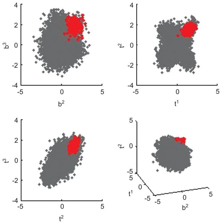
The simulation study conducted in the Section is to demonstrate the capability and usefulness of the conditional mixture model under the context of the combinatorial encoding data set. The simulation design mimics the characteristics of the combinatorial FCM context. Multiple other such simulations based on various parameters settings lead to very similar conclusions, so only one example is shown here. A sample of size 10,000 with p = 8 dimensions was drawn such that the first 5 dimensions was generated from a mixture of 7 normal distributions, such that, the last two normal distributions have approximate equal mean vectors (0, 5.5, 5.5, 0, 0)′, (0, 6, 6, 0, 0)′, and common diagonal covariance matrix 2I with component proportions 0.02 and 0.01. The remaining normal components have very different mean vectors and larger variances compared with the last two normal components. So b_i is the subvector of the first 5 dimensions, with p_b = 5. The last three dimensions are generated from a mixture of 10 normal distributions, where only two of them have high mean values across all three dimensions. The component proportions vary according to which normal component b_i was generated from. So t_i is the subvector of the last three dimensions, and p_t = 3. The data was designed to have a distinct mode such that all the five dimensions b², b³, t¹, t² and t³ are of positive values, the rest are negative. The cluster of interest with size 140 is indicated in red in Figure 3.

Figure 3.

Pairwise scatter plots and one 3-dimensional scatter plot of simulated data. The cluster of cells of interest is plotted in red. Here bⁱ is the ith dimension in the phenotypic marker subvector, and tⁱ is the ith dimension in the tetramer subvector. The lower right plot indicates that the cluster of interest is the outer layer of the sample under b², t¹ and t². The other 3 subplots show that the cluster is hard to identify with traditional 2-D gating.

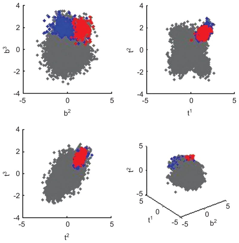
We first fit the sample with the standard DP Gaussian mixture model. Analysis allows up to 64 components using default, relatively vague priors, so encouraging smaller components. The Bayesian expectation-maximization algorithm was run repeatedly from many random starting points; the highest posterior mode identified 14 Gaussian components. Using parameters set at this mode leads to posterior classification probability matrix for the entire sample. The cluster representing the synthetic subtype of interest was completely masked as is shown in Figure 4.

Figure 4.

Scatter plots of synthetic data example as in Figure 3. Using standard DP mixture analysis, a relatively large subtype is identified. Cells assigned to this subtype are colored blue, and this blue region extends to include much of the actual subtype region, in red, in this synthetic data set. The analysis is unable to identify the correct subtype region.

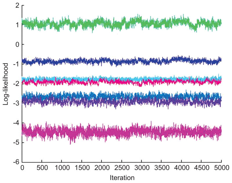
We contrast the above with results from analysis using the new hierarchical mixture model. Model specification uses J = 10 and K = 16 components in phenotypic marker and multimer model components, respectively. In the phenotypic marker model, priors favor smaller components: we take e_b = 50, f_b = 1, m = 0₅, δ_b = 26, Φ_b = 10I. Similarly, under multimer model, we chose e_t = 50, f_t = 1, δ_t = 24, Φ_t = 10I, L = −4, H = 6. We constructed m_1:R and Q_1:R for μ_{t, k} following Section 3.5, with q = 5, ρ_p = 0.6 and ρ_n = −0.6. The MCMC computations were initialized based on the specified prior distributions. Across multiple numerical experiments, we have found it useful to initialize the MCMC by using the Metropolis-Hastings proposal distributions as if they are exact conditional posteriors – i.e., by using the MCMC as described but, for a few hundred initial iterations, simply accepting all proposals. This has been found to be very beneficial in moving into the region of the posterior, and then running the full accept/reject MCMC thereafter. This analysis saved 20,000 MCMC draws for summary inferences. Global visuals addressing MCMC convergence, such as the trace plots of some log-likelihood components exemplified in Figure 5, are encouraging.

Figure 5.

Trace plot over the last 5000 MCMC iterates of computed values of the model of equation (1) on seven randomly selected data points.

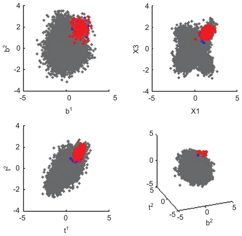
After relabeling and aggregating components based on the parameters at the last iterate this identified C = 29 modes in this “current” posterior sample. The posterior classification probabilities of equation (6) were computed for the last 3000 iterates, and data classification based on the resulting approximate posterior means. As shown in Figure 6, the hierarchical model analysis correctly identified 133 observations out of the 140 target sample.

Figure 6.

Scatter plots of synthetic data example as in Figures 3 and 4. The cluster of interest is plotted in red, and almost wholly overlays that identified by the hierarchical mixture model in blue.

5 Study of FCM data

5.1 Study of data from human blood samples

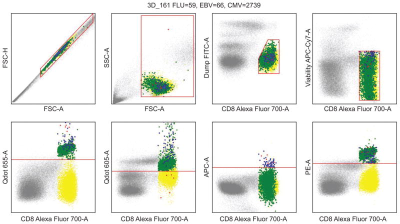
Peripheral blood samples were obtained from healthy volunteers for validation studies of the combinatorial encoding strategy. Peripheral blood mononuclear cells (PBMC) were labeled using the encoding strategy described; that is, with a mixture of fluorescent reporters indicating cell phenotype in phenotypic marker space and ability to recognize specific peptide-MHC epitopes in multimer space. The data set comprises n = 752,835 samples cells in p = 10 dimensions; the 10 measured features are the p_b = 6 phenotypic markers labeled FSC-A, FSC-H, SSC-A, Dump FITC-A, CD8 and Viability APC-Cy7-A, and the p_t = 4 multimers labeled Qdot 655-A, Qdot 605-A, APC-A and PE-A. The primary interest is to detect T-cells specific for CMV, EBV and influenza (Flu) virus peptides with the following combinatorial encoding scheme, where high intensities of the multimers in each define the T-cell subtype in reporter space:

$$\begin{array}{c}\text{CMV}=(\text{PE}-\mathrm{A},\text{Qdot}655-\mathrm{A},\text{Qdot}605-\mathrm{A}),\\ \text{EBV}=\text{PE}-\mathrm{A},\text{APC}-\mathrm{A},\text{Qdot}655-\mathrm{A}),\\ \text{FLU}=(\text{PE}-\mathrm{A},\text{Qdot}605-\mathrm{A},\text{APC}-\mathrm{A}).\end{array}$$

A subset of the data on some of the key features was already noted in Figure 1 in discussion of small probability structure of biologically interesting cell subtypes. Figure 7 illustrates the events determined to be positive for the targeted tetramer combinations for CMV, EBV and FLU using a standard manual gating procedure that is used as a reference plot for comparing with the model-based analysis here.

Figure 7.

Reference plot indicating clusters/subtypes of interest in the T-cell human blood data. A subset of the data is shown in gray, CD8+ T cells are plotted in yellow, CMV, EBV and FLU groups are plotted in green, red, and blue, respectively. These latter three identified subtypes contained 2739, 66 and 59 observations, respectively. Subtypes of interest are CD8+ and positive also in the three corresponding multimer features.

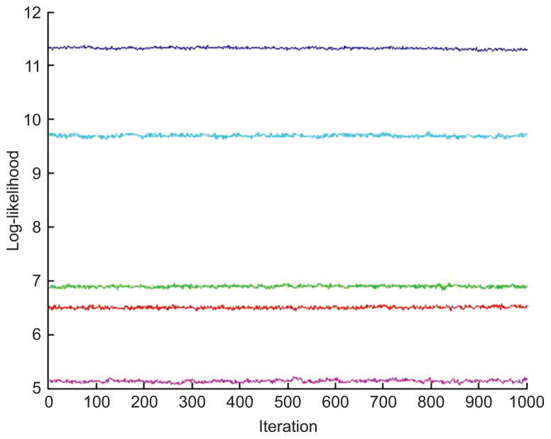
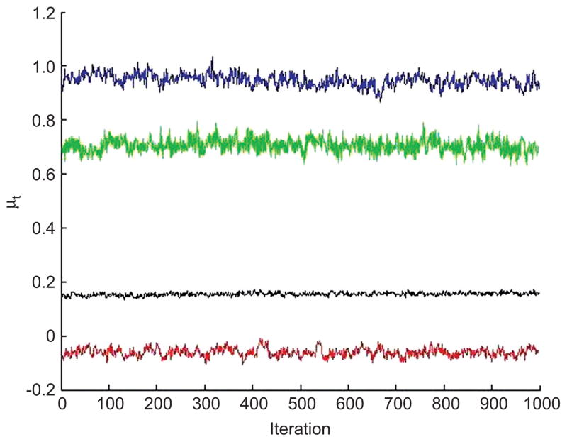
Model specification uses J = 100 and K = 100 components in the phenotypic marker and multimer model components, respectively. These are expected to be encompassing values with the model intrinsically able to cut-back to lower, data-relevant values based on the Bayesian DP mixture structure. In the phenotypic marker model component, priors favor larger numbers of smaller components: e_b = 50, f_b = 1, m = 0_pb×1, λ = 5, δ_b = p_b+1+10, Φ_b = 10I. Similarly, for the multimer model, e_t = 50, f_t = 1, δ_t = p_t+1+20, Φ_t = 10I, L = −4, and H = 6. We constructed m_1:R and Q_1:R for μ_t,k following Section 3.5 with q = 5, ρ_p = 0.6 and ρ_n = −0.6. The MCMC computations were initialized as detailed in the study of the synthetic data above and run for a total of 15,000 iterates. Posterior classification probabilities and individual parameters based the last 1000 iterate are used, again with exploration of visual diagnostics of convergence, e.g., Figures 8 and 9. While the overall MCMC certainly experiences mixing challenges, these convergence plots (and others, not shown) suggest we are at an acceptable phase of the MCMC for posterior inferences; longer and repeat runs support this.

Figure 8.

Trace plot over the last 1000 MCMC iterates of model density values on five randomly selected data points in analysis of human blood data.

Figure 9.

Trace plot over the last 1000 MCMC iterates of μ_t. Colors correspond to different randomly selected non-empty Gaussian components, with one dimension in μ_t selected for the trace plot.

The MCMC analysis outputs deliver the opportunity to enquire about a broad range of model characteristics; these include aspects of the mixture structure over phenotypic markers, while the primary biological focus rests on characteristics of the mixture structure over multimers and the classification of cells according to subtypes in multimer space. Some aspects of the former are worth noting initially. The fitted model indicates that there are approximately 1021 modes in the distribution. Contour plots of the estimated model in selected dimensions in Figure 10 show that a smaller number of Gaussian components can now represent the sample space much more effectively than with the original model as depicted in Figure 2.

Figure 10.

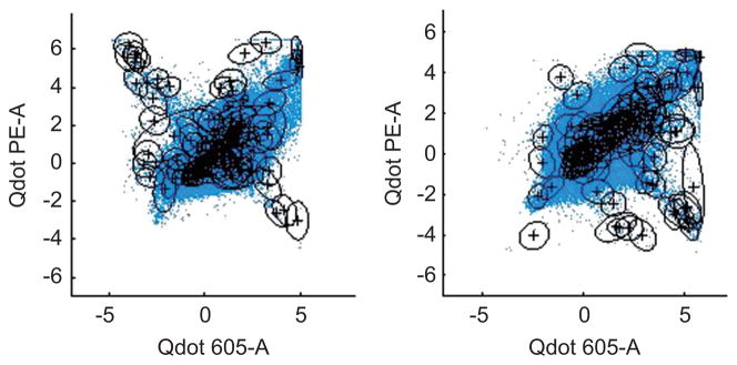
Scatter plots of the real data. The contours are the 2-dimensional margins on each Gaussian component in the full 10-dimensional mixture.

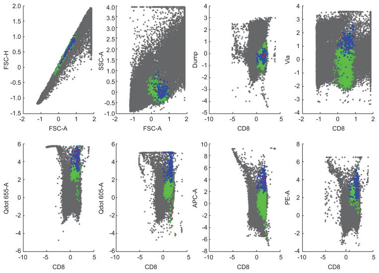
The MCMC analysis also delivers posterior samples of the z_b,i and z_t,i themselves; these are useful for exploring posterior inferences on the number of effective components out of the maximum (encompassing) value JK specified. Clusters that have high intensities for multimer combinations mapping to the multimer encodings are identified and shown in Figure 11. Our estimated CMV, EBV and FLU groups contains 12, 3 and 11 product of Gaussian components, respectively. The structured, hierarchical mixture model can flexibly capture many smaller Gaussian components as well as over-coming the masking issues of standard approaches. Some of the modes here have as few as 10 observations, reflecting the ability of the hierarchical approach to successfully identify quite rare events of potential interest.

Figure 11.

Identified clusters of interest. A subset of the data is shown in gray. CMV, EBV and FLU groups are plotted in green, red, and blue, respectively. The identified three groups contain 2849, 4 and 216 observations, respectively. The group with 4 events does not meet the cut-off of 10 events and 0.002% of CD8 for positive events we have suggested (Andersen et al., 2012) and may represent false positive or background events.

5.2 Study of data using classical single color FCM

We discuss aspects of one further example – a benchmark analysis on standard, single-color FCM data. Frelinger et al. (2010) used the truncated dirichlet process mixture model to analyze this standard data. As we discussed in Section 2, combinatorial encoding increases the ability to resolve subtypes. Suppose, for example, six “free” colors for peptide-MHC multimers. In the classical single-color approach, we could identify six different TCR specificities. In contrast, using a 3-color combinatorial approach, we could identify 20 different 3-color combinations and hence 20 different TCR specificities with a single blood sample. To identify 20 specificities with the classical approach would require testing four times as much blood from the same subject – clearly undesirable, and in many cases, impracticable.

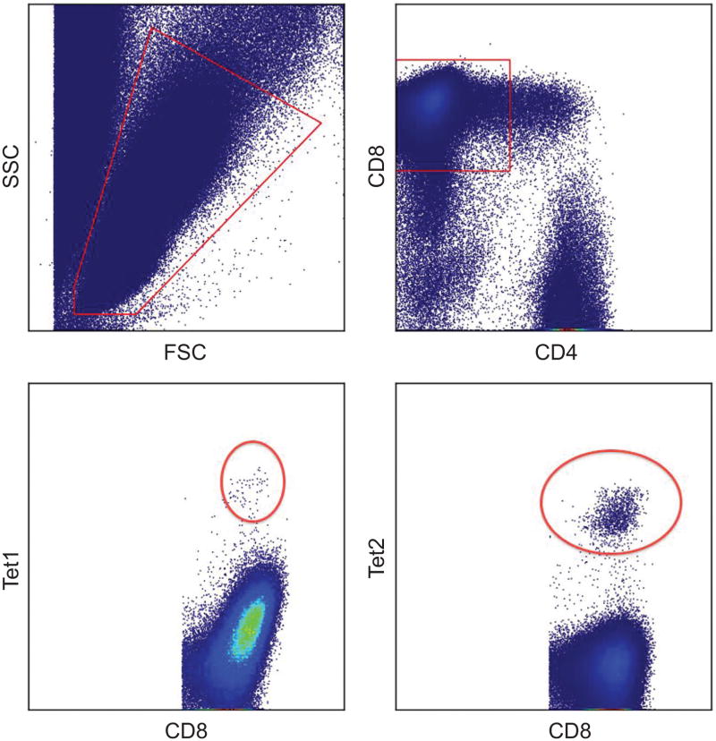
We apply our hierarchical model analysis to a classical data set to show its utility with single-color FCM, on top of its main aim and ability to resolve combinatorially encoded subtypes. The data comes from a subject with prostate cancer vaccinated with a set of tumor antigens (the data are post-vaccination) (Feyerabend et al., 2009); the sample size is n = 752,940. The assay has four phenotypic markers (FSC, SSC, CD4, CD8) and two multimers that report the prostate specific antigen PSA 141–150 FLTPKKLQCV, and the prostate specific membrane antigen PSMA 711–719 ALFDIESKV, respectively. The primary interest is to identify T-cells subtypes with high intensities of PSA and PSMA, respectively. Figure 12 illustrates the events determined to be positive for the PSA (labeled as tetramer 1, or Tet1 in the plot) and PSMA (Tet2) using a standard manual gating procedure; we use this simply as a reference plot for comparing with the model-based analysis here.

Figure 12.

Reference plot indicating clusters/subtypes of interest in the single-color encoded prostate cancer data.

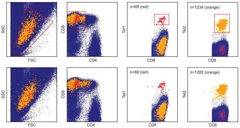
Model specification uses J = 100 and K = 100 components in the phenotypic marker and multimer models, respectively. The prior specifications and the MCMC computations were as detailed in Section 5.1. Following burn-in, posterior classification probabilities based on the last 1000 iterate are used. Based on thresholded probabilities, the two identified cell subtypes are shown in the bottom panel of Figure 13; these have cluster sizes of 68 and 1282, respectively, so represent extremely low probability subtypes. Comparing with the top panel of Figure 13, this demonstrates the ability of the hierarchical model to successfully identify cell clusters of interest in classical single-color data sets.

Figure 13.

Identified clusters of interest compared with manual analysis. The real data is shown in blue and the two clusters of interest are shown in red and orange, respectively. The top panel are the results from the manual gating, the bottom panel are the results from the hierarchical model.

6 Summary comments

We have defined and explored a novel class of structured, hierarchical mixture models with the applied goals of automated inference to identify specific cellular subtypes in very large samples of T-cells. The approach (i) involves a natural, model-based hierarchical partitioning of FCM phenotypic marker and multimer reporter measurements, and (ii) integrates a second stage hierarchical prior for the latter customized to the new biotechnological design of combinatorial encoding of multimers. The first step (i) represents key aspects of the biological reality: important cell subtypes defined by cell surface receptor function – as reported by the multimer data – are differentially represented across what is typically a large number of subtypes defined by phenotypic markers. Model-based stratification in phenotypic marker space effectively leads to sample dimension reduction that can overcome the inherent challenges of estimating what are typically low subtype probabilities. The second step (ii) addresses the specific features introduced in the recently proposed encoding method, a method that can greatly increase the number of T-cell antigen specificities distinguishable in limited biological samples using flow cytometry.

Combinatorial encoding can impact broadly on FCM studies by allowing a huge increase in the numbers of cell types detectable. This is particularly relevant in screening of optimal peptide epitopes in several areas, including vaccine design where the diversity of potential antigen-specific T cell subsets is substantial. Using conventional FCM methods with one fluorescent marker for each multimer-complex would require the collection and analysis of large (and infeasible) volumes of peripheral blood from each patient, and the sample sparing advantages of combinatorial encoding are key to a feasible screening strategy. Previous studies have shown the practicality of a dual encoding scheme (Hadrup et al., 2009; Newell et al., 2009; Hadrup and Schumacher, 2010; Andersen et al., 2012), and we are now able to appreciate the practical opportunities available with higher-order encoding.

We stress the key practical motivation lies in automated analysis and that this is critical in enabling access to the opportunity combinatorial methods open up. Standard visual gating is infeasible in higher-dimensional encoding schemes, and the broader FCM field is increasingly driving towards more relevant automated statistical approaches. Standard mixture models, however, lack the ability to identify the very small and subtle subtype structure of combinatorially encoded multimer events when applied to very large data sets; the masking by large background components can be profound. This is a key feature of the new model: as demonstrated in the examples: it is by design able to identify and quantify subpopulation structure related to relatively rare cell subtypes, i.e., to generate fitted models in which low probability mixture components are appropriately located in weakly populated regions of the p – dimensional sample space, and that are essentially undetectable using standard mixture approaches.

The hierarchical mixture model can in principle be customized for use in other FCM areas, such as in common laboratory studies using a “gating hierarchy” followed by “Boolean gating”. One example context uses first-stage phenotypic markers to home-in on smaller cell subsets characterized by functional cytokines, and this could be extended to use of the approach to distinguish combinations of different cytokines. We are considering some such developments in current research.

Part of the cost in application of the new, customized class of models is the implied computational burden; the structured MCMC is quite expensive in that respect. Efficient computational implementations are key, and we have developed coding strategies to maximally exploit the inherent opportunities for within MCMC parallelization customized to GPU processors. The code is optimized for CUDA/GPU processing with an accessible Matlab front-end (provided under an open source license) for implementing the model analysis as presented.

7 Appendix

7.1 Priors for parameters of phenotypic marker mixture

In the DP mixture model of Section 3.3, the traditional prior specification is as follows. Further background can be found in, for example Ishwaran and James (2001) or the summary appendix in Ji et al. (2009).

First, π₁ = ν₁, π_j = (1−ν₁)…(1−ν_j−1)ν_j, where ν_{j, j≠J}~Be(1, α_b),ν_J = 1, and the hyper-parameter α_b~Ga(e_b, f_b) for some specified e_b and f_b. Second, independently of the π_j the normal mean and variance matrices are independent across components with priors

$$({\mu }_{b,j},{\mathrm{\sum }}_{b,j})~N({\mu }_{b,j}\mid m,\lambda {\mathrm{\sum }}_{b,j})IW({\mathrm{\sum }}_{b,j}\mid {\delta }_b,{\mathrm{\Phi }}_b)$$

for some specified hyper-parameters m, λ, δ_b, Φ_b.

7.2 Priors for mixing weights in multimer mixtures

In the hierarchical DP mixture model of Section 3.4, the J sets of probabilities ω_j,1:K have priors defined from an underlying (truncated) hierarchical DP model as discussed in Teh et al. (2006). This extends the stick-breaking prior for mixture component weights to the set of J mixtures and links across them, with details as follows.

First, generate a K-vector of probabilities η_1:K via the stick-breaking construction

$${\eta }_k={\varphi }_k\prod _{l=1}^{k=1}\left(1-{\varphi }_l\right),k=1,\cdots ,K-1,$$

where ϕ_k~Beta(1, γ_t), k = 1, …, K−1 and ϕ_K = 1 and where γ_t~G(e_t, f_t) for some given hyper-parameters e_t, f_t.

Then, for each phenotypic marker component j = 1:J, generate the multimer mixture weights ω_j,1:K via

$${\omega }_{j,k}={\varphi }_{j,k}\prod _{l=1}^{k-1}\left(1-{\varphi }_{k,l}\right),k=1,\dots ,K-1,$$

where ${\varphi }_{j,k}~\mathit{Beta}\left({\alpha }_t{\eta }_k,{\alpha }_t\left(1-{\sum }_{l=1}^k{\eta }_l\right)\right)$, k =1, …, K−1, and ϕ_{j, K} = 1. We use hyper-priors α_t~G(a, c) for given hyper-parameters a, c.

7.3 MCMC analysis

Under the hierarchical mixture model specification, the MCMC analysis introduced in Section 3.6 has technical components as detailed here.

The use of an augmented model based on underlying, sample-specific, component indicator variables that induce the mixtures is, of course, key. We have already introduced the phenotypic marker mixture indicators z_b,i, latent indicators that underlie the assignment of each data point b_i to one of the j = 1:J components in the mixture of equation (2). At the second stage, we can apply the same strategy to the mixture for the t_i conditional on b_i of equation (4) by utilizing indicators z_{t, i}.

At each MCMC iterate, we resample subsets of Θ and the two sets of indicators Z = {z_b,i, z_t,i, i = 1:n} via the following sequence of sampling steps. In each conditional distribution the conditioning … represent the data and all other parameters and/or indicators; in some cases the need to be explicit about some of conditioning quantities is reflected in the use of the ^– superscript for their values at the preview MCMC iterate.

7.3.1 Update component indicator variables

For each i = 1:n in parallel due to conditional independence, update z_b,i and z_{t, i} by sampling from their conditional multinomial (number of trials = 1 in each case) posteriors defined by probabilities as follows:

$$\begin{array}{c}P(z_{b,i}=j\mid \dots )\propto {\pi }_{j}N(b_i\mid {\mu }_{b,j},{\mathrm{\sum }}_{b,j}),j=1:J;\\ P(z_{t,i}=k\mid \dots )\propto {\omega }_{i,k}(b_i)N(t_i\mid {\mu }_{t,k},{\mathrm{\sum }}_{t,k}),k=1:K.\end{array}$$

As z_b,i is conditionally independent of z_t,i, sampling the multimer model indicators is done in parallel with the phenotypic marker indicators.

7.3.2 Update phenotypic marker model parameters

7.3.2.1 Update phenotypic marker mixture weights and hyperparameter

Sampling mixture probabilities π_1:J and the hyperparameter of the DP model use a Metropolis-Hastings extension of the standard component distributions (Ishwaran and James, 2001; Ji et al., 2009), as follows. The mixture probabilities π_j are obtained from underlying beta variates ν_1:J−1 as detailed in Appendix 7.1. Hence new π_1:J samples are computed directly from resampled ν_1:J−1 samples. For the latter, we have

$$p\left(v_j\mid \dots \right)\propto Be\left(v_j\mid a_{b,j}+1,{\alpha }_b+\sum _{s=j+1}^J{a}_{b,s}\right)\prod _{k=1:K,i:z_{t,i}=k}{\omega }_{i,k}\left(b_i\right).$$

where $a_{b,j}={\sum }_{i=1}^N{1}_{z_{b,j=j}}$ for each j = 1:J−1. The complications here are that, since the π_j are functions of the ν_j, then ν_j is implicitly involved in both numerator and denominator terms of the product expression multiplying the base beta distributions. Hence we use a Metropolis-Hastings sampler for this step, based on a customized proposal distribution

$$v_j^{\ast }~Be\left(v_j\mid a_{b,j}+a_{u,j}+1,{\alpha }_b+\sum _{s=j+1}^J{a}_{b,s}+a_{u,s}\right)$$

with

$$\begin{array}{l}{a}_{u,s}=\sum _{i=1}^n{1}_{u_{t,i}=s},j=1:J-1\\ \left(u_{t,i}=s\right)=\underset{r=1:J}{max}{\pi }_{r}N\left(b_i\mid {\mu }_{b,r},{\mathrm{\sum }}_r\right){\omega }_{r,z_{b,i}}\end{array}$$

This proposal distribution is an approximation of p(ν_j|…) by taking off the denominator f(b_i|Θ)⁻¹ in the product expression and assuming that π_utiN(b_i|μ_uti Σ_uti)ω_utizb,i dominates the rest of the component values. Our experience with examples and the data analysis reported is that this generates acceptable convergence with acceptance rates for these components of the MCMC around 10–50%.

The weights π_1:J are then evaluated by the formula in Appendix 7.1. Next, the hyperparameter α_b is resampled from

$$\left({\alpha }_b\mid \dots \right)~Ga\left(J+e_b-1,f_b-\sum _{j=1}^{J-1}log\left(1-{\nu }_j\right)\right).$$

7.3.2.2 Update phenotypic marker component means and variance matrices

For each j = 1:J the mean μ_b,j has conditional posterior

$$p\left({\mu }_{b,j}\mid \dots \right)\propto N\left({\mu }_{b,j}\mid {\overline{\mu }}_b,{\overline{\mathrm{\sum }}}_b\right)\prod _{k=1:K,i:Z_{t,i}=k}{\omega }_{i,k}\left(b_i\right)$$

with

$${\overline{\mu }}_{b,j}=c_j\left(m/\lambda +\sum _{i:z_{b,i}=j}{b}_i\right)\text{and}{\overline{\mathrm{\sum }}}_b=c_j{\mathrm{\sum }}_{b,j}$$

where c_j = λ/(1+λa_1,j). Again we need a Metropolis-Hastings sampler for this step as the base normal distribution here is multiplied by a term that depends in complicated ways on μ_b,j. We use the customized proposal distribution ${\mu }_{b,j}^{\ast }~N\left({\mu }_{b,j}^{\ast }\mid {\overline{\mu }}_b^{\ast },{\overline{\mathrm{\sum }}}_b^{\ast }\right)$ where

$${\overline{\mu }}_{b,j}^{\ast }=c_j^{\ast }\left(m/\lambda +\sum _{i:z_{b,i}=j}{b}_i+\sum _{i:u_{t,i}=j}{b}_i\right)\text{and}{\overline{\mathrm{\sum }}}_b^{\ast }=c_j^{\ast }{\mathrm{\sum }}_{b,j}$$

with $c_j^{\ast }=\lambda /\left(1+\lambda a_{1,j}+\lambda a_{u,j}\right)$.

A similar structure and MCMC strategy arises for each of the j = 1:J variance matrices Σ_b,j; the conditional posteriors are

$$p\left({\sum }_{b,j}\mid \dots \right)\propto IW\left({\sum }_{b,j}\mid {\delta }_b+a_{b,j}+1,{\mathrm{\Phi }}_b+{\mathrm{\Psi }}_{b,j}\right)\prod _{k=1:K,i:z_{t,i}=k}{\omega }_{i,k}\left(b_i\right)$$

where

$${\mathrm{\Psi }}_{b,j}=\left({\mu }_{b,j}-m\right){\left({\mu }_{b,j}-m\right)}^{\prime }/\lambda +\sum _{i:z_{b,i}=j}\left(b_i-{\mu }_{b,j}\right){\left(b_i-{\mu }_{b,j}\right)}^{\prime }.$$

We use the customized proposal distribution

$${\mathrm{\sum }}_{b,j}^{\ast }~IW\left({\mathrm{\sum }}_{b,j}^{\ast }\mid {\delta }_b+a_{b,j}+a_{u,j}+1,{\mathrm{\Phi }}_b+{\mathrm{\Psi }}_{b,j}^{\ast }\right)$$

with

$${\mathrm{\Psi }}_{b,j^{\prime }}^{\ast }={\mathrm{\Psi }}_{b,j}+\sum _{i:u_{t,i}=j}\left(b_i-{\mu }_{b,j}\right){\left(b_i-{\mu }_{b,j}\right)}^{\prime }).$$

We update the pair (μ_b,j, Σ_b,j) together each iterate. We achieve acceptable convergence with acceptance rates for these components of the MCMC around 20–45%.

7.3.3 Update multimer model parameters

7.3.3.1 Update multimer mixture weights and hyperparameter

With the definitions and notation of the multimer mixture model parameters of Appendix 7.2, the logic and details of the MCMC steps are as follows.

For each k = 1:K ϕ_k has conditional posterior

$$p\left({\varphi }_k\mid \dots \right)\propto Be\left({\varphi }_k\mid 1,{\gamma }_t\right)\prod _{j=1:J,k=1:K}Be\left({\varphi }_{j,k}^{-}\mid {\alpha }_t{\eta }_k,{\alpha }_t\left(1-\sum _{l=1}^k{\eta }_l\right)\right).$$

To choose a proposal distribution, first, for each i = 1:n and independently over i, generate a set of auxiliary indicator variables q_i from conditional multinomials on k = 1:K cells with number of trials = 1 and

$$(q_i=k)\propto {\eta }_{k}N(t_i;{\mu }_{t,k},{\mathrm{\sum }}_{t,k}),k=1:K.$$

Given these sampled values, generate

$$\left({\varphi }_k^{\ast }\mid \dots \right)~Be\left(a_{q,k}+1,{\gamma }_t+\sum _{h=k+1}^K{a}_{q,h}\right),k=1:K-1,$$

where $a_{q,r}={\sum }_{i=1}^n{1}_{q_i=r}$ for each r = 1:K. We achieve acceptable convergence with acceptance rates for these components of the MCMC around 10–40%.

The sets of weights ω_j,k and the η_1:K probabilities are then evaluated by the formulæ given in Appendix 7.2. Further, the hyper-parameter γ_t is resampled from

$$\left({\gamma }_t\mid \dots \right)~Ga\left(K+e_t-1,f_t+\sum _{k=1}^{K-1}log\left(1-{\varphi }_k\right)\right).$$

Next, for each j = 1:J and k = 1:K, the latent probabilities ϕ_j,k of Appendix 7.2 have conditional posterior

$$p\left({\varphi }_{j,k}\mid \dots \right)\propto Be\left({\varphi }_{j,k}\mid {\alpha }_t{\eta }_k,{\alpha }_t\left(1-\sum _{l=1}^k{\eta }_l\right)\right)\prod _{k=1:K,i:z_{t,i}=k}{\omega }_{i,k}\left(b_i\right)$$

We use the customized proposal distribution

$$\left({\varphi }_{j,k}\mid \dots \right)~Be\left({\alpha }_t{\eta }_k+g_{j,k},{\alpha }_t\left(1-\sum _{h=1}^k{\eta }_h\right)+\sum _{h=k+1}^K{g}_{j,l}\right),$$

where $g_{j,k}={\sum }_{i=1}^n{1}_{z_{t,i}=k,u_{t,i}=j}$. We achieve acceptable convergence with acceptance rates for these components of the MCMC around 5–50%.

7.3.3.2 Update multimer component means and variance matrices

For each k = 1:K the mean μ_t,k is sampled using an additional auxiliary random quantity that allocates the multimer to one of the K anchor regions based on current parameters and indicators. That is, for each k independently, draw an auxiliary indicator τ_k from the multinomial with one trial and probabilities on k = 1:K given by

$$P\left({\tau }_k=r\mid {\mu }_{t,k}^{-},\dots \right)\propto q_{r}N({\mu }_{t,k}^{-}\mid m_r,Q_r),k=1:K.$$

Then draw (μ_t,k|C_k = r, …)~N (μ_{t, k}|m_t,k, M_t,k) where

$$m_{t,k}=M_{t,k}(Q_r^{-1}{m}_r+{\mathrm{\sum }}_{t,k}^{-1}\sum _{i:z_{t,i}=k}{t}_i)\text{and}{M}_{t,k}^{-1}=Q_r^{-1}+a_{t,k}{\mathrm{\sum }}_{t,k}^{-1}$$

with $a_{t,k}={\sum }_{i=1}^n{1}_{z_{t,i}=k}$.

Finally, resample the variance matrices from

$$\left({\mathrm{\sum }}_{t,k}\mid \dots \right)~IW\left({\mathrm{\sum }}_{t,k}\mid {\delta }_t+a_{t,k},{\mathrm{\Phi }}_t+\sum _{i:z_{t,i}=k}\left(t_i-{\mu }_{t,k}\right){\left(t_i-{\mu }_{t,k}\right)}^{\prime }\right)$$

References

- Andersen RS, Kvistborg P, Frøsig TM, Pedersen NW, Lyngaa R, Bakker AH, Shu Pthor Straten CJ, Schumacher TN, Hadrup SR. Parallel detection of antigen-specific t cell responses by combinatorial encoding of mhc multimers. Nature Protocols. 2012;7:891–902. doi: 10.1038/nprot.2012.037. [DOI] [PubMed] [Google Scholar]
- Chan C, Feng F, West M, Kepler TB. Statistical mixture modelling for cell subtype identification inflow cytometry. Cytometry A. 2008;73:693–701. doi: 10.1002/cyto.a.20583. [DOI] [PMC free article] [PubMed] [Google Scholar]
- Cron AJ, West M. Efficient classification-based relabeling in mixture models. Am Stat. 2011;65:16–20. doi: 10.1198/tast.2011.10170. [DOI] [PMC free article] [PubMed] [Google Scholar]
- Escobar MD, West M. Bayesian density estimation and inference using mixtures. J Am Stat Assoc. 1995;90:577–588. [Google Scholar]
- Feyerabend S, Stevanovic S, Gouttefangeas C, Wernet D, Hennenlotter J, Bedke J, Dietz K, Pascolo S, Kuczyk M, Rammensee HG, Stenzl A. Novel multi-peptide vaccination in hla-a2+ hormone sensitive patients with biochemical relapse of prostate cancer. Prostate. 2009;69:917–927. doi: 10.1002/pros.20941. [DOI] [PubMed] [Google Scholar]
- Finak G, Bashashati A, Brinkman R, Gottardo R. Merging mixture components for cell population identification in flow cytometry. Adv Bioinform. 2009:Article ID 247646. doi: 10.1155/2009/247646. [DOI] [PMC free article] [PubMed] [Google Scholar]
- Frelinger J, Ottinger J, Gouttefangeas C, Chan C. Modeling flow cytometry data for cancer vaccine immune monitoring. Cancer Immunol Immun. 2010;59:1435–1441. doi: 10.1007/s00262-010-0883-4. [DOI] [PMC free article] [PubMed] [Google Scholar]
- Hadrup SR, Bakker AH, Shu CJ, Andersen RS, van Veluw J, Hombrink P, Castermans E, thor Straten P, Blank C, Haanen JB, Heemskerk MH, Schumacher TN. Parallel detection of antigen-specific T-cell responses by multidimensional encoding of MHC multimers. Nat Methods. 2009;6:520–528. doi: 10.1038/nmeth.1345. [DOI] [PubMed] [Google Scholar]
- Hadrup SR, Schumacher TN. MHC-based detection of antigen-specific CD8+ T cell responses. Cancer Immunol Immun. 2010;59:1425–1433. doi: 10.1007/s00262-010-0824-2. [DOI] [PMC free article] [PubMed] [Google Scholar]
- Ishwaran H, James LF. Gibbs sampling methods for stick-breaking priors. J Am Stat Assoc. 2001;96:161–173. [Google Scholar]
- Ji C, Merl D, Kepler TB, West M. Spatial mixture modelling for unobserved point processes: application to immunofluorescence histology. Bayesian Analysis. 2009;4:297–316. doi: 10.1214/09-ba411. [DOI] [PMC free article] [PubMed] [Google Scholar]
- Lo K, Brinkman RR, Gottardo R. Automated gating of flow cytometry data via robust model-based clustering. Cytometry A. 2008;73:321–332. doi: 10.1002/cyto.a.20531. [DOI] [PubMed] [Google Scholar]
- Manolopoulou I, Chan C, West M. Selection sampling from large datasets for targeted inference in mixture modeling (with discusion) Bayesian Analysis. 2010;5:429–450. [PMC free article] [PubMed] [Google Scholar]
- Newell EW, Klein LO, Yu W, Davis MM. Simultaneous detection of many T-cell specificities using combinatorial tetramer staining. Nat Methods. 2009;6:497–499. doi: 10.1038/nmeth.1344. [DOI] [PMC free article] [PubMed] [Google Scholar]
- Pyne S, Hu X, Wang K, Rossin E, Lin T, Maier LM, Baecher-Allan C, McLachlan GJ, Tamayo P, Hafler DA, DeJager PL, Mesirov JP. Automated high-dimensional flow cytometric data analysis. Proc Natl Acad Sci. 2009;106:8519. doi: 10.1073/pnas.0903028106. [DOI] [PMC free article] [PubMed] [Google Scholar]
- Suchard MA, Wang Q, Chan C, Frelinger J, Cron AJ, West M. Understanding GPU programming for statistical computation: studies in massively parallel massive mixtures. J Comput Graph Stat. 2010;19:419–438. doi: 10.1198/jcgs.2010.10016. [DOI] [PMC free article] [PubMed] [Google Scholar]
- Teh YW, Jordan MI, Beal MJ, Blei DM. Hierarchical Dirichlet processes. J Am Stat Assoc. 2006;101:1566–1581. [Google Scholar]
- West M, Müller P, Escobar MD. Hierarchical priors and mixture models, with application in regression and density estimation. In: Smith AFM, Freeman PR, editors. Aspects of Uncertainty: A Tribute to D. V. Lindley. London: Wiley; 1994. pp. 363–386. [Google Scholar]