Mapping Argonaute and conventional RNA-binding protein interactions with RNA at single-nucleotide resolution using HITS-CLIP and CIMS analysis

Summary

Identifying sites where RNA binding proteins (RNABPs) interact with target RNAs opens the door to understanding the vast complexity of RNA regulation. UV-crosslinking and immunoprecipitation (CLIP) is a transformative technology in which RNAs purified from in vivo cross-linked RNA-protein complexes are sequenced to reveal footprints of RNABP:RNA contacts. CLIP combined with high throughput sequencing (HITS-CLIP) is a generalizable strategy to produce transcriptome-wide RNA binding maps with higher accuracy and resolution than standard RNA immunoprecipitation (RIP) profiling or purely computational approaches. Applying CLIP to Argonaute proteins has expanded the utility of this approach to mapping binding sites for microRNAs and other small regulatory RNAs. Finally, recent advances in data analysis take advantage of crosslinked-induced mutation sites (CIMS) to refine RNA-binding maps to single-nucleotide resolution. Once IP conditions are established, HITS-CLIP takes approximately eight days to prepare RNA for sequencing. Established pipelines for data analysis, including for CIMS, take 3-4 days.

Introduction

HITS-CLIP experiments provide the state-of-the-art means of identifying RNA binding sites for any RNABP of interest. The central feature of the protocol is the induction of covalent crosslinks between protein and a directly bound (within ∼ 1 Å) RNA by UV irradiation, which readily penetrates whole cells and even whole tissues. RNA-protein cross-linking is thus achieved without the addition of exogenous agents, such as photoactivatable reagents, or less selective chemical cross-linkers such as formaldehyde. In this way, endogenous protein-RNA interactions can be “frozen” in vivo for subsequent capture by immunopurification. After crosslinking, RNA is partially hydrolyzed to reduce bound RNA fragments to “footprint” sizes (typically ∼30-50nt) that can be cloned by RNA linker ligation and RT-PCR amplification. When these PCR products are sequenced on a high throughput platform, millions of unique RNA tags can be identified and mapped back to the genome, yielding unbiased transcriptome-wide RNA-protein binding maps.

Beyond the multitude of functions of conventional RNABPs in RNA regulation, the importance of miRNAs and related small regulatory RNAs in modulating gene expression is now firmly established. Mature, functional miRNAs are loaded in an obligate complex with Ago proteins, which are the catalytic components of the RNA-induced silencing complex (RISC) ^{1, 2}. When complexed with Ago, miRNAs bind complementary base-pairs in discrete mRNA target sites, primarily in 3′ untranslated regions (UTRs), leading to silencing by translation repression or nucleolytic turnover³. miRNA:mRNA base pairing occurs chiefly within a short ‘seed region’ spanning nucleotides (nts) 2-8 of the 21-22 nt miRNA. As little as 6 base pairs (bps) of complementarity is sufficient for functional miRNA targeting, so that the number of potential miRNA target sites in the transcriptome (∼1 in 4000 nt for a 6 nt seed) far exceeds the number of functional sites. For example, given a cell that expresses 400 miRNAs, a 4,000 nt mRNA would be expected to bind to some miRNA once every 10 nt, far exceeding the observed frequency of ∼2.3 Ago-miRNA binding sites/average transcript⁴. Indeed, although bioinformatic analyses have identified many miRNA targets, even the most rigorous efforts have had high rates of false positive and false negative prediction ^5-7. Ago HITS-CLIP provides an empirical means to identify functional miRNA target sites by mapping the global transcriptome occupancy of Ago:miRNA:mRNA ‘ternary’ complexes in vivo.

Ago HITS-CLIP requires minor modifications of the standard protocol to accommodate Ago's association with two distinct RNA species: miRNAs and target mRNAs. Here, size selection by SDS-PAGE following immunopurification is especially crucial, as Ago:miRNA complexes run at a lower molecular weight (∼110kD) than Ago:mRNA or Ago:miRNA:mRNA complexes (∼130kD and higher). Parallel isolation and analysis of these populations yields two datasets: a transcriptome-wide map of Ago binding footprints from the mRNA-enriched fraction (high MW) and an empirical catalog of functional, Ago-loaded miRNAs from the miRNA-enriched fraction (low MW). Interrogation of empirically determined Ago binding sites for miRNA seed sequences provides a rational framework for identification and validation of functional miRNA sites, with far lower false discovery rates than bioinformatic approaches alone⁴. Moreover, narrowing the sequence space of potential miRNA sites to bona fide Ago binding footprints facilitates the discovery of unconventional miRNA:mRNA pairing rules, such as the recent discovery that ∼15% of miR-124 sites in mouse brain possess a ‘G-bulge’ at position 5-6 that interrupts perfect complementarity⁸.

A final recent modification of HITS-CLIP analysis has capitalized on observations that reverse transcriptase is slightly error prone at the site of crosslinking^9-11. Crosslinking induced mutation sites (CIMS) can be used bioinformatically to map exact crosslinking sites, and hence RNA-protein interactions, with single nucleotide resolution ¹⁰.

Development of the protocol

CLIP grew out of two main frustrations with traditional approaches to studying RNA regulation in the course of studies of the neuron-specific RNA binding protein Nova. First were constraints on the ability to study RNA-protein interactions in an unbiased, genome-wide manner. Early efforts to define Nova RNA targets employed splicing-sensitive exon junction microarrays to probe RNA from the brains of wild-type and Nova-null mice. These studies demonstrated Nova-dependent splicing regulation of a biologically coherent set of pre and post-synaptic proteins^12,13. However, these results also highlighted a second difficulty, in that direct Nova targets could not be distinguished definitively from downstream or indirect effects of Nova loss-of-function. Although the presence of Nova's binding motif suggested that a substantial number of targets were direct¹⁴, the indirect nature of the study and the low complexity of Nova's binding motif (YCAY) prevented high-confidence conclusions.

The net result of these frustrations was an effort to develop a new means of genome-wide mapping of direct RNA-protein interaction sites, using UV crosslinking. UV crosslinking of proteins to nucleic acids had been used for some time in vitro (as reviewed¹⁵), where it was most commonly used to block reverse transcriptase and map sites of RNA-protein interaction¹⁶. The first CLIP experiments were aimed at identifying Nova-RNA interactions in viable brain tissue. The development of crosslinking conditions, RT conditions able to efficiently bypass sites of crosslinking, and RNA-linker ligation and sequencing protocols took our laboratory several years, and the first results were published with the sequences of ∼380 Nova-bound RNA tags in 2003 ¹⁷.

To extend CLIP to a truly genome-wide survey, two approaches were being considered—genome-wide tiling arrays and high throughput sequencing. Despite the high cost of the latter, it avoided noise and biases inherent in nucleic acid array hybridization, and this was the platform chosen for genome-wide CLIP or high-throughput sequencing CLIP (HITS-CLIP). The first HITS-CLIP results were obtained using the 454 Life Sciences platform by the end of 2006. It then took nearly two years to develop bioinformatic methods to parse the data both for information content and presentation for publication, finally resulting in the first HITS-CLIP paper in 2008¹⁸. Since then a flood of papers using HITS-CLIP has been published, opening the door to a new era in genome-wide analysis of RNA regulation in living cells—a systems biology approach to RNA regulation¹⁹.

These innovations led to the development of new kinds of maps. Principal among them were maps for Ago:miRNA:mRNA ternary complexes⁴, which offered the ability to deconvolute miRNA regulatory sites on a global scale. More recent is the advent of maps of RNABPs that play important roles in human disease. The latter have rapidly expanded beyond the paraneoplastic syndromes linked to Nova¹⁸ to cancer cells²⁰, motor neuron disease²¹ and intellectual disability²². For instance, the recently published RNA-binding map for Fragile-X Mental Retardation Protein (FMRP) led to the discovery of how it inhibits translation of specific neuronal mRNAs²².

Applications of the method

CLIP has proven to be a very robust protocol, with over 300 publications using the method since its initial publication. This includes analysis of RNA-protein interactions in a wide variety of organisms, including Eubacteria, fungi and yeast, C. elegans, and mouse and human tissues, along with many cell lines. Moreover, binding maps for a large variety of RNABPs with different nucleotide interaction motifs have been generated. For example, high quality maps have been generated for (and target motifs) Nova (YCAY)^17,18,23,24, PTBP1 and PTBP2 (CU-rich)^25,26, Elavl (AU and GU-rich)^27,28,29, TIA-1/TIAR (GU-rich)³⁰, TDP-43 (GU-rich)^21,31, hnRNP C (U-rich)³², RBFOX2 ([U]GCAUG)³³, MBNL2 (CUG) ³⁴, and others¹⁵.

HITS-CLIP has moved beyond the definition of “binary” RNA-protein maps, to generate “ternary” maps involving the Ago RNA binding proteins in complex with miRNAs and mRNAs. These more complex footprints have helped resolve miRNA binding sites on a genome-wide scale, and, importantly, have been repeated from their original description in mouse brain and HeLa cells⁴, to studies involving embryonic stem cells³⁵, T-cells³⁶, viral miRNAs³⁷, C. elegans³⁸, and HEK293T cells³⁹.

Comparison with other methods

RNA-IP (RIP) is a biochemically simpler protocol commonly that omits crosslinking. A prior review has contrasted these two in detail¹⁵. In brief, one main consideration is the higher rate of irrelevant RNAs (false positives) identified, and target RNAs missed (false negatives) with RIP relative to CLIP. The low stringency purification necessary to preserve RNA-protein interactions in the absence of crosslinking leads to false positive findings due to co-purifying RNAPBs. Moreover, the re-assortment of non-crosslinked protein-RNA complexes after cell lysis can produce both false positives and false negative findings⁴⁰. A second main consideration is that even where RIP is able to identify co-purifying transcripts, it can not pinpoint the sites of RNA-protein interaction, which is critical since sequence motifs of RNABPs are typically very short and degenerate.

Several CLIP variant protocols exist. The most divergent of these variations is PAR-CLIP, in which cells are fed 4-thiouridine (4-TU), a photoactivatable nucleoside analogue, prior to crosslinking³⁹. The motivation for this variation was that greater cross-linking could be achieved at comparable radiation doses, and that UV induced mutations (always U to C) marking the crosslink site at high frequency. These potential advantages have largely been obviated by the current HITS-CLIP and CIMS protocols discussed here, as recently shown in quantitative comparisons^10,41. High throughput sequencing is now so efficient that cross-linking efficiency is not a limiting factor. Single experiments with ∼100 mg of crosslinked brain tissue yield near saturating amounts of RNA tags for disparate RNABPs, including Nova¹⁸ and Ago⁴ (up to 5 × 10⁶ unique RNA tags per sample are now routine).

At the same time, the HITS-CLIP protocol described here avoids some drawbacks of PAR-CLIP, including the nucleotide bias introduced by the use of a single nucleoside analogue (4-TU) ⁴¹, cellular toxicity of 4-TU^42,43, and the inapplicability of PAR-CLIP to model organisms such as mice or to clinical or archived specimens.

Other CLIP variants more closely mirror the protocols described here. In CRAC-CLIP, affinity tagged proteins are used to purify RNA-protein complexes¹¹. CRAC-CLIP is largely interchangeable with the protocols presented here, with the important caveat that over-expression of epitope-tagged proteins may induce non-physiologic binding by altering RNA:protein stoichiometry. The other main variant, iCLIP, uses a modified strategy to clone crosslinked RNA tags that yields information about crosslinking sites, and in this respect is provides similar information to the CIMS analysis presented herein³². The distinguishing features of CLIP, CRAC-CLIP and iCLIP have been recently reviewed¹⁵.

Limitations

CLIP has proven robust and versatile in the analysis of many RNABPs in different biological contexts and a variety of organisms, ranging from eubacteria to human¹⁵, but some limitations bear noting. First are potential technical considerations, such as the availability of IP-competent antibodies. Whenever possible we strongly recommend the analysis of endogenous factors. The stoichiometry of RNA-protein complexes is a critical aspect of RNA regulation, and is likely to be perturbed when RNABPs or non-coding RNAs (e.g., miRNAs) are exogenously expressed⁴⁴. In addition, removal of RNABPs or miRNAs from a physiological context (e.g., enforced expression of a tissue-restricted factor in a cell line) will alter the repertoire of potential targets and undermine conclusions of biological consequence. When epitope tagging of RNABPs is warranted, efforts should be undertaken to minimize over-expression, for instance with tagging strategies that preserve endogenous expression or by titration of expression constructs to a minimal level.

A second set of caveats regards technical aspects of generating and cloning RNA tags. As described above, the method of RNA cleavage may bias the specific position of CLIP tags marking an RNABP ‘footprint’. A more substantial source of bias may be RNA linker ligation, because RNA ligase I has complex sequence and structural preferences that are only partially characterized^45,46. Technical modifications exist (e.g., RNA cleavage by alkaline hydrolysis) or are under development (e.g., ligation-independent cloning) that address these issues. Preliminary analyses of these modifications indicate that cleavage or ligation biases generally affect the 5′ and 3′ sites of RNA tags, but not the enumeration of binding sites as reflected by peak position or CIMS. However, these issues may have greater impact on RNABPs that bind to sequences that are refractory to cleavage or cloning, and so bear consideration.

A final potential limitation of the current HITS-CLIP protocol is the amount of material required to produce high-quality results. Necessary material will vary widely depending on the biological source and RNABP of interest; expression level, yield and purity of purification, cross-linking efficiency, and many other factors bear on this issue. For Ago HITS-CLIP we routinely retrieve high complexity data from moderate amounts of starting material (e.g., ∼1×10⁷ tissue culture or primary cells; ∼100mg mouse brain). More starting material, when not limiting, is helpful if purifications are scaled to preserve optimal signal-to-noise. Smaller amounts of starting material have been used successfully, especially for very abundant factors. We suspect that RNA linker ligation is the greatest ‘bottleneck’ during sample processing; an (optimistic) efficiency of ∼50% for 5′ and 3′ linker ligation entails a 75% loss of material, thus requiring more PCR amplification and reduced complexity. Ligation-independent cloning may remedy these constraints and permit analysis of minute cell populations (e.g., rare neuronal subtypes, sorted cells), but the protocol described here is subject to this limitation.

Experimental design

Provided here is a description of the major steps in the experimental protocol, including important controls at each stage (Fig. 1).

Figure 1. Overview of HITS-CLIP protocol.

A scheme for the experimental portion of the protocol is shown for Ago, with the miRNA drawn in blue and the mRNA in black. Phosphate (P) or hydroxyl (OH) status of RNA ends are indicated where pertinent to the protocol. (a) UV irradiation of live cells or tissue induces RNA-protein crosslinks (steps 1-3). (b) Material is lysed, RNA is partially digested, and the target protein is immunopurified with antibody coupled to magnetic beads (steps 4-17). (c) Alkaline phosphatase treatment removes 3′ hydroxyl to permit 3′ linker ligation (steps 18-20). (d) Radiolabeled (*), 3′ linker (red) is ligated to RNA tags (steps 21-22). Note that two options for radiolabeling are presented in the protocol. The figure depicts use of a radiolabeled 3′ linker, done for Ago and other cases where direct polynucleotide kinase (PNK) labeling gives high background. (e) Polynucleotide kinase treatment phosphorylates 5′ RNA ends, allowing subsequent 5′ linker ligation (steps 23-24). (f) Complexes are eluted from beads and separated by SDS-PAGE. Following transfer to nitrocellulose membrane, complexes are visualized by autoradiography (steps 25-32). (g) RNA is extracted from the desired membrane region by protease treatment, and 5′ linker (purple) is ligated to tags (steps 33-52). (h) Tags are amplified by RT-PCR (steps 53-77). (i) Following addition of sequencing adapters in a second PCR step, samples are sequenced on the Illumina Platform (steps 78-87).

Tissue crosslinking (steps 1-3)

UV crosslinking of cells and tissues is straightforward and the suitable dose for a given sample tolerates some margin of flexibility. The starting material affects somewhat the crosslinking procedure, because excess UV-irradiation can heat tissues and cause damage to RNA-protein complexes. Therefore, we typically apply less irradiation to tissue culture or primary cells in suspension or monolayer than to whole tissues such as brain. The original CLIP protocols irradiated freshly dissected tissue, either intact or triturated with a serological pipette. We have since observed excellent results by freezing samples in liquid nitrogen, grinding with a mortar/pestle, and keeping them frozen during UV-irradiation. Following irradiation, tissue can be frozen for long periods of time (years, in our experience). For initial experiments, a non-irradiated control sample is useful to assess PNK-mediated labeling in the absence of cross-linking. In most cases this control has little to no signal; however, there are some reported exceptions, including the tightly-bound ∼110kD Ago-miRNA complex, which is resistant to dissociation and therefore labeled even in the absence of cross-linking.

RNA digestion (steps 10, 11)

Reducing full-length RNA transcripts to ‘footprint’-sized fragments allows precise mapping of RNABP binding sites after sequence tag alignment. Most CLIP studies have used limited digestion with RNAse A, RNAse T1, micrococcal nuclease, RNAse I, or combinations thereof¹⁵. Experimental titration of RNAse is necessary to produce optimally sized RNA tags. The critical control here is an ‘over-digested’ sample, which should run near the predicted MW of the RNABP and provide a reference for the migration of partially digested experimental samples. In the case of Ago, two separate populations emerge at this stage: a ∼110kD Ago-miRNA band and a ∼130 kD Ago-miRNA-mRNA band. Another useful control is an ‘undigested’ sample, which indicates whether the input RNA is degraded.

Immunopurification of crosslinked RNABPs (steps 13-17)

This critical stage is likely to require the most troubleshooting and optimization, especially when prior immunopurification protocols do not exist for the antibody or RNABP of interest. It is beyond the scope of this protocol to teach IP technique, and the reader is referred to excellent manuals such as that by Harlow and Lane⁴⁷ and to a detailed discussion of these points in Green and Sambrook⁴⁸. Some general points to consider include:

• Antibody selection and optimization. In general, polyclonal antibodies have higher avidity than monoclonal antibodies, and may be amenable to harsher wash conditions and hence better protein purifications. However, it bears mentioning that we have encountered significant variability between lots for certain commercial polyclonals (e.g., Santa Cruz sc-10546, anti-Nova-2). Monoclonal antibodies offer the advantages of consistent performance and inexhaustible supply, but IP-competent monoclonals are unavailable for many proteins. Given the significant background that may be evident with some antibodies, whenever possible we also recommend repeating CLIP with two different antibodies and comparing the results. Such technical replicates combined with biologic replicates generate “gold-standard” HITS-CLIP datasets.

• IP/wash conditions. The most stringent IP/wash conditions that permit sufficient RNA recovery for sequencing will produce the “cleanest” results. As a minimum, we recommend comparing IPs with moderate stringency wash buffers (e.g., PXL, see below) and high stringency wash buffers (high salt, low salt, high detergent, etc.). We also recommend that once wash conditions have been established, investigators titrate the amount of antibody to an amount just below the point of fully clearing the RNABP from supernatants. This strategy will balance high recovery with minimized background due to excess antibody.

• Controls. Important controls for this stage include non-specific, isotype-matched antibody for monoclonals or species-matched sera for polyclonals. In addition, samples depleted of the RNABP of interest (e.g., siRNA-transfected cells or tissue from null mutant animals) can be very useful in proving the specificity of signal in experimental samples^17,22,30.

Labeling of RNA-protein complexes (steps 21-24)

In this protocol, RNA-protein complexes are visualized by polynucleotide kinase (PNK) radiolabeling. Direct labeling of RNA is most efficient and is suitable for most RNABPs examined. For Ago, direct PNK labeling produces high background signal and is inefficient for miRNAs, presumably because their 5′-end is buried in the protein interior⁴⁹. Therefore, the alternative strategy of radiolabeling the 3′ RNA linker was adopted during Ago HITS-CLIP development⁴. An inconvenience of this approach is lower labeling efficiency, although this affects only the autoradiogram exposure time, not the amount of retrievable RNA. Instructions for both direct PNK labeling and indirect ligation-mediated labeling are given in the Procedure. For new RNABPs, we recommend starting with direct labeling. If high background signal is a problem, ligation-mediated labeling may be advisable.

Size selection by SDS-PAGE (steps 25-36)

Size selection of labeled RNABP:RNA complexes by SDS-PAGE is critical for two reasons. First, this step visualizes the results of RNA digestion described above and thus allows isolation of RNA tags within an ideal size range. Second, SDS-PAGE separates the target RNABP from co-purifying contaminants, which may include other tightly associated RNABPs that survive the IP and washes or ones that cross-react with the antibody. For a number of RNABP/antibody pairs, including Ago, we observe contaminant bands on SDS-PAGE of unknown identity that might compromise results absent their removal at this stage.

RNA amplification (steps 38-87)

After purification and extraction, RNA tags must be amplified and modified with adapter sequences compatible with sequencing. In published studies and the protocol below, amplification is achieved by standard ligation of RNA linkers followed by RT-PCR. The first key concern at this step is avoidance of over-amplification, which will invariably favor predominance of certain PCR products and reduce sample complexity. We therefore go to significant lengths to preserve sample complexity by empirically determining an optimal PCR amplification range for each sample. In the procedure described below, RT products from each sample are divided across 8 PCR reactions. Four are run to different cycle numbers and analyzed by gel electrophoresis to determine an optimal cycle number. The remaining four are then run to the empirically determined cycle number and pooled for further processing. Other variations of this process are possible (as discussed previously⁴⁸). The attention paid to this point is at the discretion of the investigator, but in our hands even one unnecessary round of amplification can lead to a substantial drop in complexity (up to 2-fold per cycle). The second key concern at this step is avoidance of sample contamination. The most dangerous contaminants are adapter-bearing PCR products carried over from previous or parallel experiments. Such contaminants are highly stable on surfaces and in solutions, and their introduction at any point in the procedure can lead to false positive identification of RNABP binding sites during analysis. A second source of contamination is RNA from any source introduced into samples prior to adapter ligation, which will be carried through in subsequent amplification. In the following protocol, we describe strategies to avoid and identify contamination, including the use of linkers with short nucleotide ‘indexes’ to mark samples and flag cross-contamination.

Overview of bioinformatics analysis

The bioinformatics analysis of HITS-CLIP data bears some conceptual similarity to the analysis of ChIP-seq data, which capture DNA-protein interactions⁵⁰. However, HITS-CLIP data analysis has several distinct challenges due to technical issues (e.g., UV vs. formaldehyde crosslinking) and biological variables (e.g., RNA-protein interactions are convoluted with the wide dynamic range of RNA abundance).

Briefly, in the bioinformatic analysis of CLIP data, raw reads obtained from sequencers are first filtered to remove low-quality reads, and mapped back to the reference genome. Unambiguously mapped tags are then collapsed to remove potential PCR duplicates according to their genomic coordinates, and to identify unique CLIP tags that represent independent captures of protein-RNA interactions. Removal of PCR duplicates mitigates the bias introduced by preferential PCR amplification of particular sequence tags. However, this step could also exclude some genuinely unique CLIP tags that have the same coordinates by chance (i.e. individual molecules with the same 5′ and 3′ ends, a particular issue when sequence-specific RNases such as RNase A are used). These possibilities can be distinguished by including a degenerate barcode in the ligated RNA linker (before PCR amplification). Tags mapping to identical genomic coordinates, but ligated to linkers with different degenerate barcodes, are likely to represent unique binding events and thus retained. We have found that this strategy boosts the detection of unique tags by ∼20% (unpublished observations, C.Z.). Overlapping (or nearby, with relaxed stringency²⁵) unique CLIP tags are then clustered, and ranked by the ‘peak height’ of each cluster. Since the observed peak height is a function of both binding affinity and RNA abundance, there is still no straightforward way to infer quantitative binding affinity directly from CLIP data, in contrast to protein-DNA interaction analysis. Nevertheless, ranking of clusters by peak height reflects robustness of signals. Several methods have been proposed to evaluate the statistical significance of peak height above random backgrounds, although these methods differ in how gene expression level is normalized^4,25.

When CLIP experiments are performed with biological replicates, the data provide an opportunity to distinguish robust binding sites from those that are more transient or heterogeneous among individual samples. In addition to ranking clusters by peak height, we typically filter clusters by requiring ‘biological complexity’ (BC)--i.e. the presence of tags in all or a substantial fraction of biologically independent replicates ^{4,15,17,18,22}. Biological complexity reports on the presence or absence of tags in each replicate and does not take into account the exact number of CLIP tags in each experiment. A non-parametric meta analysis integrating these metrics was recently described, but is beyond the scope of the protocol here ^22,29.

CLIP tag cluster and peak analysis typically determines the RNABP footprints on RNA transcripts at a resolution of 30-60 nt. Recently we have exploited cross-linking induced mutation sites (CIMS) in HITS-CLIP datasets to map RNABP binding sites at single nucleotide resolution¹⁰. CIMS arise from the increased frequency (7∼22%, depending on specific RNABP) of reverse transcriptase errors at the exact nucleotide where amino acids crosslink to RNA, which was initially observed in a small set of Nova CLIP tags obtained by Sanger sequencing ⁹ and then in the interaction sites of several snoRNAs or ribosomal RNAs (rRNAs) with RNP proteins ^{51, 11, 52}.

To perform CIMS analysis, different types of mutations (i.e., nucleotide substitutions, deletions and insertions) are tracked. Analysis is restricted to mutations in unique tags, to avoid the complication of potential PCR duplicates. For a majority of RNABPs examined to date, UV crosslinking predominantly, if not exclusively, introduces nucleotide deletions, including Nova ¹⁰, Ago ¹⁰, Ptbp2²⁶, and Hu (unpublished observations, C.Z.) However, we and others also found other types of mutations induced by crosslinking. For example, both deletions and substitutions in Mbnl⁵³ and Lin28⁵⁴ HITS-CLIP data were identified (summarized in Table 1). In both cases, crosslinking induced substitutions appear more frequently than deletions, as judged from the number of robust CIMS and enrichment of motifs around CIMS. However, it bears noting that the identification of substitutions can be complicated by the existence of single nucleotide polymorphisms (SNPs), RNA editing sites, and other variables.

Table 1. Summary of RNABPs for which CIMS analysis has been performed following this protocol.

The frequency of deletions are reported as the percent of unique CLIP tags with one or more deletions. Since deletions introduced by mapping errors occur in general a much lower rate, these numbers represent a reasonable estimate of deletions introduced by crosslinking. For substitutions, whether they can be introduced by crosslinking is based on several criteria, including if they can provide appreciative improvement to pinpoint the motif. Because of the complication of substitutions caused by sequencing and other types of errors, it is difficult to give a quantitative estimate of the mutation rate caused by crosslinking. The base composition of the inferred crosslinked nucleotide is shown in the last column.

RNABP	Motif	Data source	Deletions (% tags)	Substitutions	Crosslinked nucleotide (left to right) A,C,G,U)
Nova	YCAY	50	Y (21)	N		Deletion
Ago	miRNA seed matches	4	Y (>8)	N		Deletion
Ptbp2	UCUY	23	Y (>7)	N		Deletion
Hu	U stretch	19	Y (21)	N		Deletion
Mbnl2	YGCY	31	Y (>9)	Y		Deletion
						Substitution
Lin28	AAGNNGAAGNG	45	Y (16)	Y		Deletion
						Substitution

CIMS have been identified in diverse sequence contexts in patterns consistent with established binding specificities. For example, Nova and Hu predominantly crosslink to U in the YCAY tetramer and U stretches, respectively. In contrast, Ptbp2 predominantly crosslinks to C of the UCUY motif, and Lin28 predominantly crosslink to G nucleotides. For Mbnl2, there also appears to be some difference in crosslink sites inferred from deletions and substitutions. Deletions occur in the last three nucleotides of the YGCY motif ³⁴; substitutions mostly occur in the third position C⁵³ (also unpublished analysis from C.Z. of the dataset from Charizanis et al. ³⁴). Since the exact nature and potential preferences of UV-induced protein-RNA cross-linking are not understood, we recommend that parallel analysis of all types of mutations be performed for new proteins.

For each type of mutations analyzed, CLIP tags are first clustered according to their genomic coordinates. Robust CIMS should be reproducibly supported by multiple CLIP tags, given sufficient sequencing depth. In contrast, mutations introduced by sequencing or alignment errors or other sources of noise should be randomly distributed. Therefore, statistical analysis can identify CIMS, which occur at a higher frequency than expected by chance. The two important parameters to measure robustness are the total number of tags overlapping each mutation site (k) and the number of tags with a particular type of mutations at the site (m). A permutation-based procedure can be used to evaluate if the observation of m tags with mutations at a specific position is statistically significant above the background, given k tags that overlap with the position in total. In permutation, each mutation is planted into a randomly selected CLIP tag, with the same offset relative to the 5′ end of the read as observed in the original tag. Therefore, this permutation preserves the distribution of CLIP tags in the transcriptome, as well as the positional bias of sequencing errors observed in the Illumina platform. An empirical false discovery rate (FDR) is assigned to each mutation site based on comparison of the two parameters k and m in real data and permuted data (see ref. ¹⁰ for more details).

To perform the tasks described here, a set of Perl scripts are used together with several standard unix system tools in command line in the step-by-step protocol. For some steps, similar tools might be publicly available, and can be used to replace the programs in this protocol (e.g., different sequence reads alignment programs, or c/c++ implementation of some of the steps to achieve faster speed). The focus of this computational protocol is to get a set of robust RNABP binding sites at a high resolution, starting from the raw data obtained from next-generation sequencing.

Downstream Analysis

Downstream analysis of HITS-CLIP data will depend on the goals of the investigator and the specific factor being studied. Although largely beyond the scope of this protocol, the Procedure includes steps to quantify binding peaks and to produce data tracks for visualization in UCSC Genome Browser ⁵⁵. The latter facilitates overlays with additional HITS-CLIP or other genome-wide datasets, such as RNA-seq expression data, conservation tracks, and predicted regulatory motifs such as miRNA seed sites.

Software

Software and documentation on installation and usage can be downloaded from http://zhanglab.c2b2.columbia.edu/index.php/CIMS. The software package is designed for linux or other unix-like operating systems, including Mac OS X. The software depends on several standard unix tools such as sort, awk, uniq, and cat, which are available in all common unix-like operation systems. Some scripts also require python, which is preinstalled in many linux releases and Mac OS X. If not, check http://www.python.org for more information. The program novoalign is used for read mapping; this software is available at http://www.novocraft.com. Basic familiarity with running command line tools is assumed in this protocol.

Materials

Caution: All experiments should be performed in accordance with relevant guidelines and regulations.

Reagents

Ultra-pure, nuclease and nucleic acid free water (e.g. Milli-Q)

1× Phosphate-Buffered Saline (PBS), RNAse-free (e.g., Invitrogen 10010-023)

Tween-20 (e.g., Sigma P9416)

Igepal/NP40 substitute (e.g., Sigma I8896)

sodium deoxycholate (e.g., Sigma D6750)

sodium dodecyl sulfate/SDS (e.g., Sigma L3771)

Tris pH 7.5, 1M stock solution (e.g., Sigma 252859)

EDTA, 0.5M stock solution (e.g., AM9261)

EGTA, 0.5M stock solution (e.g., BioWorld 40520008-2)

sodium chloride, 5M stock solution (e.g., Ambion AM9759)

potassium chloride, 2M stock solution (e.g., Ambion AM9640G)

magnesium chloride, 1M stock solution (e.g., Ambion AM9530G)

formamide (e.g., Sigma 47671-250ML-F)

ammonium acetate, 1M stock solution (e.g., Sigma A1542)

magnesium acetate, 1M stock solution (e.g., Sigma M5661)

Dynabeads, Protein A or Protein G-coupled (Invitrogen, 100-01D/100-03D)

Bridging antibody: rabbit anti-mouse IgG (only used for Ago CLIP; Jackson ImmunoResearch 315-005-008)

Antibody for immunoprecipitation (for Ago CLIP: mouse anti-Ago 2A8, Millipore MABE56)

RNase A (molecular biology grade; 20 units/mL) (e.g., Affymetrix/USB, 70194Y)

RQ1 DNAse (Promega, M6101)

RNasin Plus (Promega, N2611)

Alkaline Phosphatase (AP) (Roche, 10713023001)

T4 RNA ligase I, 10 units/μL (Fermentas, EL0021, supplied with BSA and 10× buffer)

10 mM ATP (e.g., Thermo Scientific #R0441, diluted 1:10 in water)

T4 polynucleotide kinase (PNK), 10 units/μL (NEB, M0201S)

[γ-³²P]ATP (3000 Ci/mmol) (Perkin Elmer, BLU002250UC)

Caution: All usage of radioisotopes should be done in strict accordance to the regulations and guidelines of one's institution. ³²P is a high energy beta emitter that poses an external dose hazard as well as potential internal dose hazards if ingested or inhaled. All steps should be conducted behind Plexiglas shielding of 3/8 inch thickness or greater. Materials should be stored in Plexiglas cases of this thickness. Waste disposal should follow institutional and governmental guidelines and regulations.

NuPAGE LDS sample buffer (4×) (Invitrogen, NP0008)

MOPS SDS running buffer (20×) (Invitrogen, NP0001)

Sample reducing agent (10×) (Invitrogen, NP0004)

Novex NuPage 8% Bis-Tris gels, with adapters (WG1002A)

Critical: Bis-Tris-buffered Novex NuPAGE gels run in MOPS or MES buffers are critical for CLIP, since it is buffered to maintain a neutral pH during electrophoresis. Standard SDS-PAGE gels (buffered by Tris) can rise up to pH ∼9.5, potentially leading to unwanted RNA hydrolysis. 8% gels, ideal for Ago, are only sold in the Midi size format. 10-12% gels, suitable for smaller RNABPs, are available in both Midi and Mini size format.

Nitrocellulose membrane (Protran BA-85, Whatman)

Critical: Pure, unsupported nitrocellulose facilitates extraction of RNA.

Bis-Tris transfer buffer (20×) (Invitrogen, NP0006)

Proteinase K, PCR grade (Roche, 03115828001)

Acid Phenol/Chloroform (Ambion, AM9720)

Caution: Phenol and its fumes are corrosive to skin, eyes, and airways. Phenol should be handled in a fume hood with suitable protective equipment, including eye protection, lab coat, and gloves.

NaOAc (3M stock; pH 5.2; molecular biology grade) (e.g., EMD Biosciences/Calbiochem, 567422)

Isopropanol (e.g., Fisher Scientific, AC327272500)

Ethanol (100% and 70% stocks) (e.g, Fisher Scientific BP2818-500)

GlycoBlue (Ambion, AM9516)

Superscript III, reverse transcriptase (Invitrogen, 18080044, supplied with DTT, 5× buffer, and dNTPs)

RT-PCR grade water (Ambion, AM9935)

Accuprime Pfx Supermix (Invitrogen, 12344-040)

Acrylamide:bisacrylamide (40% solution; 19:1) (Sigma A9926)

Caution: Monomeric acrylamide is a neurotoxin and should be handled with suitable protective equipment, including eye protection and gloves.

Ammonium persulfate (APS; 10% w/v; prepared fresh in water or stored as aliquots at −20°C) (Sigma A9164)

Tetramethylethylenediamine (TEMED) (Sigma T9281)

Urea (Sigma U54l8)

Vertical electrophoresis apparatus for polyacrylamide gels (e.g., Thermo Scientific, P8DS-2)

10 bp DNA ladder (Invitrogen, 10821-015)

Amplisize Molecular Ruler DNA ladder (Biorad 170-8200)

SYBR Gold (10,000× stock) (Invitrogen, S11494)

Caution: SYBR Gold is a DNA binding agent and thus potentially mutagenic. Suitable protective equipment, including eye protection, nitrile gloves, and lab coat should be worn when handling SYBR Gold.

Metaphor Agarose (Lonza, 50181)

Ethidium Bromide (Invitrogen 15585-011)

Caution: Ethidium bromide is a suspected mutagen. Suitable protective equipment, including eye protection, nitrile gloves, and lab coat should be worn when handling ethidium bromide.

Boric acid (Sigma B7901)

Reagent Setup

CRITICAL: Unless noted otherwise, the following buffers can be prepared in advance and stored for several months at 4° C. We prepare buffers using nuclease free salt and buffer stock solutions listed under Reagents above, bring to the desired final volume with Milli-Q water, and sterilize with a 0.22 μM filtration unit. Detergents (Tween-20, NP40/Igepal, sodium deoxycholate, and SDS) are prepared first as 10% stock solutions in Milli-Q water and diluted appropriately for buffer preparation. Scrupulous care should be taken to avoid contamination with nucleases or nucleic acids. Periodic replacement of reagents (every 3-4 months) is good practice to ensure reagent quality. If contamination is observed in later PCR amplification steps, these reagents should be discarded and re-prepared.

Bead Wash Buffer (BWB)

• 1× PBS (cell culture grade)

• 0.02% Tween-20 (v/v)

Lysis/immunoprecipitation buffer (1× PXL)

• 1× PBS (cell culture grade)

• 1% (v/v) Igepal/NP40 substitute

• 0.5% (w/v) sodium deoxycholate

• 0.1% (w/v) SDS

High stringency wash buffer

• 15 mM Tris-HCl, pH 7.5

• 5 mM EDTA, pH 8.0

• 2.5 mM EGTA, pH 8.0

• 1% (v/v) Igepal/NP40 substitute

• 1% (w/v) sodium deoxycholate

• 0.1% (w/v) SDS

• 120 mM NaCl

• 25 mM KCl

High salt wash buffer (compatible with anti-Ago 2A8; lower NaCl may be necessary for other antibodies)

• 1× PBS

• 1 M NaCl (final concentration, including the ∼140 mM NaCl present in PBS)

• 1% (v/v) Igepal/NP40 substitute

• 0.5% (w/v) sodium deoxycholate

• 0.1% (w/v) SDS

5× PXL buffer (used in Nova CLIP)

• 5× PBS

• 1% (v/v) Igepal/NP40 substitute

• 0.5% (w/v) sodium deoxycholate

• 1% (w/v) SDS

Low salt wash buffer (compatible with anti-Ago 2A8; other antibodies should be tested)

• 15 mM Tris-HCl pH 7.5

• 5mM EDTA

1× PNK buffer

• 50 mM Tris-HCl pH 7.5

• 10 mM MgCl₂

• 0.5% (v/v) Igepal/NP40 substitute

1× PNK + EGTA

• 50 mM Tris-HCl pH 7.5

• 20 mM EGTA

• 0.5% (v/v) Igepal/NP40 substitute

Proteinase K (PK) buffer

• 100 mM Tris-HCl pH 7.5

• 50 mM NaCl

• 10 mM EDTA

PK buffer + 7 M urea (prepared fresh each time; do not filter)

• 2.4g urea

• bring to 5ml with PK buffer and dissolve

5× Tris-Borate-EDTA (TBE) buffer (no filtration needed; stored at room temperature)

• 450 mM Tris-Borate, pH 8.3

• 10 mM EDTA

Formamide loading buffer (2×) (do not filter)

• 95% (v/v) formamide

• 10mM EDTA

Polyacrylamide Elution Buffer (stored at room temperature)

• 0.5 M ammonium acetate

• 10 mM magnesium acetate

• 1 mM EDTA

• 0.1% (w/v) SDS

RNA elution buffer (only needed for Box 2; stored at room temperature)

Box 2. Gel purification of RNA linkers (4 hours).

We generally purify RNA linkers by denaturing polyacrylamide electrophoresis after receipt from the manufacturer. It is important that only full-length RNA linkers are included in ligation reactions (i.e. steps 21 and 47) because the 5′ phosphate configuration and 3′-end blocking (with puromycin) ensure optimal efficiency. In addition, truncated linkers will complicate downstream bioinformatic analysis. Oligonucleotide manufacturers typically offer PAGE purification services, but in our hands the following protocol delivers far higher recovery.

1. Assemble a gel casting apparatus for a vertical electrophoresis system (e.g., Thermo Scientific Owl, P9DS-2 dual gel system) for a 1.5-mm-thick gel according the manufacturer's instructions.

2. For each gel, mix the following in a 50 ml conical tube:

   Component	Amt. per gel
   5× TBE	4 mL
   Urea	8.4g
   40% acrylamide:bisacrylamide (19:1)	5 mL
   Nuclease-free water	up to 20 mL

3. Immediately before pouring, add 200 μL of 10% APS and 7.5 μL of TEMED per gel. Cast gel and allow to polymerize at room temperature for 30 min.

4. Re-suspend RNA linker as supplied by manufacturer to 500 μM in RT-PCR grade water.

5. Add 50μL of 2× formamide loading buffer to 50μL RNA linker, mix, and load on 20% gel.

6. Run gel in 1× TBE at 350 V until bromophenol blue front is at bottom of gel.

7. Disassemble the gel apparatus and transfer the gel to plastic wrap on a screen (e.g., KODAK BioMax TranScreen LE) for UV shadowing.

8. RNA bands will appear dark against a fluorescent background. Carefully excise only the full-length RNA linker bands (it usually comprises that vast majority of product) and transfer gel slices to a RNAse-free 1.5ml microcentrifuge tube.

9. Crush gel slices using a 1mL syringe plunger.

10. Add 350μL RNA elution buffer to tube and incubate at 37° C in Thermomixer with shaking.

11. Transfer the gel slurry to a Nanosep spin filter and centrifuge according to manufacturer's instructions.

12. Transfer eluent to a 1.5 ml microcentrifuge tube. Precipitate linker by adding 1mL 100% ethanol and store at -20° C for 2 h to overnight.

13. Centrifuge sample at maximum speed in microcentrifuge for 20 min at 4° C.

14. Remove supernatant and wash pellet 1-2 times with 1mL 70% ethanol, spinning for 5 min each time.

15. Remove ethanol and dry pellet in SpeedVac or by air-drying.

16. Resuspend pellet in 50μL RT-PCR grade water.

17. Measure RNA concentration by UV absorbance. Dilute sample to 20μM with RT-PCR grade water, and dispense single-use aliquots to 1.5 mL microcentrifuge tubes. Store linkers at -80° C.

• 0.5 M ammonium acetate

• 10 mM magnesium acetate

• 1 mM EDTA

RNA linkers

• Puromycin-blocked 3′ linker (with a 5′ phosphate): RL3: 5′-P GUG UCA GUC ACU UCC AGC GG 3′-puromycin (Dharmacon; stored as a 20 μM, gel-purified and stored as described in Box 2). This is the standard 3′ RNA linker used for most RNABPs.

• Puromycin-blocked 3′ linker (lacking a 5′ phosphate): RL3(-P): 5′-OH GUG UCA GUC ACU UCC AGC GG 3′-puromycin (Dharmacon; stored as a 20 μM, gel-purified and stored as described in Box 2). This linker is required only if the 3′ linker will be radiolabeled according to the protocol in Box 1 (recommended for Ago CLIP).

• RL5 RNA linker (Dharmacon; 20 μM stock, gel-purified and stored as described in Box 2) 5′-OH AGG GAG GAC GAU GCG G 3′-OH

• RL5D RNA linker (Dharmacon; 20 <mu>M stock, gel-purified and stored as described in Box 2) RL5D: 5′-OH AGG GAG GAC GAU GCG Gr(N)r(N) r(N)r(N)G 3′-OH. This version contains a 4 nt degenerate sequence for identifying PCR duplicates.

Box 1. 5′ End Labeling of Dephosphorylated RL3 Linker (1 hour).

For some RNABPs, notably Ago, the signal:noise for imaging labeled RNABP:protein complexes is improved by ³²P-labeling the 3′ linker prior to ligation, rather than by directly labeling the RNA with PNK. This procedure will yield enough ³²P-labeled RL3 linker for 10 linker ligations reactions at step 21A(i). Note, this protocol is unnecessary when direct PNK labeling (steps 21B and 23B) is performed.

1. In an RNase-free 1.5ml microfuge tube, add in order:

   • 10.5μL RNAse-free water
   • 1μL RNasin Plus
   • 6μL RL3(-P) linker (20 μM) (IMPORTANT: 5′-end NOT phosphorylated)
   • 5μL 10× PNK buffer
   • 25μL [γ-³²P]ATP
   • 2.5μL T4 PNK enzyme

   Incubate at 37°C for 30 min.

2. Add 2 μL of 1 mM ATP, and incubate for an additional 5 min to fully phosphorylate the linker.

3. Prepare a mini-G-25 column. Resuspend the resin in the G-25 column by vortexing upside down, break off the bottom seal, and loosen the cap. Pre-centrifuge the column in a microcentrifuge tube in the microcentrifuge for 1 min at 735g, and transfer the G-25 column to a fresh, RNase-free microfuge tube.

4. Apply the phosphorylated linker sample to the resin, and spin the column for 2 min at 735g.

PAUSE POINT

The end-labeled linker can be used immediately or stored at −20°C until needed.

PCR primers

DP5 primer (from IDT; 20 μM stock prepared in TE buffer): 5′-AGG GAG GAC GAT GCG G-3′

DP3 primer (from IDT; 20 μM stock prepared in TE buffer): 5′-CCG CTG GAA GTG ACT GAC AC-3′

DSFP5 Solexa Fusion Primer (from IDT; 20 μM stock prepared in TE buffer):

5′-AATGATACGGCGACCACCGACTATGGATACTTAGTCAGGGAGGACGATGCGG- 3′

DSFP3 Solexa Fusion Primer (from IDT; 20 μM stock prepared in TE buffer):

5′-CAAGCAGAAGACGGCATACGACCGCTGGAAGTGACTGACAC- 3′

SSP1 Solexa Sequencing Primer (from IDT; 20 μM stock prepared in TE buffer):

5′-CTA TGG ATA CTT AGT CAG GGA GGA CGA TGC GG-3′

Equipment

Vacuum Driven Sterile Filtration Units (for buffer preparation) (e.g., Millipore SCGPU05RE)

1.5-ml Microfuge tubes (National Scientific Supply Co. SlickSeal tubes; RNase-free; cat. no. CN170S-GT, VWR#20172-945)

15-ml and 50-ml conical tubes (for harvesting of cells/tissue)

0.2-ml PCR tubes

Ultra-centrifuge tubes, polycarbonate (11 × 34 mm) (Beckman; cat. no. 343778)

Crushed ice in shallow trays of with a little water (that will fit in the UV crosslinker; used for tissue dissection and crosslinking)

Tissue culture dishes (35–150 mm; vessels for cross-linking)

Photographic film (Kodak MR, Fisher Scientific 05-728-24)

Plastic wrap

Glogos luminescent stickers (Agilent Technologies 420201)

Autoradiography cassette

Sterile scalpels

QIAquick Gel Extraction Kit (Qiagen 28704)

Quant-it DNA Assay Kit (high sensitivity) (Invitrogen, Q33120)

Cell-culture centrifuge (for 15- and 50-mL conical tubes; used to pellet cells)

Cold room

Freezer (−80°C) (for long-term storage of cell pellets)

Microcentrifuge (refrigerated)

UV-crosslinker (254 nm) (e.g., Stratalinker model 2400 [Stratagene] discontinued but widely available in molecular biology laboratories or Spectrolinker [Spectroline] with 254-nm bulbs)

Wheaton glass homogenizer (optional; see Step 5) (e.g. Thomas Scientific, 3432S90)

Ultracentrifuge, tabletop refrigerated (Beckman Optima MAX, TLA-120.2 rotor)

End-over-end mixer for microfuge tubes (to mix IPs)

Geiger counter or scintillation counter (see Step 20)

Magnetic bead collection apparatus (Invitrogen, 123-21D)

Temperature-adjustable dry block shaker (to keep Dynabeads from settling during incubations; Eppendorf Thermomixer R works well for this purpose)

Criterion Midi format Electrophoresis System (Biorad, 165-6001)

Note: Compatible with Novex Bis-Tris gels sold with adapters (see above)

Criterion Blotter (Biorad, 170-4070)

Vortex machine

PCR machine (such as the BioRad iCycler)

Vertical gel electrophoresis system (such as the Thermo Scientific Owl, P9DS-2 dual gel system)

UV Transilluminator (for visualizing SYBR Gold or ethidium bromide stained PCR products)

Horizontal electrophoresis system (such as the Thermo Scientific Owl B1A EasyCast mini gel system)

Access to high-throughput sequencing. CRITICAL This protocol is designed for Illumina sequencing platforms. In the future, other platforms will require different primers.

0.45 μm micro-centrifugal filter (e.g., Pall Life Sciences # ODM45C34)

Procedure

Sample preparation and UV Crosslinking (1-2 hours)

1 For adherent tissue culture cells, rinse once with PBS, and immerse with enough cold PBS to cover the monolayer. For suspension cells, pellet cultures by centrifugation and remove culture media. Re-suspend cells in 8 ml cold PBS and transfer to a clean 10 cm dish. For fresh tissue, triturate or dice to create gross suspension (small pieces of several mm³ are fine) in ice-cold PBS. Transfer tissue suspension to a 10 cm tissue culture dish and place on ice. For frozen tissue, grind in liquid nitrogen to a fine powder with a mortar and pestle and transfer to a petri dish on a bed of dry ice.

2 Irradiate tissue culture cells or powdered tissue once at 400 mJ/cm² and then again at 200 mJ/cm² in the UV crosslinker. Irradiate triturated tissue three times at 400 mJ/cm² in the UV crosslinker, swirling between each irradiation to keep it cold and maximize exposed surfaces for crosslinking. The Stratalinker or Spectrolinker crosslinkers have UV detectors that monitor actual dose delivered. The units are labeled such that 1=0.1 Joules/meter^2; hence a setting of 4000 on the machine is 400 mJ/cm².

3 Harvest the cells into a 15- or 50-ml conical tube and pellet by centrifugation at 1500 rpm at 4°C. Remove supernatant, re-suspend cell pellet in 1ml cold PBS, and transfer to a microfuge tube. Re-pellet cells (∼1000 × g for 5 min at 4°C in the microfuge), remove the supernatant, and freeze the packed cell pellets at −80°C until use (each tube should have a maximum of 200–300 μL of packed cells or tissue). Alternatively, monolayer cells can be released with EDTA or scraped directly into lysis buffer and the centrifugations omitted.

PAUSE POINT

Crosslinked tissue can be used directly for lysis and immunoprecipitation or flash frozen and stored at −80°C for months to years.

Bead Preparation (1 hour)

4 Pipet Dynabeads into a RNase-free 1.5-mL microfuge tube. Place tube in magnet, allow beads to collect on side of tube, and remove buffer. Wash beads three times in bead wash buffer (BWB) using 1 ml each time.

CRITICAL STEP

The volume of Dynabeads per sample should be adjusted for the amount of antibody used. We assume a capacity of ∼20 μg IgG per 100 μL Dynabeads. A minimum of 50 μL beads per sample is recommended to avoid loss during washes. The choice of protein A versus protein G conjugated beads depends on the species and/or isotype of antibody. Refer to the manufacturer's instructions for more details.

5 Resuspend the beads in BWB and add relevant antibody so that the final volume is the same as the original bead volume from step 4. If applicable, also prepare irrelevant antibodies controls, containing an equivalent amount of IgG as the anti-RNABP antibody.

CRITICAL STEP

As described in Experimental Design, the amount of antibody will be different for each antibody-RNABP combination (according to antibody avidity, RNABP abundance, etc.) and needs to be determined in pilot experiments. For most antibodies, we conjugate directly to magnetic beads. As an example, for Nova CLIP from one P13 mouse brain cortex, we use 24 μg of goat anti-Nova2 antibody (C-16, sc-10546) with 200 μL of protein G Dynabeads.

For Ago CLIP, we use the monoclonal antibody 2A8, which recognizes all four mammalian Ago proteins. We have found that 2A8 avidity is increased if it is coupled to DynaBeads via a ‘bridging antibody.’ For Ago CLIP from one P13 mouse brain cortex, we coat 200 μL of protein A Dynabeads with 50 μg of rabbit anti-mouse IgG _bridging_ antibody according to steps 4-7 below, wash away unbound bridging antibody with BWB, and then repeat steps 4-7 with 4 μL 2A8 anti-Ago ascites fluid. 2A8 and other anti-Ago antibodies are available from commercial sources (e.g., Millipore).

6 Rotate the tubes end-over-end at room temperature for 30 min (or up to overnight at 4°C).

7 Wash the loaded beads three times with 1× PXL, 1 mL per wash. For these and all subsequent washes, ensure that beads are fully resuspended. After the final wash, leave the beads in minimal volume of 1× PXL on ice until needed.

Lysis, RNAse digestion, and Immunoprecipitation (3-4 hours)

8 Resuspend the crosslinked tissue in each microfuge tube with 1× PXL and incubate on ice for 10 min. For crosslinked brain, suspend cell pellets in a volume of lysis buffer roughly 3× the volume of packed tissue. If the tissue is resistant to lysis, gentle mechanical disruption, for example with a Wheaton glass homogenizer, can be applied. For cell lysates from highly proliferative cultures, for example some immortalized cell lines, sonication can be used to reduce viscosity due to high DNA concentrations if necessary.

9 Add 30 μL of RQ1 DNase to each tube. Incubate at 37°C for 5 min at 1000 rpm in a Thermomixer.

10 Make a 1:100 dilution of RNase A in 1× PXL and make three further 10-fold serial dilutions (1,000; 1:10,000; and 1:100,000). As described in Experimental Design, testing a range of RNase concentrations is critical to determine a dose yielding optimally-sized RNA fragments, as assessed by autoradiography (see ‘Anticipated Results’). The overdigested sample (1:100 dilution of RNase A) is a critical control that will confirm crosslinking to protein of the appropriate molecular weight.

CRITICAL STEP

Optimal RNAse concentrations vary significantly for different RNABPs and input materials. The concentration of lysate (i.e. mass of material per volume lysis buffer) also dramatically affects the rate of RNAse digestion. Do not assume that RNAse titrations performed in one source material (e.g., cell line or tissue) are valid for another, even for the same protein. The RNAse dilution range specified above is deliberately broad; finer titration in future experiments can maximize the yield of appropriately sized RNA tags (see ‘Anticipated Results’ and Fig. 2a).

Figure 2. Sample CLIP autoradiograms (step 34).

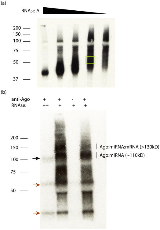
(a) An autoradiogram is shown for CLIP of the RBP TIA1 purified from human CD4+ T-cells. A RNAse titration was performed, which shows the overdigested complex in the leftmost lane running as a single band near the predicted MW (∼42 kD), and a smear extending upwards for progressively lower RNAse concentrations. The yellow box indicates an appropriate region to cut out for RNA extraction. (b) An autoradiogram is shown for CLIP of Ago from human T-cells, using the monoclonal 2A8 pan-Ago antibody. The first lane is an overdigested control, showing the ∼110kD band (black arrow). At lower RNAse concentrations (lanes 2 and 4), two populations are visible: the ∼110 kD Ago:miRNA complex, and the >130 kD Ago:miRNA:mRNA complex. Lane 3 is a control mouse IgG, showing the dependence of signal on 2A8. Note that contaminant bands (red arrows) are present in 2A8 IPs; the SDS-PAGE size selection is critical to diagnose and remove these contaminants.

11 For each RNAse concentration to be tested, add 10 μL diluted RNase per 1 ml of crosslinked lysate. Incubate at 37°C for 5 min and transfer to ice. Following this step lysates should be kept ice-cold to minimize further RNAse digestion. An RNAse inhibitor (e.g., RNAsin Plus at 0.2U to 1U per μL) can also be added to the lysates to quench RNase activity.

Save an aliquot of the lysate (∼10 μL) for subsequent immunoblot analysis (to confirm that your RNABP is not pelleted by the 32,000g clarification centrifugation below).

12 Centrifuge the lysates in a pre-chilled tabletop ultracentrifuge (in 11×34mm polycarbonate tubes in a TLA120.2 rotor) at 32,000g (RCF_avg; e.g., 30,000 rpm in the TLA120.2 rotor) for 20 min at 4°C. This step can lead to a ‘cleaner’ IP for many proteins, particularly from tissue lysates, but it must be confirmed that the protein of interest is not lost in the pellet.

Save 10–20 μL as both a post-centrifugation aliquot and a sample of the input to the IP for immunoblot analysis.

13 Transfer the supernatant to the tube containing antibody-bound beads from Step 7.

14 Rotate the beads/lysate mix end-over-end for 1-2 h at 4°C.

15 Remove the supernatant and save 10–20 μL of the _post-IP_ aliquot for immunoblot analysis to confirm depletion of target antigen from the lysate.

16 Wash the beads with cold wash buffers. As described in Experimental Design, pilot experiments should be done to determine the maximum stringency tolerated for post-IP washes, testing high-salt, low-salt, and high stringency (i.e. high ionic detergent) wash buffers. For Ago with 2A8 antibody, a standard wash protocol includes 2-3 washes with 1× PXL followed by 1-2 washes each with high-salt, high-stringency, and low-salt (see Reagent Setup). The wash protocol used for Nova consists of 3 times 1× PXL washes and 1 time 5× PXL wash buffer.

17 Wash beads twice with 1× PNK buffer.

PAUSE POINT

Cross-linked RNA-protein complexes are stable and can be left on washed beads in T4 PNK buffer overnight. Longer storage is not recommended, as there is risk of gradual dissociation of protein-antibody complexes (depending on the avidity of the antibody in use).

Dephosphorylation of RNA tags (1 hour)

18 Flash spin beads and remove residual PNK buffer. Resuspend beads in dephosphorylation master mix, prepared as follows, thoroughly by gentle vortexing. A total reaction volume of 80 μL should be used for no more than 400 μL of Dynabeads, starting volume. Here and for all subsequent enzymatic steps, volumes can be scaled down for smaller bead volumes to a minimum volume of 40 μL.

In an RNase-free 1.5-mL microfuge tube, prepare (per sample):

RNase-free water	67 μL
Dephosphorylation buffer, 10×	8 μL
Alkaline phosphatase	3 μL
Optional: RNAsin Plus (Promega).	2 μL

19 Incubate the reaction in a Thermomixer R at 37°C for 20 min, shaking at 1000 rpm for 15 sec every 2 min.

20 Wash the beads once with 1 mL of 1× PNK Buffer, once with 1 mL of 1× PNK+EGTA buffer, and twice with 1 mL 1× PNK buffer. Leave beads on ice in small volume of 1× PNK buffer until ready for the next step.

3′ RNA Adapter Ligation, On-Bead (overnight)

21 Prepare a 3′-linker ligation master mix. Use option A for Ago (ligation of ³²P-labeled RL3 linker) or option B for Nova and most other RNABPs (ligation of unlabeled RL3 linker).

A. For Ago: Ligation of ³²P-labeled RL3 linker

1. Prepare a 3′-linker ligation master mix with the following components for each tube:

   RNase-free water	47 μL
   T4 RNA Ligase Buffer, 10×	8 μL
   BSA (1mg/mL)	8 μL
   10 mM ATP	8 μL
   32P-labeled RL3 linker (prepared as in Box 1)	5 μL
   T4 RNA Ligase I	2 μL
   Optional: RNAsin Plus (Promega).	2 μL

2. Flash spin beads and remove residual buffer, then resuspend thoroughly in 80 μL 3′-linker ligation mix by gentle vortexing. Keep on ice while setting up the reaction, then incubate the bead mixture at 16°C overnight in a Thermomixer R, shaking at 1000 rpm for 15 sec every 2 min.

B. For Nova and most other RNABPs: Ligation of unlabeled RL3 linker

1. Prepare a 3′-linker ligation master mix with the follow components for each tube:

   RNase-free water	44 μL
   T4 RNA Ligase Buffer, 10×	8 μL
   BSA (0.2 mg/mL)	8 μL
   10 mM ATP	8 μL
   RL3 linker (IMPORTANT: with 5′-phosphate) @ 20 μM	8 μL
   T4 RNA Ligase I (Fermentas)	2 μL
   Optional: RNAsin Plus (Promega).	2 μL

2. Perform Step 21A(ii).

22 Wash the beads one time with 1× PNK buffer, one time with high-salt wash buffer, and two times with 1× PNK buffer. Leave beads on ice in small volume of 1× PNK buffer until ready for the next step.

5′ phosphorylation of RNA tags (1 hour)

23 Prepare a 5′ phosphorylation mix. Use option A if step 21A was followed above, or option B if 21B was followed.

A. If step 21A was followed above: phosphorylation with cold ATP

1. Prepare a 5′ phosphorylation mix with the following components per tube:

   RNase-free water	60 μL
   T4 PNK Buffer, 10×	8 μL
   10 mM ATP	8 μL
   T4 Polynucleotide Kinase	4 μL

2. Resuspend beads thoroughly in 80 μL phosphorylation mix, and incubate in a Thermomixer R at 37°C 20 min, shaking at 1000 rpm for 15 sec every 2 min.

B. If step 21B was followed above: radiolabeling with ³²P-γ-ATP

1. Prepare a 5′ phosphorylation mix with the following components per tube:

   RNase-free water	66 μL
   T4 PNK Buffer, 10×	8 μL
   T4 Polynucleotide Kinase (NEB)	4 μL
   32P-γ-ATP (3000 Ci/mmol)	1-2 μL

2. Resuspend beads thoroughly in 80 μL phosphorylation mix, and incubate in a Thermomixer R at 37°C 20 min, shaking at 1000 rpm for 15 sec every 2 min.

3. Important: Add 1 μL of cold 10mM ATP to each tube and incubate for an additional 5 min in a Thermomixer R at 37°C, shaking at 1000 rpm for 15 sec every 2 min. This ‘cold chase’ is critical to ensure complete phosphorylation of RNA tags (and hence efficient 5′ linker ligation), since the total concentration of ATP in ³²P-γ-ATP preparations is very low.

24 Wash the beads three times with 1 mL of 1× PNK+EGTA buffer. Leave beads on ice in small volume of buffer until ready for the next step.

Caution

All washes will contain radioactive material that must be discarded appropriately.

RNABP:RNA Complex Purification by SDS-PAGE and Membrane Transfer (3-6 hours)

25 Flash spin beads and remove residual buffer. Resuspend beads in 1× LDS sample loading buffer prepared as follows (per lane of gel):

• 7.5 μL LDS sample buffer

• 22.5 μL 1× PNK/EGTA buffer

• Optional (see below): 3 μL Sample Reducing Buffer (Invitrogen) or 0.5M DTT

CRITICAL STEP

Adjust resuspension volume based on how many gel lanes each sample will be divided across. Overloading gel lanes can result in distorted migration of samples due to excessive IgG from IP antibody; a maximum of ∼20 μg IgG should be loaded in each lane. Similarly, the decision of whether to add reducing agent should be made to minimize interference from co-migrating IgG bands. Reduced heavy and light chains of IgG run at ∼55 and ∼25 kD, respectively, while non-reduced IgG runs at ∼150 kD. For Ago and other proteins running significantly higher than 55 kD, we add reducing agent. For RNABPs running below this range, such as Nova, reducing agent is excluded.

26 Incubate at 70°C for 10 min, shaking at 1000 rpm in a Thermomixer.

27 Flash spin beads and place tubes in magnet. Load supernatants on a Novex NuPAGE Bis-Tris gel, dividing samples across 2 or more lanes if necessary. We run 8% gels for Ago, and 10-12% gels for most other RNABPs of smaller size. On every gel, load at least one lane with overdigested control (see step 10) to help identify the RNABP:RNA complex in later steps.

28 Run the gel at 175–200V in the cold room according to manufacturer's instructions. For Ago, good resolution in the 130-150 kD range may require a 3-4 h run.

Caution

The lower chamber running buffer will become radioactive from free ³²P-ATP.

29 Transfer the gel to Protran BA-85 nitrocellulose using a Criterion Blot Cell for 1 h at 90V in 1× NuPAGE Transfer Buffer containing 10% methanol, according to manufacturer's instructions.

Caution

Fiberglass ‘sponges’ become ‘hot’ during this step, so we reserve a set specifically for this purpose. Radioactivity in expended transfer buffer is negligible in our hands.

30 Rinse the nitrocellulose filter in 1× PBS (RNase-free), and gently blot the edge on a Kimwipe.

31 Wrap the nitrocellulose in plastic wrap, and asymmetrically place two luminescent stickers on the plastic wrap so that the filter can be aligned with the film to excise the desired bands after exposure.

32 Expose the filter to film at −80°C.

33 Develop the film after 1-2 hours and re-expose if necessary for up to 3 d to see the ³²P-labeled complexes. Exposure times vary with input material, RNABP abundance, and labeling method; direct labeling leads to much higher signal than linker labeling.

34 Identify the RNABP:RNA complex of interest on the autoradiogram by comparison with overdigested controls (step 10), irrelevant IgG controls (step 5), and/or RNABP-null controls (see Experimental Design). See Anticipated Results for more details.

?Troubleshooting

Extraction of RNA tags (4 hours to overnight)

35 Align the film under the nitrocellulose filter using the luminescent stickers in at least two positions for accuracy. Tape or pin the plastic-wrapped filter to the film so it cannot shift during excision.

36 With a clean scalpel, excise a band of nitrocellulose spanning the width of the lane(s) of interest, approximately 20 kD above the overdigested RNABP signal as determined in step 34. Transfer nitrocellulose band to a clean surface with the tip of the scalpel. (The inside of an RNase-free pipet tip box lid is a convenient clean surface.) Using two scalpels, carefully dice each excised band into 1–2-mm squares and transfer these to an RNase-free, 1.5-mL microentrifuge tube. Repeat these steps for each sample to be processed, changing scalpels in between.

For Ago, excise bands from two gel regions: 1.) the region at ∼110 kD containing Ago:miRNA complexes and 2.) the smear above ∼130 kD containing Ago:miRNA:mRNA complexes. Paired miRNA and mRNA populations for each Ago sample will be processed in parallel for all subsequent steps (see Anticipated Results).

37 (Optional) As an analytical tool, run a separate western blot using standard techniques on the pre-spin, post-spin (i.e., IP input) and the post-IP supernatant with the 10–20 μL reserved for this purpose (from steps 11, 12, 15). Probe the membrane with an antibody against the RNABP of interest and appropriate secondary antibody. To determine the efficiency of IP, compare the signal in the depleted supernatant to that of an equal volume input.

?Troubleshooting

38 For each sample, prepare 200 μL of 4 mg/mL proteinase K stock by diluting the enzyme 1:5 in 1× PK buffer. Pre-incubate this stock at 37°C for 20 min to remove any contaminating RNases.

39 Add 200 μL of proteinase K mix to each tube of nitrocellulose pieces. Incubate for 20 min at 37°C, shaking in a Thermomixer R at 1000 rpm.

40 Add 200 μL of 1× PK/7M urea solution to each tube. Incubate the mixture for another 20 min at 37°C, shaking in a Thermomixer R at 1000 rpm.

41 Add 200 μL water-saturated RNA phenol and 130 μL of chloroform:isoamyl alcohol (24:1) to the samples and incubate them at 37°C for 20 min, shaking in a Thermomixer R at 1000 rpm.

42 Centrifuge the tubes at full speed in microcentrifuge to separate the phases. Collect the aqueous (top) phase and transfer it to an RNase-free, 1.5-mL microcentrifuge tube.

43 Add 0.5-1 μL of glycoBlue and 40 μL of 3 M NaOAc (pH 5.2) to the aqueous phase and vortex. The glycogen is useful as a co-precipitant to precipitate small quantities of RNA; however, additional glycogen may inhibit T4 RNA ligase.

44 Add 1 mL of ethanol:isopropanol (1:1). Precipitate the RNA 2 h to overnight at −20°C.

5′ RNA Linker Ligation (3 hours to overnight)

45 Pellet RNA in a microfuge at maximum speed for at least 20 min. Remove and discard supernatant as radioactive waste. Wash pellet 1-2 times with 1 ml 70% ethanol, spinning 10 min each time to resolidify the RNA pellet.

46 After removal of final wash, spin tubes for 1 min and remove the majority of residual ethanol. Evaporate remaining ethanol by drying the pellet in a Speed-Vac, checking every 1-2 min to avoid over-drying. Alternatively, pellets can be air-dried.

47 Resuspend RNA pellet in 5.9 μL RT-PCR grade water by pipetting. Prepare a 5′ linker ligation master mix containing the following components for each sample:

T4 RNA Ligase Buffer, 10×	1 μL
BSA (0.2 mg/mL, supplied with enzyme)	1 μL
10 mM ATP	1 μL
RL5 or RL5D linker @ 20 μM	1 μL
T4 RNA Ligase I (Fermentas)	0.1 μL

Add 4.1 μL 5′ ligation mixture to each sample. We recommend the inclusion of a ‘water’ (i.e. –RNA) control at this point containing 5.9 μL RT-PCR grade water without RNA. This control is useful in identifying subsequent RT-PCR products that are solely linker dependent. Incubate ligation reactions at 16°C for at least 2 h. This step can be left overnight.

CRITICAL STEP

Our recommended 5′ linker design (see Materials) prevents linker self-ligation because it has hydroxyl groups at both the 5′ and 3′ ends.

48 In an RNase-free, 1.5-mL microfuge tube, prepare a DNase digestion mix containing the following components per sample:

Water	77.5 μL
RQ1 DNase buffer, 10×	11 μL
RNAsin Plus	2.5 μL
RQ1 DNase	5 μL

49 Add 100 μL of the DNase digestion mix to each sample and incubate at 37°C for 20 min.

50 Dilute sample with 300 μL water, then add 300 μL RNA phenol and 130 μL chloroform:isoamyl alcohol (24:1).

51 Vortex samples well and centrifuge at maximum speed in the microcentrifuge for 5 min to separate the phases.

52 Transfer the aqueous layer (upper phase) to an RNase-free, 1.5-mL microcentrifuge tube, and repeat the precipitation steps described in steps 42 to 45.

Reverse Transcription (2 hours)

53 Resuspend dried RNA pellets in 20 μL of RT-PCR grade water. Divide each sample into two 10 μL aliquots in 0.2 ml PCR tubes to use for reverse transcription (RT) and ‘-RT control’.

CRITICAL STEP

In our experience it is best to proceed from reverse transcription (RT) to PCR in the same day; storage of cDNA, even overnight, is not recommended.

The inclusion of a minus RT control (‘-RT control’) that lacks reverse transcriptase enzyme is the best way to evaluate contaminating DNA in CLIP samples. Such contamination can arise from very minute amounts of PCR products carried from previous or parallel experiments, and can lead to false positive identification of RNABP binding sites during analysis. The drawback is that splitting the RNA pool as described above will reduce sample complexity by half. As an alternative, we sometimes reserve a smaller fraction of RNA for the –RT control (e.g., 20%), and adjust PCR cycle number upward for –RT controls to compensate for lower input (see steps 61-64 below). However, it should be noted that PCR product yield will not always scale linearly to cycle number in such a low range of cDNA input. Even so, the –RT controls will allow qualitative, if not quantitative, assessment of DNA contamination.

54 To each sample add 2 μL of DP3 primer (from a 5 μM stock) and 1 μL of 10 mM dNTPs.

55 To anneal DP3 primer to the RNA, heat the tubes to 65°C for 5 min and then chill for at least 1 min on ice.

56 In an RNase-free, 1.5-mL microfuge tube, prepare a reverse transcription master mix containing the following components per RT sample:

SuperScript FS Buffer, 5×	4 μL
DTT (0.1 M)	1 μL
RNAsin Plus	1 μL
SuperScript III	1 μL

Prepare a –RT master mix with the following components per –RT control sample:

SuperScript FS Buffer, 5×	4 μL
DTT (0.1 M)	1 μL
RNAsin Plus	1 μL
Nuclease-free water	1 μL

57 Add 7 μL RT mix to each sample and mix by pipetting up and down. Add 7 μL –RT mix to –RT controls.

58 Incubate the samples on a PCR block at 50°C for 45 min, 55°C for 15 min, and 90°C for 5 min, and finally hold at 4°C. Transfer the samples to ice.

PCR Amplification (3-4 hours)

59 In an RNase-free, 1.5-mL microfuge tube, prepare the following PCR amplification mix for each +RT sample (8 reactions total; a master mix for 8.5 reactions is given to account for pipetting error):

Component	Amt. per reaction	Amt. in master mix (for 8.5 reactions)
Accuprime Pfx Supermix	27 μL	229.5 μL
DP5 primer (20 μM stock)	0.5 μL	4.25 μL
DP3 primer (20 μM stock).	0.5 μL	4.25 μL
RT mix	2.5 μL	20 μL (whole mix)

Aliquot this master mix into eight 0.2 mL PCR tubes, 30 μL each, on ice.

60 Prepare the following PCR amplification mix for each –RT sample (2 reactions per –RT sample is sufficient to assess contamination, but more can be run if desired):

Component	Amt. per reaction	Amt. in master mix (for 2.5 reactions)
Accuprime Pfx Supermix	27 μL	67.5 μL
DP5 primer (20 μM stock)	0.5 μL	1.25 μL
DP3 primer (20 μM stock).	0.5 μL	1.25 μL
RT mix	2.5 μL	6.25 μL

Aliquot this master mix into two PCR tubes, 30 μL each, on ice.

CRITICAL STEP

Control reactions lacking template material (i.e. ‘water’ or ‘no template’ controls) can also be useful to assess primer-dependent products in the PCR reaction (e.g., primer-dimers). We generally use the ‘-RNA’ control described in step 47 in place of template for this sample. This control is critical when testing new primers, as the appearance of primer-dependent products in –RT controls may falsely indicate DNA contamination of input.

61 Program the PCR reaction as follows: Denature at 95°C for 2 min (1 cycle); 34 cycles of a three step-program of 95°C for 20 sec, 58°C for 30 sec, 68C for 20 sec; hold at 4°C. Transfer tubes to a PCR block pre-heated to 95°C and begin reactions.

62 Remove four +RT samples after completion of 20 PCR cycles and transfer to ice. These samples are reserved for subsequent processing (see step 73 below).

CRITICAL STEP

One freeze-thaw cycle does not harm Accuprime polymerase performance in our experience. Reserved reactions can be stored at -20 C prior to running additional PCR cycles.

63 Remove one remaining +RT sample after 4 different, subsequent cycles, separated by 2-3 cycles. Testing 22, 25, 28, and 31 cycles is a good starting point; however, the appropriate range to test varies substantially for different input material and RNABPs (see ‘Anticipated Results’).

64 For –RT controls, remove one reaction each at the two highest cycles tested for the +RT samples in step 63 (e.g., cycles 28 and 31, if following the scheme in step 63). Additional –RT controls can be run to higher cycles to confirm the absence of contaminants.

CRITICAL STEP

If –RT samples received less input material than +RT reactions in step 52, remember to adjust PCR cycle numbers upward accordingly. For example, consider a case where +RT samples received 80% of input RNA in step 52 and -RT samples received 20%. If +RT samples were run to 22, 25, 28. and 31 PCR cycles, then –RT reactions should be run to 30 and 33 cycles to compare to +RT 28 and 31 cycle reactions, respectively. The 2 additional cycles of amplification compensate for the 4-fold difference in input material.

Analysis of PCR Amplification Products (6 hours)

65 Assemble a gel casting apparatus for a vertical electrophoresis system (e.g., Thermo Scientific Owl, P9DS-2 dual gel system) for a 1.5-mm-thick gel according the manufacturer's instructions.

66 For each gel, mix the following in a 50 ml conical tube:

Component	Amt. per gel
5× TBE	4 mL
40% acrylamide:bisacrylamide (19:1)	5 mL
Water	11 mL

67 Immediately before pouring, add 200 μL of 10% APS and 7.5 μL of TEMED per gel. Cast gels and allow to polymerize at room temperature for 30 min.

68 Add 5 μL 6× loading dye to each PCR reaction. Also prepare a DNA low range MW ladder, such as Invitrogen's 10bp ladder.

69 Assemble polymerized gels in electrophoresis apparatus. Load samples into wells, taking special care to avoid cross contamination between different samples. Run the gel in 1× TBE running buffer at 350 V constant voltage for about 1 h until the Bromophenol Blue dye reaches the bottom of the gel.

70 Disassemble the gel apparatus and immerse the gels in a 1:10,000 dilution of SYBR Gold in 1× TBE for 10 min with gentle shaking on a rotary shaker.

71 Place the stained gel on a piece of plastic wrap and visualize the DNA with a Transilluminator. Photograph the gel and return to buffer during examination.

CRITICAL STEP

Many transilluminators use 254-nm UVC light, which can cause photonicking and photodimerization of PCR products. Use a 312-nm excitation wavelength to avoid this risk.

72 Examine gel images to evaluate the success of the experiment. The two key considerations are PCR product size and optimal PCR cycle number for each sample. miRNA- and mRNA-derived products should migrate differently at this stage: miRNAs as a distinct band at ∼60 bp, and mRNAs as a smear of ∼80-120 bp. See ‘Anticipated Results’ for a detailed explanation of these points.

?Troubleshooting

73 Return the four reserved reactions from step 62 to the PCR block and run additional PCR cycles as in step 61 to bring reactions to the optimal cycle number determined above (step 72).

74 Repeat steps 65 through 71 for the remaining, newly amplified PCR reactions from step 73. Excise the gel regions containing PCR products in the ∼80-120 bp size range with a sterile scalpel and place in a clean 1.5-ml microcentrifuge tube. The 4 reactions for each sample can be pooled at this stage.

75 Crush acrylamide fragments with the plunger of a 1-ml syringe. Weigh acrylamide pieces and add 1-2 volumes of Diffusion Buffer. Incubate samples at 55° C with vigorous shaking for 30 min to extract PCR products from acrylamide.

76 To remove small acrylamide fragments, load supernatant from step 75 into upper reservoir of a 0.45 μm micro-centrifugal filter. Spin at 10,000 rpm for 2 min. Reserve flow-through and discard the filter unit.

77 Isolate PCR products from filtered supernatant using the QIAquick Gel Extraction Kit following the Qiagen-supplied “user-developed” protocol for extracting DNA fragments from polyacrylamide gels (www.qiagen.com/literature/render.aspx?id=537). Elute products from column with 30 μL EB buffer supplied with the kit.

Alternatively, recover DNA by ethanol precipitation. Add 1 μL GlycoBlue and >2 volumes 100% ethanol to filtered supernatant. The Diffusion Buffer contains sufficient salt for precipitation. Incubate samples for at least 2 hours at -20 C. Pellet DNA in 4 C microcentrifuge at maximum speed for 30 min. Wash pellet 1-2 times with 70% ethanol. Dry DNA briefly in Speed-vac or by air-drying and resuspend in 30 μL of Qiagen EB buffer.

Second PCR to add sequencing adapters and DNA quantification (5 hours)

78 Cast a 3% Metaphor agarose gel with 1× TBE buffer according to manufacturer's instructions. 1 μg/ml ethidium bromide can be added directly to gel.

79 In an RNase-free, 1.5-mL microfuge tube, prepare the following PCR amplification mix for each sample

Component	Amt. per reaction	Amt. in master mix (for 4.5 reactions)
Accuprime Pfx Supermix	27 μL	121.5 μL
SP5 primer (20 μM stock)	0.5 μL	2.25 μL
SP3 primer (20 μM stock).	0.5 μL	2.25 μL
Purified PCR product from Step 77	2 μL	9 μL

Aliquot 30 μL of reaction mix into 4 0.2 mL PCR tubes.

80 Program the PCR reaction as follows: Denature at 95°C for 2 min (1 cycle); 12 cycles of a three step-program of 95°C for 20 sec, 58°C for 30 sec, 68°C for 20 sec; 1 cycle of a final extension at 68°C for 5 min;. infinite hold at 4°C. Transfer tubes to a PCR block pre-heated to 95°C and commence reactions.

81 Remove one reaction each after 6, 8, 10, and 12 PCR cycles and transfer to ice.

82 Add 5 μL 6× loading dye to each PCR reaction. Also prepare a DNA MW ladder (e.g., Biorad Amplisize Molecular Ruler).

83 Load samples on 3% Metaphor agarose gel and run in 1× TBE at 150V for ∼45 min. Visualize stained gel on UV transilluminator and photograph.

84 Excise gel regions containing PCR products with a clean blade and transfer to a clean 1.5-ml microcentrifuge tube. The SP5 and SP3 primers will add 57 bp to the products isolated at step 72 (see ‘Anticipated Results’).

?Troubleshooting

85 Isolate DNA from gel fragments using the QIAquick Gel Extraction kit according to manufacturer's instructions. Elute products in 30 μL EB buffer.

86 Quantify DNA using a Quant-it DNA Assay Kit or other high-sensitivity method. Note that the concentration of DNA is usually low enough that quantification by λ₂₈₀ absorbance is not reliable. Prior to high-throughput sequencing, we also analyze sample quality and quantity on the Agilent TapeStation 2200 or 2100 BioAnalyzer.

87 Submit samples for high-throughput sequencing. Consult in advance with the facility about sample format and concentration.

Bioinformatic Analysis

Software installation and data retrieval (1h)

88 To install the software, download the CIMS software package (CIMS) and perl library files (czplib) from http://zhanglab.c2b2.columbia.edu/index.php/CIMS and decompress the source codes in the home directory (“∼/” per unix convention). Here we assume the compressed software package will be expanded into a folder src with two subfolders CIMS and czplib under the home directory. Include the full path of the subdirectory src/czplib in the perl library search path (e.g., by adding a line “ PERL5LIB=$HOME/src/czplib” in the file.bash_profile; this could vary slightly depending on the operating system).

89 (Optional: first time users) Download the sample dataset, consisting of five independent Ago CLIP experiments on mouse cortex tissues, from http://ago.rockefeller.edu/rawdata.php ⁴. mRNA tags from the 130 kD band for brains D and E, comprising 6,259,297 and 6,394,071 36 nt raw reads, respectively, will be used in this protocol for demonstration. We assume the two input files are located in the folder CIMS_demo under your home directory, which is your working directory. These input files are in the fastq format, and each read has a unique ID, which is required by the software. Reads in this file do not contain a degenerate barcode and relatively few contain any 3′ linker sequence, so steps 92 and 93 are skipped for this dataset.

Filtering and pre-processing of raw reads (1 h-1 d)

90 Filter raw data according to quality scores. Low-quality reads can introduce mapping errors and background. They will inflate the number of unique tags after removal of PCR duplicates, especially when the complexity of a library is low. In general, we require the average (mean) score of the first 25 positions (zero-based positions 0-24) to be ≥20 using the following commands:

perl ∼/src/CIMS/fastq_filter.pl -v -f mean:0-24:20 -of fasta BrainD_130_50_fastq.txt BrainD.fa

perl ∼/src/CIMS/fastq_filter.pl -v -f mean:0-24:20 -of fasta BrainE_130_50_fastq.txt BrainE.fa

The filtered reads will be saved in BrainD.fa and BrainE.fa, respectively, in the fasta format. After filtering, 6,191,074 and 6,281,657 reads for brains D and E, respectively, will remain.

CRITICAL STEP

Historically, quality scores in fastq files were represented by numbers, which is the case of the two files used for this protocol. A more compact representation using ascii characters with different offsets was later adopted. Illumina initially used offset 33 (i.e. solexa fastq), but later switched to offset 64 (i.e. sanger fastq), which is the default of this script for fastq files with encoded quality scores. Different encoding schemes can be specified using the parameter – if.

?Troubleshooting

91 Collapse exact sequence duplicates. If multiple reads have exactly the same sequence, only one is kept, and the copy number is attached to the sequence ID of the representative read:

perl ∼/src/CIMS/fasta2collapse.pl -v BrainD.fa BrainD.c.fa

perl ∼/src/CIMS/fasta2collapse.pl -v BrainE.fa BrainE.c.fa

A total of 1,325,922 and 1,341,563 reads will remain for brains D and E, respectively. Since PCR amplification can produce a substantial number of sequence duplicates, this step will reduce the time for read alignment below (step 94).

92 (Optional: if sequenced fragments are likely to include substantial 3′ linker sequence) Trim 3′ linker sequence. The experimental protocol aims for RNA tag lengths of 50-100 nt. When Illumina read lengths exceed this fragment size, varying portions of the 3′ linker will be sequenced. When a substantial number of tags is expected to contain 3′ linker sequence, it is recommended to perform explicit 3′ adaptor removal. This step will save substantial computing time during alignment (step 94). For example, use the fastx_clipper program in the software package fastx_toolkit (http://hannonlab.cshl.edu/fastx_toolkit/) with parameters - a GTGTCAGTCACTTCCAGCGG -l 15 -n –i (note this sequence matches the 3′ linker RL3). Here we conservatively keep all reads ≥15 nt for downstream analysis. Note that this step should be skipped for the sample dataset because the reads are relatively short (36 nt) and will be aligned with iterative trimming (step 94 below).

93 (Optional: if 5′ linker contains a degenerate barcode) Remove degenerate barcode sequences. If the CLIP reads contain degenerate barcodes, they should be removed and attached to the end of read ID, delimited by “#” (behind the copy number derived from step 91). The exact command will depend on the structure of the CLIP library. In our design, the degenerate barcode (NNNNG) is present at the 3′ end of the RL5D 5′ linker, directly upstream of the actual CLIP tag sequences. We use the following command to separate the barcode from the rest of each read:

perl ∼/src/CIMS/stripBarcode.pl –len 5 –format fasta sample.in.fa sample.out.fa

It may be necessary to adjust the sequence filtering step (step 90), so that 25 nucleotides of the actual CLIP tag sequences, in addition to the barcodes, are subject to filtering. Note that the sample dataset does not have barcodes, so this step should be skipped.

Read mapping and collapsing to obtain unique reads and mutations (1 d or more)

94 Map reads to the reference genome (mm10). We use the program novoalign, which allows the detection of small insertions and deletions, in addition to substitutions. It also allows iterative trimming of the 3′ end of reads, which facilitates mapping of long reads that may run into the 3′ adapter or those with sequencing errors that prevent alignment of the full reads.

novoalign -t 85 -d mm10.idx -f BrainD.c.fa -F FA -l 25 -s 1 -o format Native -r None > BrainD.novoalign

novoalign -t 85 -d mm10.idx -f BrainE.c.fa -F FA -l 25 -s 1 -o format Native -r None > BrainE.novoalign

Here mm10.idx is the indexed mouse genome generated by the tool supplied with the novoalign software (all chrN_random.fa and chrM files are excluded). The alignment cost score ( –t 85 here) controls the number of mismatches; one substitution costs 30, one deletion costs 55, and two consecutive deletions cost 70). Therefore, the argument –t 85 above allows two substitutions, two consecutive deletions, or one substitution in addition to one deletion. It may be necessary to relax the threshold for longer reads. The option –l 25 requires ≥25 high-quality matches. This parameter can be optimized based on the specific application of the user; the default value of 25 was optimized empirically in our analysis of several RNABPs binding to mRNAs in mammalian genomes. The Native format is used for the alignment result file for historical reasons.

Other read mapping programs that allow detection of indels, such as bwa (http://bio-bwa.sourceforge.net/), can also be used, but would require a different parser (not included in the package). It is also important to note that some of the mapping tools do not provide the option to perform read mapping with iterative trimming. In this case, it is critical to make sure that the adaptor sequences are removed from the tag before alignment.

CRITICAL STEP

To minimize potential mapping errors, we require that each read maps to the genome unambiguously (no multiple hits). If multiple hits are allowed, it is important to assign a unique name to each hit in step 94 below. To map RNABP interactions with transcripts known to have multiple copies or paralogs in the genome, such as some miRNAs, it is recommended to build a reference sequence database after redundancies are collapsed instead of using the whole genome as the reference for mapping. For instance, to identify Ago-miRNA interactions, we align CLIP tags against a FASTA file containing all mature miRNA sequences. This strategy is generally recommended for mapping interactions with small RNAs (<25 nt) to avoid misalignment. Note, such mapping also requires adjusting the read length input for alignment and during initial filtering (step 90).

95 Parse novoalign output and save coordinates of unambiguously mapped tags and mutations detected in these tags in two separate files:

perl ∼/src/CIMS/novoalign2bed.pl -v --mismatch-file

BrainD.mutation.txt BrainD.novoalign BrainD.tag.bed

perl ∼/src/CIMS/novoalign2bed.pl -v --mismatch-file

BrainE.mutation.txt BrainE.novoalign BrainE.tag.bed

The tag coordinate files ( BrainD.tag.bed and BrainE.tag.bed) are in the BED format. The first six columns in the mutation files ( BrainD.mutation.txt and BrainD.mutation.txt) contain information to create a BED file. Column 7 provides the zero-based position of each mutation relative to the chromosome start coordinate of the tag (i.e. the coordinate relative to the 5′ end for tags located on the positive strand, or relative to 3′ end for tags located in the negative strand). Column 8 specifies the nucleotide residue (A,C,T, or G) at the putative CIMS in the sequenced read (not necessarily the nucleotide in the sense strand). Column 9 provides the type of mutation (“>” for substitution; “-“ for deletion ; “+” for insertion). Column 10 specifies the nucleotide residue at the putative CIMS in the reference genome. Column 11 is reserved. Column 7 is also duplicated in column 5. Note that mutations at the end of reads, typically due to sequencing or alignment errors, are excluded in the output mutation files. For the sample datasets, 1,150,318 mutations in 1,044,927 unambiguously mapped tags were obtained for brain D. 1,150,318 mutations in 1,044,927 unambiguously mapped tags were obtained for brain E.

CRITICAL STEP

In the tag bed file, the 5′ column records the number of mismatches (substitutions) in each read, which might be required for step 95 below.

96 Collapse potential PCR duplicates by coordinates and identify unique CLIP tags. PCR duplicates with sequencing errors will not have collapsed properly in step 90. Two options are provided, depending on whether the 5′ linker contained a degenerate barcode.

A. If reads lack a degenerate barcodes at the 5′-end

Collapse reads as follows:

perl ∼/src/CIMS/tag2collapse.pl –v -weight --weight-in-name --keep-max-score --keep-tag-name BrainD.tag.bed BrainD.tag.uniq.bed

perl ∼/src/CIMS/tag2collapse.pl –v -weight --weight-in-name --keep-max-score --keep-tag-name BrainE.tag.bed BrainE.tag.uniq.bed

Among reads grouped for collapsing, the read with the largest copy number is retained because it is most likely to represent the original tag sequence before PCR amplification. Other variants, presumably arising from PCR and sequencing errors, are eliminated. Here we get 259,669 and 277,067 unique CLIP tags for samples D and E, respectively. If the input BED file is large (over ∼6 million lines) and the script above complains of insufficient memory, the command line can be run with an additional option – big to avoid loading the whole file into the memory at the same time. This is also true for the following steps dealing with input bed files.

B. If the original reads contain degenerate barcodes and this information was properly appended to the read IDs in step 92

A more sophisticated probabilistic model is used to infer unique reads so that reads mapped to same coordinates, but with sufficiently distinct barcode sequences, can be retained as unique tags. Collapse reads as follows:

perl ∼/src/CIMS/tag2collapse.pl –v –-random-barcode -EM 30 –-seq-error-model alignment -weight --weight-in-name --keep-max-score --keep-tag-name sample.tag.bed sample.tag.uniq.bed

This algorithm was described in detail previously ²². Compared with the original algorithm, the current implementation allows sequencing errors in the degenerate barcodes to be estimated from results of read alignment, which is more accurate according to our simulations (unpublished observation, C.Z.). Note that the read ID in the fourth column must take the form READ#x#NNNNN, where x is the number of exact duplicates and NNNNN is the barcode nucleotide sequence (appended to read IDs in steps 90 and 92, respectively). Read IDs not in this format will generate an error. In addition, the number of substitutions must be provided in the 5th column (derived in step 94).

CRITICAL STEP

Collapsing PCR duplicates is critical to mitigate bias introduced into HITS-CLIP experiments by extensive PCR amplification (see Introduction).

?Troubleshooting

97 Evaluate the strigency of filtering and sequence alignment. The best parameters for filtering raw reads (i.e., quality scores) and reference genome alignment (i.e., number of mismatches allowed and minimal length of matches) are not immediately clear in most situations and may need adjustment. In our experience, the fraction of unique tags over all mapped reads is a very informative value for diagnostic purposes. Incorrectly mapped reads (due to low quality in sequences or low stringency mapping) will fall at random genomic positions and typically result in a higher fraction of unique tags. A useful diagnostic exercise is to partition all mapped reads into groups with respect to quality scores, matched size, and other read mapping criteria, and examine the fraction of unique tags in each group. If the protein of interest is known to bind predominantly to mRNA, another diagnostic measure is the fraction of intergenic or antisense tags, although extra caution is warranted here since some of these might be real biological interactions. The goal is to determine the thresholds ensuring that unique tags are not predominantly derived from low-quality sequences, or sequences with short matches and more mismatches. In general, a higher stringency of filtering and alignment is warranted for CLIP libraries with lower complexity to ensure higher signal to noise.

In the sample dataset, we did not see a substantial increase in the proportion of unique tags over all mapped reads with respect to the size of sequence matches, and a majority of unique tags were relatively long (i.e., 36 nt) (Fig. 4).

Figure 4. Proportion of unique CLIP tags among all reads unambiguously mapped to the reference genome with regard to the size of the matched region (step 97).

This proportion (shaded area, left axis) will increase when less stringent filtering and mapping criteria are used, which is not observed here. The curve on the right axis shows cumulative proportion of unique tags. In this case, a vast majority of tags have long matched regions, another indication of the high signal-to-noise in the obtained unique tags after removal of PCR duplicates.

98 Prepare a bedGraph file of unique tags for visualization in genome browser. For simplicity, we combine the two samples together into a single track:

cat BrainD.tag.uniq.bed BrainE.tag.uniq.bed > combine.tag.uniq.bed

perl ∼/src/CIMS/tag2profile.pl -v -ss -exact -of bedgraph -n “Unique Tag Profile” combine.tag.uniq.bed combine.tag.uniq.bedgraph

However, one might want to visualize each individual experiment separately to make sure all experiments work as expected, and to evaluate the reproducibility of biological replicates.

?Troubleshooting

CLIP tag cluster analysis (1-2 h)

99 Cluster overlapping CLIP tags:

perl ∼/src/CIMS/tag2cluster.pl -v -s -maxgap “-1” combine.tag.uniq.bed combine.tag.uniq.cluster.bed

The parameter -maxgap specifies the maximum gap allowed to group tags. Here “-1” means at least one nucleotide overlap is required. The 5th column of the output file represents the number of tags in each cluster.

?Troubleshooting

100 Extract peak height (PH) of each cluster for ranking:

perl ∼/CIMS/extractPeak.pl -s -v combine.tag.uniq.cluster.bed combine.tag.uniq.bedgraph combine.tag.uniq.cluster.PH.bed

The fifth column of the output file represents the peak height in each cluster.

CIMS analysis (1 h-1d)

101 Extract mutations in unique CLIP tags:

cat BrainD.mutation.txt BrainE.mutation.txt > combine.mutation.txt

python ∼/src/CIMS/joinWrapper.py combine.mutation.txt

combine.tag.uniq.bed 4 4 N combine.tag.uniq.mutation.txt

This joinWrapper.py tool can be obtained from Galaxy (http://wiki.g2.bx.psu.edu/Main), and has already been included in the CIMS analysis software package for the convenience of users.

Here, we obtain 267,576 mutations, including 179,526 substitutions, 62,959 deletions and 25,091 insertions in 536,736 unique tags, which are used for further analysis below. The excess of deletions relative to insertions, which was not observed in RNA-seq data from non-crosslinked brain, is an indication that UV-crosslinking specifically introduces deletions ¹⁰. To support this conclusion, additional metrics such as the presence of miRNA target sites or RNABP motif sites for conventional RNABP CLIP must be examined (see below).

102 Separate different types of mutations:

awk ‘{if($9== “-”) {print $0}}’ combine.tag.uniq.mutation.txt | cut -f 1-6 > combine.tag.uniq.del.bed

awk ‘{if($9== “>”) {print $0}}’ combine.tag.uniq.mutation.txt | cut -f 1-6 > combine.tag.uniq.sub.bed

awk ‘{if($9== “+”) {print $0}}’ combine.tag.uniq.mutation.txt | cut -f 1-6 > combine.tag.uniq.ins.bed

103 Prepare a bedGraph file of mutations in unique tags for visualization in the genome browser (note that the Bedgraph file of unique CLIP tags is prepared in step 97 above).

perl ∼/src/CIMS/tag2profile.pl -v -ss -exact -of bedgraph -n “Deletion Profile” combine.tag.uniq.del.bed combine.tag.uniq.del.bedgraph

Substitution and insertion files can be converted similarly if necessary.

?Troubleshooting

104 Cluster deletions and evaluate the reproducibility of clustered deletion sites by permutation:

perl ∼/src/CIMS/CIMS.pl -v -n 5 -p -c./cache_del --keep-cache

combine.tag.uniq.bed combine.tag.uniq.del.bed

combine.tag.uniq.del.CIMS.txt

Permutations will be performed five times (-5) to increase the precision in estimating the null distribution of P(m|k). In the output file, the first six columns contain information sufficient to generate a BED file with coordinates of each site. Column 7 is k (the number of unique CLIP tags overlapping with each mutation site). Column 8 is m (the number of unique CLIP tags with the specific type of mutations at each mutation site). Column 9 is the FDR. Column 10 is the cumulative number of sites c(m, k) (i.e. the number of sites supported by ≥m tags with the specific type of mutations and a total of k overlapping tags). This is the denominator to calculate the FDR, and it determines the precision of the FDR estimates for this site. This method was described in detail previously ¹⁰. The option –p is to preserve the positional bias of mutation rate. The options –c and –keep-cache specify the directory used for temporary files and that the temporary files should be kept after the run is complete (used for step 104 below).

By default, the result is not filtered by FDR or m/k, which can be done using the –FDR and –mkr options here, or later (see step 105).

?Troubleshooting

105 Get the number of deletions in each position relative to the 5′ end of reads (or equivalently the CLIP tag):

sort –n./cache_del/mutation.pos.txt | uniq –c

As shown in Figure 5, a higher rate of substitutions (Fig. 5b) and insertions (Fig. 5c) is observed near both ends of reads, especially the 3′ end, which is characteristic of the sequencing error profile of the Illumina platform. In contrast, a higher rate of deletions is observed in the middle of reads (Fig. 5a), consistent with an RNABP footprint that is protected from RNase digestion.

Fig. 5. The positional profiles of each type of mutation relative to 5′ end of reads (step 105).

The y-axis shows the percentage of unique tags with a particular type of mutation in each position. (a) deletions; (b) substitutions; (c) insertions. The U shaped distribution for substitutions and deletions is characteristic of the positional sequencing error profile of the Illumina platform, while a higher rate of deletion in the middle (peaked at around positions 5-15) is a signature of protection from RNase digestion by the RNABP binding footprint.

106 Select robust CIMS with FDR ≤0.001:

awk ‘{if($9<=0.001) {print $0}}’ combine.tag.uniq.del.CIMS.txt | sort -k 9,9n -k 8,8nr -k 7,7n > combine.tag.uniq.del.CIMS.s30.txt

This command will also sort CIMS first by FDR (ascending), then m (descending), then k (ascending), so that the most reliable sites are ranked at the top, which will facilitate visual inspection of sites in the genome browser.

107 Specify -20 to +20 nt around CIMS in a BED file for motif analysis:

awk ‘{print $1“\t”$2-20“\t”$3+20“\t”$4“\t”$5“\t”$6}’

combine.tag.uniq.del.CIMS.s30.txt >

combine.tag.uniq.del.CIMS.s30.41nt.bed

The exact range of sequences depends on the specific RNABPs, but the ranges from [-10,+10] to [-30,+30] will be good start.

108 Extract 41-nt sequences around robust CIMS. This can be done with different tools, such as the UCSC genome browser, but make sure sequences on the sense strand are extracted.

109 Perform de novo motif analysis (for conventional RNABPs). In general, the single-nucleotide resolution of CIMS analysis to determine protein-RNA interactions makes de novo motif discovery much easier. Numerous tools have been developed for this purpose, and description of these tools is beyond the scope of this protocol. One such tool is MEME (http://meme.nbcr.net/meme/cgi-bin/meme.cgi), which has a user-friendly interface, and can optimize the motif size automatically ⁵⁶. It is advised to use only the most robust CIMS (e.g., the top 1000 sites) for de novo motif analysis. In addition, the removal of repetitive sequences (e.g., with RepeatMasker ⁵⁷) is often helpful. For the sample Ago dataset, a search for miRNA seed sequences is more appropriate (see step 110).

?Troubleshooting

110 If performing Ago HITS-CLIP, search for miRNA seed matches around CIMS. This can be done by different tools, like the fuzznuc program in the emboss package (http://emboss.sourceforge.net). Plot the frequency of seed matches relative to the position of the CIMS. Fig. 6a shows the frequency of seed matches of mir-124, which is one of the most abundant miRNAs in the brain.

Fig. 6. Enrichment of miR-124 seed site matches in sequences [-10 nt, +10 nt] around robust CIMS (FDR≤0.001) (steps 110-11).

(a) The frequency of miR-124 seed matches (UGCCUU) relative to the position of reproducible deletion sites is plotted. The percentage of sites with miR-124 seed matches is shown on the vertical axis. Crosslinking predominantly occurs in positions immediately flanking the miR-124 seed match sequences. (b,c) Frequency of miR-124 seed matches relative to the position of reproducible deletion sites is plotted on positive (a) and negative (b) strands. Ambiguity in assigning the position of nucleotide deletions arises when crosslinking occurs in a stretch of the same nucleotide; novoalign assigns the deletion to the last position in the stretch relative to the positive strand. Therefore, CIMS on both strands are examined separately. The bimodal distribution of deletions is more evident when transcripts on both strands are separated. Below the graphs, the most frequent positions of miR-124 seed match sequences (UGCCUU, black) and the most frequently deleted nucleotides (red) are highlighted in panels (b) and (c).

?Troubleshooting

111 (Optional) Separate analysis of CIMS with respective to the strand. Note that in Fig. 6a, enrichment of miR-124 seed matches shows four peaks. Further examination shows that in this case, deletions are frequently in the 5′ or 3′ end of the seed matches UGCCUU in the context of two or more uridines. In this case, it will be difficult to assign the deletion to a specific nucleotide in the U stretch. We can therefore examine CIMS on the two strands of the chromosome separately.

awk ‘{if($6== “+”){print $0}}’ combine.tag.uniq.del.CIMS.s30.41nt.bed > combine.tag.uniq.del.CIMS.s30.41nt.pos.bed

awk ‘{if($6== “-”){print $0}}’ combine.tag.uniq.del.CIMS.s30.41nt.bed > combine.tag.uniq.del.CIMS.s30.41nt.neg.bed

Again, extract 41-nt sequences around robust CIMS and perform motif analysis by repeating steps 107-109. When the two strands are analyzed separately, a bimodal distribution reveals preferential crosslinking of Ago and mRNA flanking the seed match sequences (Fig. 6 b,c).

It is important to note that it remains a matter of debate whether the U stretch at crosslink sites observed for some RNABPs reflects an intrinsic bias toward crosslinking at U residues ^10,58. We observed such U stretches enriched in the CLIP data of Hu/Elavl, Nova, and Ago. However, these findings reflect established binding preferences for these RNABPs, and datasets for Mbnl2, Ptbp2 and Lin28 exhibited preferences at non-U residues (Table 1). Nevertheless, it is advised that motifs uncovered by CIMS analysis (or any method) should be validated by independent biochemical and/or functional assays.

112 (Optional) Extract longer sequences (e.g., -500 to +500 nt) around robust CIMS. Plot the frequency of motif sites at each position near CIMS compared with further flanking sequences, which are used as a controls for the specificity of motif enrichment. Fig. 7 shows a specific example of robust CIMS in the Zcchc14 gene; this CIMS overlaps with a miR-124 seed match, and thus provides an improved resolution of mapping RNA-protein interactions compared to analysis of CLIP tag cluster peaks.

Fig. 7. An example of CIMS that precisely maps the Ago-miR-124-mRNA ternary complex (step 111).

(a) A robust CIMS (m=10 and k=34) identified in the 3′UTR of the Zcchc14 gene. A UCSC Genome Browser view of the Refseq gene Zcchc14 is shown with custom tracks for unique Ago HITS-CLIP mRNA tags (black profile) and deletions in unique CLIP tags (blue profile). (b) A zoomed-in view from (a) shows a miR-124 seed site match (shaded sequences at the bottom) in the “footprint” region of the Ago-miR-124-mRNA interaction. The seed site match is located in a region with high sequence conservation across vertebrate species, as suggested by the phyloP conservation scores. Deletions occur in one of three uridines (bracket underneath) at the 5′ end of the seed site match where a robust CIMS was identified.

113 Analyze substitutions and insertions by repeating steps 102-111. As shown in Fig. 6a, sequences around reproducible substitutions and insertions in the sample dataset show much less enrichment of miR-124 seed matches.

Timing

Day 1

Sample collection and UV cross-linking, steps 1-3. Timing is usually 1-2 hours, but can be longer depending on the samples. Samples can be stored indefinitely at -80°C after UV irradiation. Alternatively, it is possible to proceed immediately to steps outlined for Day 2.

Day 2

Bead preparation, steps 4-7 (1 hr)

Sample lysis, DNAse treatment, RNAse digestion, steps 8-12 (1 hr)

Immunoprecipitation and washing, steps 13-17 (2-3 hr)

Alkaline phosphatase treatment and washing, steps 18-20 (1 hr)

If performing Ago CLIP, radiolabeling of 3′ linker (Box 1) (1 hr). If direct labeling of RNA is performed, this step is skipped.

3′ linker ligation, step 21 (45 min setup, then overnight incubation)

Day 3

Washing and 5′ phosphorylation of tags, steps 22-24 (1 hr)

SDS-PAGE and nitrocellulose transfer, steps 25-32 (3-6 hr)

Autoradiogram exposure, step 33 (1 hr to overnight or longer)

Day 4

Examination of autoradiogram and extraction of RNA from nitrocellulose, steps 34-42 (2 hr)

RNA precipitation, steps 43-45 (2 hr minimum, can go overnight)

Day 5

Washing and drying RNA pellet, step 46 (1 hr)

5′ linker ligation setup and reaction, step 47 (1.5 hr minimum, can go overnight)

DNAse treatment and RNA extraction, steps 48-52 (1hr)

RNA precipitation, step 52 (2 hr minimum, can go overnight)

Day 6

Wash and dry RNA pellet, step 52 (1 hr)

Reverse transcription, steps 53-58 (2 hr). Overnight cDNA storage not recommended.

PCR setup and amplification, steps 59-64 (3-4 hr). Amplified PCR products stored overnight at -20°C.

Day 7

Analysis of PCR results by gel electrophoresis, steps 65-75 (4 hr)

Gel extraction of PCR products, steps 76-77 (2 hr). Gel fragments can be stored at -20°C for extraction at a later point.

Day 8

Setup, run, and analysis of second PCR with sequencing adapter primers, steps 78-84 (3 hr)

Gel extraction of PCR products, step 85 (1 hr)

Quantification of DNA for sequencing sample submission, steps 86-87 (1 hr)

Bioinformatic Analysis

Timing of bioinformatic analysis will vary substantially according to the size of the datasets.

Day 1

Software installation and data retrieval, steps 88, 89 (1 hr)

Filtering and pre-processing of reads, steps 90-93 (1 hr to 1 d)

Day 2

Read mapping to reference genome identify unique tags and mutations, steps 94-98 (1-2 d)

Day 3

CLIP tag cluster analysis, steps 99-100 (1-2 hr)

CIMS analysis, steps 101-113 (1 h to 1 d)

Anticipated results

The success of HITS-CLIP experiments can be monitored at several key steps:

SDS-PAGE/autoradiogram (step 34)

Several key parameters, including the success of immunopurification and the extent of RNAse digestion, are evaluated at this stage. Overdigested controls should run as a sharp band near the expected MW of the RNABP (note that many RNABPs have two or more isoforms). Partially digested samples should extend as a diffuse smear above the overdigested band(s) (Fig. 2a). This signal should be absent from negative control samples, such as irrelevant IgG or input material lacking the RNABP (e.g., through genetic ablation or RNAi depletion). In the case of Ago, a distinct band corresponding to Ago:miRNA complexes appears at ∼110 kD, regardless of RNAse concentration. Ago:miRNA:mRNA ternary complexes run in a diffuse smear from ∼130-150 kD in partially digested samples (Fig. 2b).

The ideal result is a density of RNA labeling ∼20 kD above the size of the overdigested control. RNA should be extracted from this region of the nitrocellulose membrane (Fig. 2a). The RNAse dilution range specified in the protocol (step 10) is deliberately broad, because optimal RNAse levels vary widely for different RNABPs and source material. On the basis of initial experiments, careful RNAse titration in a narrower range can maximize the signal corresponding to RNA tags of the desired size. For Ago, RNA should be isolated from two membrane regions: ∼130-150 kD to identify Ago:mRNA interactions and ∼110kD to identify Ago:miRNA interactions. We process these samples separately, because miRNAs can be preferentially amplified at the expense of mRNA tags in subsequent steps due to their smaller size and greater abundance in Ago IPs versus mRNAs.

The final point to evaluate is radiolabeled bands of unexpected size in the ‘over-digested’ control. Contaminants may be unavoidable with certain antibodies, such as for 2A8 anti-Ago (Fig. 2b), but do not necessarily doom successful HITS-CLIP experiments. A potentially problematic source of extra bands are contaminating RNABPs that could confound downstream analysis (see ⁶ for detailed discussion). This scenario is only of concern if a contaminating RNABP is of a size that interferes with selective retrieval of RNA cross-linked to the RNABP of interest. If contaminating bands are RNABPs, they should smear upward in partially digested samples relative to overdigested samples. In this case, the first possibility to consider is that the unexpected RNABP is an unknown isoform or degradation product (if smaller) of the RNABP of interest. If this is unlikely, it is usually possible to minimize contamination with undesired RNABPs by careful tweaking of experimental conditions, such as RNAse levels, gel percentage or run time, or the size range chosen for excision from the nitrocellulose membrane. There may be cases where complete separation of similarly sized RNABPs is impossible, but we have not yet encountered them. If labeled bands of unexpected size do not smear upward in partially digested samples, they are unlikely to be RNABPs and are therefore of no concern. Possible non-RNABP contaminants include DNA binding proteins or kinases that autophosphorylate in the labeling mix.

SDS-PAGE/Western blotting (step 37)

Analysis of fractions collected at steps 11, 12, and 15 by Western blotting is useful to determine the success of RNABP immunopurification. This step is labeled ‘optional’ above because we do not routinely perform this analysis for fully optimized protocols. However, in the development stages this analysis is absolutely critical. Comparing ‘pre-spin’ (step 11) and ‘post-spin’ (step 12) fractions will confirm that the RNABP is not pelleted during the 32,000g spin. Most RNABPs will remain in the supernatant, but some large RNP complexes may sediment. If significant RNABP is lost at this stage, a lower speed spin (e.g., in a microcentrifuge) should be used to clear the lysates of debris.

Comparing post-spin input (step 12) to depleted IP supernatant (step 15) will determine the extent of target depletion from the lysates. The goal should be depletion of a majority (>75%) of the RNABP from the lysates. Inefficient depletion raises the possibly that specific sub-populations (e.g., from specific complexes or cellular locations) will be preferentially isolated, leading to skewed RNA maps. If RNABP depletion is inefficient, the amount of antibody should be increased or IP conditions made less stringent. Conversely, total depletion of the RNABP is unnecessary and in some regards non-ideal. Total clearance of the RNABP could indicate an excess of antibody is being used, which may lead to ‘dirty’ immunopurifications. Our goal is usually titration of antibody to input material for 75-90% depletion of RNABP from lysates. Finally, if robust target depletion is observed, but the autorad signal is unacceptably low (step 34), it indicates that post-IP washes are too stringent or that the interaction does not survive the incubations for enzymatic steps (CIP, PNK, or ligation). Antibody:antigen pairs are highly variable in their tolerance of detergent, high salt, and low salt conditions. Wash conditions should be optimized in pilot experiments. However, if the antibody:antigen interaction can not survive the enzymatic incubations, the antibody in unsuitable for this protocol. All of these parameters should be fully optimized before proceeding with isolation of RNA tags.

RT-PCR analysis (step 72)

The ultimate success of a HITS-CLIP experiment is determined by the ability to isolate and amplify RNA tags. RT-PCR results must be evaluated on three criteria: 1.) the size and quality of PCR products, 2.) the optimal level of PCR amplification, and 3.) evidence of sample contamination.

Product size and quality

For conventional RNABPs and the Ago:miRNA:mRNA complex, the ideal result of RT-PCR is a diffuse smear of appropriately sized PCR products in +RT samples that is absent from –RT samples (Fig. 3). Product size will depend on the region of nitrocellulose excised in step 34. A ∼20-30 kD shift for an RNABP by SDS-PAGE corresponds to cross-linked RNA tags of ∼65-90 nt (including the 20 nt 3′ linker). These tags will in turn yield PCR products from ∼85-110 bp (now including the 5′ linker). Smaller PCR products are acceptable, but as products get smaller, a greater number will fail to align uniquely to the genome during analysis. A diffuse smear pattern in this range is ideal; a ‘bandy’ pattern may indicate preferential amplification of specific products. In contrast, miRNAs are of uniform length (21-22 nt) and thus give rise to ∼60 bp PCR products running as a single band. miRNAs are usually amplified at earlier PCR cycles than mRNA tags, and are enriched in ∼110 kD Ago:miRNA complex (Fig. 2). However, depending on the level of separation achieved by SDS-PAGE, mRNA tags are sometimes amplified from this region (Fig. 3). Similarly, miRNA products are amplified from the ∼130-150 kD Ago:miRNA:mRNA region. Therefore, it is important to electrophorese PCR samples at step 72 long enough to achieve a clear size separation of miRNA- and mRNA-derived products.

Figure 3. Sample RT-PCR from Ago CLIP experiments (step 71).

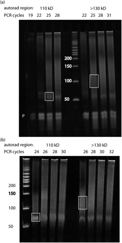
Two examples of RT-PCR from Ago HITS-CLIP experiments are shown, using samples from mouse T-cells (a) and mouse brain (b). In each case the 110 kD and >130 kD complexes were processed separately after isolation of RNA from the nitrocellulose membrane. PCR cycle numbers for each reaction are indicated above the gel. DNA size markers are indicated in bp. White boxes indicate gel regions that were excised and processed for high-throughput sequencing, as described in Anticipated Results. The ‘P’ in (a) indicates ‘primer-only’ products running below 50 bp, emphasizing the need for size selection and gel purification of appropriately sized products at this step. Primer-only products were run out of the gel in (b). Note that for the 110 kD complex, robust amplification of the ∼60 bp miRNA-dependent product occurs at earlier PCR cycles than for the >130 kD complex. Similarly, mRNA-dependent products, ideally a diffuse smear in the range from 85-110 bp, are enriched in the >130 kD complex. There is substantial cross-contamination between these populations, the degree of which varies according the resolution achieved at the SDS-PAGE step. However, we have found that separate, parallel isolation of these populations achieves higher complexity of mRNA tags, which represents a much more complex pool of sequences than the miRNA tags. Finally, note that products were excised from the lowest PCR cycles tested that gave robust signal. Plateaued signal and upward shift in modal size are indications of overamplification. Overamplification of tags, even by 1-2 cycles, can substantially reduce tag complexity.

Optimal amplification

In determining optimal PCR cycle number, the goal is the lowest level of amplification yielding sufficient material to move forward (Fig. 3). As a rule, if products are readily visible by eye upon UV illumination (i.e. without camera exposure), there is sufficient material to proceed. The integrated signal of PCR products at step 72 should scale linearly with PCR cycle number; plateaued signal indicates that the PCR is outside the linear range and products are overamplified. Other indications of overamplification include a ‘bandy’ pattern rather than a diffuse smear, or an upward size-shift relative to lower cycle numbers. Reactions within the linear PCR range, but with the lowest possible cycle number, should be purified at steps 72-74.

Similar samples (e.g., biologic replicates) should amplify in a similar range within and across experiments. However, because of low RT input and extensive processing, there may be some variability. For this reason, we empirically test a range of PCR cycles for each sample, even among replicates. As the protocol is optimized, it is likely that a finer range of PCR cycles can be tested and applied in future experiments. For example, Nova CLIP’d from ∼100mg of neonate mouse cortex typically has an optimal cycle number from 21-24 cycles. For Ago CLIP’d from similar material, miRNA tags will typically amplify between 24-26 cycles, while mRNA tags will amplify later, from 26-30 cycles.

Analysis for contamination

The appearance of products in –RT control samples may indicate DNA contamination of samples or reagents. Of particular concern are products that ‘look like’ those appearing in the +RT samples (i.e. similar size and, most ominously, in a similar amplification range). If such products appear in a –RT control sample, we recommend abandoning the corresponding +RT sample. Importantly, not all forms of contamination can be identified at this stage. Only adapter-containing DNA contaminants, introduced by sample cross-contamination or carry-over from prior experiments, will give products in a –RT control. A more general discussion of contamination appears below. Important points to consider in interpreting –RT controls include the following:

• To properly compare +RT and –RT samples, it is essential to examine reactions that have undergone similar amplification. If RNA was evenly divided between +RT and –RT samples at step 53, reactions of the same cycle number can be compared directly. If less RNA was used in –RT samples, PCR cycles must be adjusted upward accordingly for a fair comparison. For example, if 80% of RNA was used for +RT and 20% for –RT, –RT reactions should be run 2 additional cycles to compare fairly to corresponding +RT reactions. This is not a fully justified assumption, because PCR will not always scale linearly with very low amounts of input material. Therefore, we often examine –RT reactions several cycles beyond the range tested for +RT samples when input RNA is divided unevenly.

• If products appear only at late PCR cycles in –RT controls, it could indicate low levels of DNA contamination. The decision to move forward in this case is at the discretion of the investigator. A gap of 10 cycles between +RT and –RT samples (indicating 1 in every 2¹⁰, or 0.1%, contamination) will be acceptable in many circumstances, whereas a gap of 3 to 4 cycles is far more worrisome. Given the expense and time required to produce and analyze high-throughput sequencing results, we exercise extreme caution in making these judgements.

• It is possible for primer-dependent products to appear in –RT controls, sometimes as a primer-dimer or ‘ladder’. These products do not doom the experiment, as long as they are absent from +RT samples. If you suspect primer-dependent products, this can be confirmed by TOPO-TA cloning and standard DNA sequencing. We speculate, but can not prove, that such primer-dependent products are sometimes more favored in the absence of template. A ‘no template’ control (see optional portion of step 60) can be helpful in identifying primer-dependent bands.

Analysis of Second PCR (to add adapters) (step 84)

The results of the second PCR to add sequencing adapters should be evaluated to confirm correct product size and to determine optimal amplification. Contamination at this stage is a lesser concern than above, because the input material is far more abundant and requires less PCR amplification. Adapter sequences in primers SP5 and SP3 are 36 and 21 nt, respectively, adding a total of 57 bp to the products isolated at step 72. Products in the range of 80-120 bp will therefore yield a smear from ∼147-177 bp here. As in step 72, isolate the lowest cycle-number reactions with adequate product to proceed. Generally, products readily visible by eye upon UV illumination (i.e. without prolonged camera exposure) will yield sufficient material after gel purification for sequencing. In practice, it may be helpful to isolate products from two or more reactions, and proceed with the least-amplified sample with sufficient yield. Consult your sequencing facility in determining the amount of product that is required for analysis. As in the first PCR, plateaued signal, a ‘bandy’ pattern rather than a diffuse smear, or an upward size-shift relative to lower cycle numbers are signs of overamplification that should be avoided.

Contamination of Samples

Unfortunately, HITS-CLIP and other adapter-mediated PCR protocols are highly vulnerable to contamination because even vanishingly minute amounts of contaminants can be efficiently amplified. As a general measure, scrupulous attention to reagent quality is essential. To this end, we frequently replace inexpensive reagents (e.g., ethanol, IP buffers, and water), and aliquot more expensive reagents (e.g., enzyme buffers, dNTPs, primers) for single time use. In addition, pipet tips with aerosol filters should be used at all stages. Finally, equipment such as gel apparatuses that contact adapter-containing DNA or RNA should be decontaminated regularly with diluted bleach.

Two major types of contaminants are most common: 1.) adapter-containing DNA products, introduced at any stage, and 2.) undesired sources of RNA, introduced at any stage prior to RT.

DNA contaminants

DNA contaminants are likely to arise from cross contamination between samples or carry-over from prior experiments. These contaminants can be introduced at any stage prior to PCR, and are especially dangerous due to their inherent stability on surfaces and elsewhere. The DNAse treatment at step 49, after 5′ linker ligation, is meant to destroy potential DNA contaminants prior to RT-PCR. In addition, analysis of –RT controls is intended to diagnose DNA contamination.

RNA contaminants

RNA contaminants can take several forms. Accidental introduction of any RNA prior to linker ligation will lead to false identification of cross-linked RNA tags. In addition, cross-contamination or carry-over of linker-containing RNAs can occur at any stage prior to RT, with the same result. These forms of contamination can not be identified with –RT controls. As a countermeasure to this form of contamination, we have begun to use 5′ RNA linkers containing short 2-3 nucleotide ‘indexes’ to uniquely identify samples. An example of our 5′ linker RL5D follows containing a dinucleotide ‘CA’ index:

5′-OH AGG GAG GAC GAU GCG GCA r(N)r(N) r(N)r(N)G 3′-OH

Note that this ‘index’ is distinct from the degenerate barcodes in the 5′ linker used to collapse PCR duplicates. We rotate the use of different indexed 5′ linkers, so that cross-contaminants can be easily filtered during bioinformatic analysis. This strategy has the added benefit of allowing multiplexed sequencing analysis of samples. However, this measure will not identify contaminants introduced prior to 5′ linker ligation (step 47). It is less straightforward to incorporate indexes into the 3′ linker because for many tags, sequencing will not reach the 3′ end due to variable tag length. Use of a pair-end sequencing strategy would make the use of indexed 3′ linkers possible, but is more expensive and would require re-design of the adapter sequences described here.

In addition to spurious sources of RNA contamination, experimental sources such as co-purifying RNABPs are possible culprits. Instructions for the diagnosis and treatment of these contaminants is described in ‘Anticipated Results’ for SDS-PAGE/autorad results.

TROUBLESHOOTING

Troubleshooting advice can be found in Table 2.

Table 2.

Troubleshooting.

Step	Problem	Possible reason	Solution
34 and 37	No signal on autorad (step 34) and/or no depletion of antigen in post-IP fraction (step 37)	Failed or inefficient IP	Change antibodies or reduce IP stringency.
34 and 37	No signal on autorad (step 34), but antigen was depleted from post-IP fraction (step 37)	Post-IP washes too stringent	Reduce wash stringency.
34	High background signal on autorad (e.g., in control IgG or samples lacking RNABP)	IPs are ‘dirty’	Increase wash stringency. 2. Reduce sample input. 3. Reduce IP time or perform IP at room temperature.
34	Bands of unexpected size in ‘over-digested’ control that smear upward in partially digested samples	Co-purifying RNABP	Confirm if protein is an unknown isoform or degradation product of RNABP of interest Modify conditions (e.g., RNAse, gel percentage and run time, and excised nitrocellulose region) to minimize contamination.
34	Bands of unexpected size in ‘over-digested’ control that does not smear upward in partially digested samples	Co-purifying protein, not RNABP	Not a cause for concern.
34	‘Partially’ digested samples run as sharp band, at or near overdigested control	Too much RNAse	Decrease RNAse
34	Majority of signal in partially digested samples is > 20-30 kD above the overdigested control	Too little RNAse digestion	Increase RNAse dose.
72	No PCR products in +RT samples	1. Failed 3′ linker ligation 2. RNA not efficiently extracted from nitrocellulose membrane 3. Failed 5′ linker ligation 4. Failed RT	Track 3′ ligation using 32P- labeled 3′ linker (L32) instead of direct PNK labeling, according to Box 1. Confirm extraction of hot RNA with Geiger counter or scintillation counter (Cerenkov counts) after precipitation (step 52) Use pure (unsupported) nitrocellulose for transfer (step 29). Repeat 5′ ligation with more input RNA. Repeat RT with more input RNA
72	Appearance of products in –RT controls	1. DNA contamination 2. Primer-dependent products	Replace reagents and decontaminate all work surfaces and equipment with 10% bleach. Use aerosol filter tips at all steps. Perform ‘no template’ controls to identify possible primer-dependent products. Avoid these products during size selection.
72	PCR products appear at late PCR cycle number (>32) and are ‘bandy’ versus smear	Preferential amplification of specific products, due to insufficient input from RT	Increase input material
72	PCR products are smaller (<80 bp) than expected	RNA tags are small, possibly due to overdigestion with RNAse	Reduce RNAse concentration at steps 10 and 11. Cut from higher region of nitrocellulose at step 36.
72 and 84	PCR products are overamplified (i.e. plateaued signal, ‘bandy’ pattern versus smear, or upward size shift	PCR cycle number too high	Reduce PCR cycles
90	No or all reads pass filtering of quality scores	Type of quality score encoding is not specified correctly	Specify through option -if solexa or -if sanger
96,98,99,103,104	Insufficient memory	The input bed file is too large to be loaded into the memory at once	run the command line with option -big
96	The script reports errors or produce unexpected results	The structure of read IDs is not following the required format, and/or the number of substitutions is not recorded in the 5th column	The format of the ID is original ID#copy number#random barcode; record the number of substitutions in the 5th column of the tag BED file
98	CLIP tag distribution is very diffuse	Low stringency filtering in step 90, or alignment in step 91 (more likely)	Consider suggestions for step 97
98	CLIP tag distribution is very spiky	Duplicates are not collapsed properly in step 97	Consider suggestions in step 97
104	Script complains of inconsistency of files and ends unexpectedly	Mutations in non-unique tags are not removed properly	Revisit step 101
109,110	Motif frequency lower than expected	Low signal-to-noise of experiment, or the strand of sequences are not correct	For the latter, make sure the sequences of the sense strand obtained

References

- 1.Czech B, Hannon GJ. Small RNA sorting: matchmaking for Argonautes. Nat Rev Genet. 2011;12:19–31. doi: 10.1038/nrg2916. [DOI] [PMC free article] [PubMed] [Google Scholar]
- 2.Joshua-Tor L, Hannon GJ. Ancestral roles of small RNAs: an Ago-centric perspective. Cold Spring Harb Perspect Biol. 2011;3:a003772. doi: 10.1101/cshperspect.a003772. [DOI] [PMC free article] [PubMed] [Google Scholar]
- 3.Fabian MR, Sonenberg N, Filipowicz W. Regulation of mRNA translation and stability by microRNAs. Annu Rev Biochem. 2010;79:351–379. doi: 10.1146/annurev-biochem-060308-103103. [DOI] [PubMed] [Google Scholar]
- 4.Chi SW, Zang JB, Mele A, Darnell RB. Argonaute HITS-CLIP decodes microRNA-mRNA interaction maps. Nature. 2009;460:479–486. doi: 10.1038/nature08170. [DOI] [PMC free article] [PubMed] [Google Scholar]
- 5.Gaken J, et al. A functional assay for microRNA target identification and validation. Nucleic Acids Res. 2012;40:e75. doi: 10.1093/nar/gks145. [DOI] [PMC free article] [PubMed] [Google Scholar]
- 6.Bartel DP. MicroRNAs: target recognition and regulatory functions. Cell. 2009;136:215–233. doi: 10.1016/j.cell.2009.01.002. [DOI] [PMC free article] [PubMed] [Google Scholar]
- 7.Baek D, et al. The impact of microRNAs on protein output. Nature. 2008;455:64–71. doi: 10.1038/nature07242. [DOI] [PMC free article] [PubMed] [Google Scholar]
- 8.Chi SW, Hannon GJ, Darnell RB. An alternative mode of microRNA target recognition. Nat Struct Mol Biol. 2012;19:321–327. doi: 10.1038/nsmb.2230. [DOI] [PMC free article] [PubMed] [Google Scholar]
- 9.Ule J, Jensen K, Mele A, Darnell RB. CLIP: a method for identifying protein-RNA interaction sites in living cells. Methods. 2005;37:376–386. doi: 10.1016/j.ymeth.2005.07.018. [DOI] [PubMed] [Google Scholar]
- 10.Zhang C, Darnell RB. Mapping in vivo protein-RNA interactions at single-nucleotide resolution from HITS-CLIP data. Nat Biotechnol. 2011;29:607–614. doi: 10.1038/nbt.1873. [DOI] [PMC free article] [PubMed] [Google Scholar]
- 11.Granneman S, Kudla G, Petfalski E, Tollervey D. Identification of protein binding sites on U3 snoRNA and pre-rRNA by UV cross-linking and high-throughput analysis of cDNAs. Proc Natl Acad Sci U S A. 2009;106:9613–9618. doi: 10.1073/pnas.0901997106. [DOI] [PMC free article] [PubMed] [Google Scholar]
- 12.Ule J, et al. Nova regulates brain-specific splicing to shape the synapse. Nat Genet. 2005;37:844–852. doi: 10.1038/ng1610. [DOI] [PubMed] [Google Scholar]
- 13.Ule J, Darnell RB. RNA binding proteins and the regulation of neuronal synaptic plasticity. Curr Opin Neurobiol. 2006;16:102–110. doi: 10.1016/j.conb.2006.01.003. [DOI] [PubMed] [Google Scholar]
- 14.Ule J, et al. An RNA map predicting Nova-dependent splicing regulation. Nature. 2006;444:580–586. doi: 10.1038/nature05304. [DOI] [PubMed] [Google Scholar]
- 15.Darnell RB. HITS-CLIP: panoramic views of protein-RNA regulation in living cells. Wiley Interdiscip Rev RNA. 2010;1:266–286. doi: 10.1002/wrna.31. [DOI] [PMC free article] [PubMed] [Google Scholar]
- 16.Urlaub H, Hartmuth K, Luhrmann R. A two-tracked approach to analyze RNA-protein crosslinking sites in native, nonlabeled small nuclear ribonucleoprotein particles. Methods. 2002;26:170–181. doi: 10.1016/S1046-2023(02)00020-8. [DOI] [PubMed] [Google Scholar]
- 17.Ule J, et al. CLIP identifies Nova-regulated RNA networks in the brain. Science. 2003;302:1212–1215. doi: 10.1126/science.1090095. [DOI] [PubMed] [Google Scholar]
- 18.Licatalosi DD, et al. HITS-CLIP yields genome-wide insights into brain alternative RNA processing. Nature. 2008;456:464–469. doi: 10.1038/nature07488. [DOI] [PMC free article] [PubMed] [Google Scholar]
- 19.Licatalosi DD, Darnell RB. RNA processing and its regulation: global insights into biological networks. Nat Rev Genet. 2010;11:75–87. doi: 10.1038/nrg2673. [DOI] [PMC free article] [PubMed] [Google Scholar]
- 20.Sanford JR, et al. Splicing factor SFRS1 recognizes a functionally diverse landscape of RNA transcripts. Genome Res. 2009;19:381–394. doi: 10.1101/gr.082503.108. [DOI] [PMC free article] [PubMed] [Google Scholar]
- 21.Tollervey JR, et al. Characterizing the RNA targets and position-dependent splicing regulation by TDP-43. Nat Neurosci. 2011 doi: 10.1038/nn.2778. [DOI] [PMC free article] [PubMed] [Google Scholar]
- 22.Darnell JC, et al. FMRP Stalls Ribosomal Translocation on mRNAs Linked to Synaptic Function and Autism. Cell. 2011;146:247–261. doi: 10.1016/j.cell.2011.06.013. [DOI] [PMC free article] [PubMed] [Google Scholar]
- 23.Racca C, et al. The neuronal splicing factor Nova co-localizes with target RNAs in the dendrite. Front Neural Circuits. 2010;4:5. doi: 10.3389/neuro.04.005.2010. [DOI] [PMC free article] [PubMed] [Google Scholar]
- 24.Yano M, Hayakawa-Yano Y, Mele A, Darnell RB. Nova2 regulates neuronal migration through an RNA switch in disabled-1 signaling. Neuron. 2010;66:848–858. doi: 10.1016/j.neuron.2010.05.007. [DOI] [PMC free article] [PubMed] [Google Scholar]
- 25.Xue Y, et al. Genome-wide analysis of PTB-RNA interactions reveals a strategy used by the general splicing repressor to modulate exon inclusion or skipping. Mol Cell. 2009;36:996–1006. doi: 10.1016/j.molcel.2009.12.003. [DOI] [PMC free article] [PubMed] [Google Scholar]
- 26.Licatalosi DD, et al. Ptbp2 represses adult-specific splicing to regulate the generation of neuronal precursors in the embryonic brain. Genes Dev. 2012;26:1626–1642. doi: 10.1101/gad.191338.112. [DOI] [PMC free article] [PubMed] [Google Scholar]
- 27.Mukherjee N, et al. Integrative Regulatory Mapping Indicates that the RNA-Binding Protein HuR Couples Pre-mRNA Processing and mRNA Stability. Mol Cell. 2011;43:327–339. doi: 10.1016/j.molcel.2011.06.007. [DOI] [PMC free article] [PubMed] [Google Scholar]
- 28.Lebedeva S, et al. Transcriptome-wide Analysis of Regulatory Interactions of the RNA-Binding Protein HuR. Mol Cell. 2011;43:340–352. doi: 10.1016/j.molcel.2011.06.008. [DOI] [PubMed] [Google Scholar]
- 29.Ince-Dunn G, et al. Neuronal Elav-like (Hu) Proteins Regulate RNA Splicing and Abundance to Control Glutamate Levels and Neuronal Excitability. Neuron. 2012;75:1067–1080. doi: 10.1016/j.neuron.2012.07.009. [DOI] [PMC free article] [PubMed] [Google Scholar]
- 30.Wang Z, et al. iCLIP predicts the dual splicing effects of TIA-RNA interactions. PLoS Biol. 2010;8:1–16. doi: 10.1371/journal.pbio.1000530. [DOI] [PMC free article] [PubMed] [Google Scholar]
- 31.Polymenidou M, et al. Long pre-mRNA depletion and RNA missplicing contribute to neuronal vulnerability from loss of TDP-43. Nat Neurosci. 2011;14:459–468. doi: 10.1038/nn.2779. [DOI] [PMC free article] [PubMed] [Google Scholar]
- 32.Konig J, et al. iCLIP reveals the function of hnRNP particles in splicing at individual nucleotide resolution. Nat Struct Mol Biol. 2010;17:909–915. doi: 10.1038/nsmb.1838. [DOI] [PMC free article] [PubMed] [Google Scholar]
- 33.Yeo GW, et al. An RNA code for the FOX2 splicing regulator revealed by mapping RNA-protein interactions in stem cells. Nat Struct Mol Biol. 2009;16:130–137. doi: 10.1038/nsmb.1545. [DOI] [PMC free article] [PubMed] [Google Scholar]
- 34.Charizanis K, et al. Muscleblind-like 2-Mediated Alternative Splicing in the Developing Brain and Dysregulation in Myotonic Dystrophy. Neuron. 2012;75:437–450. doi: 10.1016/j.neuron.2012.05.029. [DOI] [PMC free article] [PubMed] [Google Scholar]
- 35.Leung AK, et al. Genome-wide identification of Ago2 binding sites from mouse embryonic stem cells with and without mature microRNAs. Nat Struct Mol Biol. 2011;18:237–244. doi: 10.1038/nsmb.1991. [DOI] [PMC free article] [PubMed] [Google Scholar]
- 36.Loeb GB, et al. Transcriptome-wide miR-155 Binding Map Reveals Widespread Noncanonical MicroRNA Targeting. Mol Cell. 2012;48:760–770. doi: 10.1016/j.molcel.2012.10.002. [DOI] [PMC free article] [PubMed] [Google Scholar]
- 37.Riley KJ, et al. EBV and human microRNAs co-target oncogenic and apoptotic viral and human genes during latency. EMBO J. 2012;31:2207–2221. doi: 10.1038/emboj.2012.63. [DOI] [PMC free article] [PubMed] [Google Scholar]
- 38.Zisoulis DG, et al. Comprehensive discovery of endogenous Argonaute binding sites in Caenorhabditis elegans. Nat Struct Mol Biol. 2010;17:173–179. doi: 10.1038/nsmb.1745. [DOI] [PMC free article] [PubMed] [Google Scholar]
- 39.Hafner M, et al. Transcriptome-wide identification of RNA-binding protein and microRNA target sites by PAR-CLIP. Cell. 2010;141:129–141. doi: 10.1016/j.cell.2010.03.009. [DOI] [PMC free article] [PubMed] [Google Scholar]
- 40.Mili S, Steitz JA. Evidence for reassociation of RNA-binding proteins after cell lysis: implications for the interpretation of immunoprecipitation analyses. RNA. 2004;10:1692–1694. doi: 10.1261/rna.7151404. [DOI] [PMC free article] [PubMed] [Google Scholar]
- 41.Kishore S, et al. A quantitative analysis of CLIP methods for identifying binding sites of RNA-binding proteins. Nat Methods. 2011;8:559–564. doi: 10.1038/nmeth.1608. [DOI] [PubMed] [Google Scholar]
- 42.Kemeny-Beke A, et al. Antiproliferative effect of 4-thiouridylate on OCM-1 uveal melanoma cells. Eur J Ophthalmol. 2006;16:680–685. [PubMed] [Google Scholar]
- 43.Burger K, et al. 4-thiouridine inhibits rRNA synthesis and causes a nucleolar stress response. RNA Biol. 2013;10 doi: 10.4161/rna.26214. [DOI] [PMC free article] [PubMed] [Google Scholar]
- 44.Khan AA, et al. Transfection of small RNAs globally perturbs gene regulation by endogenous microRNAs. Nat Biotechnol. 2009;27:549–555. doi: 10.1038/nbt.1543. [DOI] [PMC free article] [PubMed] [Google Scholar]
- 45.Hafner M, et al. RNA-ligase-dependent biases in miRNA representation in deep-sequenced small RNA cDNA libraries. RNA. 2011;17:1697–1712. doi: 10.1261/rna.2799511. [DOI] [PMC free article] [PubMed] [Google Scholar]
- 46.Zhuang F, Fuchs RT, Sun Z, Zheng Y, Robb GB. Structural bias in T4 RNA ligase-mediated 3′-adapter ligation. Nucleic Acids Res. 2012;40:e54. doi: 10.1093/nar/gkr1263. [DOI] [PMC free article] [PubMed] [Google Scholar]
- 47.Harlow E, Lane D. Antibodies, a laboratory manual. Cold Spring Harbor Laboratory; Cold Spring Harbor, New York: 1988. [Google Scholar]
- 48.Green M, Sambrook J, editors. Mapping of in vivo RNA binding sites by UV-crosslinking immuopreciptiation (CLIP) Cold Spring Harbor Laboratory Press; 2012. [Google Scholar]
- 49.Parker JS. How to slice: snapshots of Argonaute in action. Silence. 2010;1:3. doi: 10.1186/1758-907X-1-3. [DOI] [PMC free article] [PubMed] [Google Scholar]
- 50.Ren B, et al. Genome-wide location and function of DNA binding proteins. Science. 2000;290:2306–2309. doi: 10.1126/science.290.5500.2306. [DOI] [PubMed] [Google Scholar]
- 51.Granneman S, Petfalski E, Swiatkowska A, Tollervey D. Cracking pre-40S ribosomal subunit structure by systematic analyses of RNA-protein cross-linking. EMBO J. 2010;29:2026–2036. doi: 10.1038/emboj.2010.86. [DOI] [PMC free article] [PubMed] [Google Scholar]
- 52.Bohnsack MT, et al. Prp43 bound at different sites on the pre-rRNA performs distinct functions in ribosome synthesis. Mol Cell. 2009;36:583–592. doi: 10.1016/j.molcel.2009.09.039. [DOI] [PMC free article] [PubMed] [Google Scholar]
- 53.Wang ET, et al. Transcriptome-wide Regulation of Pre-mRNA Splicing and mRNA Localization by Muscleblind Proteins. Cell. 2012;150:710–724. doi: 10.1016/j.cell.2012.06.041. [DOI] [PMC free article] [PubMed] [Google Scholar]
- 54.Cho J, et al. LIN28A is a suppressor of ER-associated translation in embryonic stem cells. Cell. 2012;151:765–777. doi: 10.1016/j.cell.2012.10.019. [DOI] [PubMed] [Google Scholar]
- 55.Rhead B, et al. The UCSC Genome Browser database: update 2010. Nucleic Acids Res. 2010;38:D613–9. doi: 10.1093/nar/gkp939. [DOI] [PMC free article] [PubMed] [Google Scholar]
- 56.Bailey TL, Elkan C. Fitting a mixture model by expectation maximization to discover motifs in biopolymers. Proc Int Conf Intell Syst Mol Biol. 1994;2:28–36. [PubMed] [Google Scholar]
- 57.Tempel S. Using and understanding RepeatMasker. Methods Mol Biol. 2012;859:29–51. doi: 10.1007/978-1-61779-603-6_2. [DOI] [PubMed] [Google Scholar]
- 58.Sugimoto Y, et al. Analysis of CLIP and iCLIP methods for nucleotide-resolution studies of protein-RNA interactions. Genome Biol. 2012;13:R67. doi: 10.1186/gb-2012-13-8-r67. [DOI] [PMC free article] [PubMed] [Google Scholar]