Quantitative assessment of automatic reconstructions of branching systems obtained from laser scanning

Abstract

Background and Aims

Automatic acquisition of plant architecture is a major challenge for the construction of quantitative models of plant development. Recently, 3-D laser scanners have made it possible to acquire 3-D images representing a sampling of an object's surface. A number of specific methods have been proposed to reconstruct plausible branching structures from this new type of data, but critical questions remain regarding their suitability and accuracy before they can be fully exploited for use in biological applications.

Methods

In this paper, an evaluation framework to assess the accuracy of tree reconstructions is presented. The use of this framework is illustrated on a selection of laser scans of trees. Scanned data were manipulated by experienced researchers to produce reference tree reconstructions against which comparisons could be made. The evaluation framework is given two tree structures and compares both their elements and their topological organization. Similar elements are identified based on geometric criteria using an optimization algorithm. The organization of these elements is then compared and their similarity quantified. From these analyses, two indices of geometrical and structural similarities are defined, and the automatic reconstructions can thus be compared with the reference structures in order to assess their accuracy.

Key Results

The evaluation framework that was developed was successful at capturing the variation in similarities between two structures as different levels of noise were introduced. The framework was used to compare three different reconstruction methods taken from the literature, and allowed sensitive parameters of each one to be determined. The framework was also generalized for the evaluation of root reconstruction from 2-D images and demonstrated its sensitivity to higher architectural complexity of structure which was not detected with a global evaluation criterion.

Conclusions

The evaluation framework presented quantifies geometric and structural similarities between two structures. It can be applied to the characterization and comparison of automatic reconstructions of plant structures from laser scanner data and 2-D images. As such, it can be used as a reference test for comparing and assessing reconstruction procedures.

INTRODUCTION

The acquisition of accurate models of real plants is a time-consuming task and a major bottleneck for the construction of quantitative models of plant development. Recently, 3-D laser scanners have made it possible to acquire 3-D images representing object surface samplings. To process this new type of data, dedicated automatic reconstruction methods have been developed (Alexa et al., 2003). Although successful in most applications, such as urban geometry (Hu et al., 2003), these methods usually fail on botanical structures as they frequently contain a complex set of irregular and branching surfaces distributed in space with varying orientations. A number of specific methods have been proposed to reconstruct plausible branching structures from laser data. However, no comparative evaluation was carried out to assess the resulting reconstructions. In particular, methods to evaluate the structural accuracy of the architecture are still lacking. The definition of such a structural evaluation method is the topic of this work.

Xu et al. (2007), who extended the method of Verroust and Lazarus (2000), proposed the first notable reconstruction method for branching structures. Points from the laser scans are first connected to their k closest neighbours to form a graph (called the Riemannian graph). The distance between any two points is then defined as the length of the shortest path between these points on the graph. Next, the graph is segmented into clusters of points according to the distance from a specified root point. Finally, cluster centres are used to generate the tree skeleton.

In subsequent work, Yan et al. (2009) proposed that the point segmentation could be performed with a hierarchical cylinder fitting using k-means clustering. Raumonen et al. (2013) proposed to fit cylinders by aggregating small patches of points. Livny et al. (2010) used a series of global optimization procedures to reconstruct major skeletal branches. In this approach, the longest paths in the Riemannian graph are identified and used to align and to prune out the points. The remaining paths form the skeleton of the tree. As an alternative, a series of methods were developed based on the concept of space colonization (Runions et al., 2007). This consists of running a simulated growing tree process attracted by a set of points that represent the volume of the plant. This approach was first exploited by Coté et al. (2009) to generate realistic foliage of a tree from laser scans. Preuksakarn et al. (2010) extended this idea to follow the point patterns of the scans precisely to reconstruct the skeleton of trees.

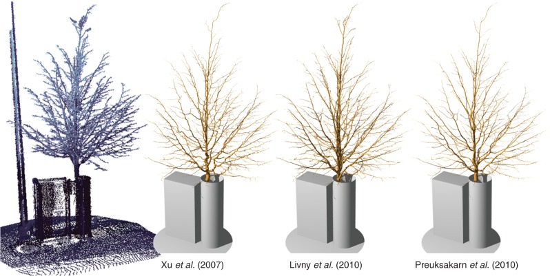
While these methods produce visually realistic structures (Fig. 1), their respective accuracy and relative merits are still difficult to assess. Nevertheless, such an evaluation is of major importance for further exploitation of reconstructed models in biological applications. This work aims to propose a computational framework to evaluate structures reconstructed from laser scanner data. For this purpose, we first developed a software tool that allows experienced researchers to define a tree skeleton manually from the point cloud. Using these expert-defined structures, which are then considered as a reference, we then propose a comparison framework to quantify similarities and differences between two structures. The framework takes into account both the geometry and the organization of the branching elements. Such an evaluation framework makes it possible to compare an automatic reconstruction with a reference structure to assess its structural accuracy. As a result, we used it to design a first evaluation procedure of different reconstruction methods found in the literature. To show the generality of our method, we also apply it on a large data set of root structures reconstructed from 2-D images.

Fig. 1.

A scanned tree and its reconstructions according to different methods found in the literature.

MATERIALS AND METHODS

Scanning material

In this study, we use laser scans from two lime trees growing in the streets of Helsinki, Finland, which were obtained from a Leica Geosystems HDS 2500 laser scanner. We also use a scan of a cherry tree near Clermont-Ferrand, France, obtained using a Leica Geosystems HDS 6200 laser scanner. Trees were scanned from three to four positions to reduce occlusions. The scanner specification gives a range of accuracy of 4 mm for the position of a point in space.

From these scanned trees, reference 3-D models were then built. To do this, we designed a visual editor that allows users to specify 3-D branching skeletons and asked experienced researchers to build reconstructed structures (Fig. 2). They started from preliminary automatic reconstructions that they corrected and completed using their expert knowledge of structures. Using the visual editor, these experts could edit the skeletal structure of each tree by adding, deleting, repositioning or reorganizing segments in the structure. Different visualization tools offered by the software made it possible to focus on specific locations, allowing straightforward identification of local branching configurations. The results are tree-like structures, whose nodes are associated with branch segments, and that represent the skeleton of the plant branching structure.

Fig. 2.

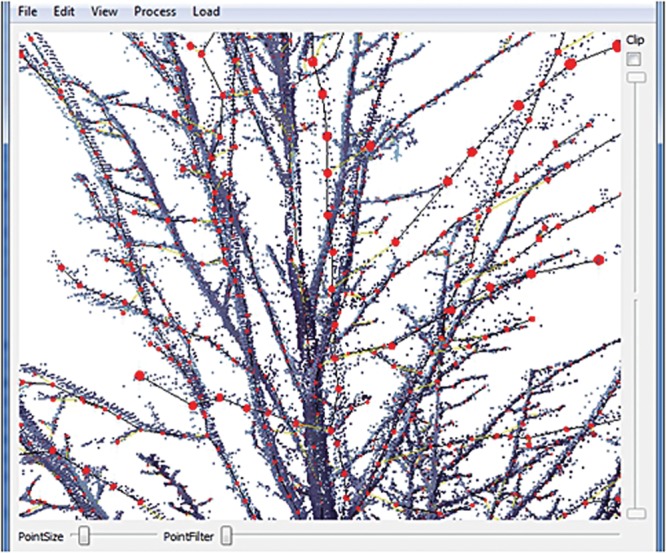
The software tool used by experienced researchers to create structures from laser data. Red spheres represent nodes of the structure. Sliders control the location and the size of the laser point display. The user can edit the plant structure by adding, deleting, moving or changing the properties of nodes.

These reference structures can be considered as the best possible reconstructions from the laser scans. However, because of occlusions and lower resolution in some parts of the scan images, for example at the top of the tree, even an expert cannot detect some components of the tree from the scans. To alleviate this difficulty, we also used a known structure that was virtually scanned. We used a virtual model of a walnut tree (Sinoquet et al., 1997), whose structure was first manually measured from a real tree using a magnetic 3-D digitizer (Polhemus 3Space Fastrak). This mock-up was virtually scanned using the Z-buffer computation capabilities of a computer graphics card. Using graphics cards, a discretization in terms of pixels with associated depth from a given point of view can be performed interactively on complex 3-D geometry.

On all of the input data mentioned above, we created reconstructions using our implementation of the methods of Xu et al. (2007), Preuksakarn et al. (2010) and Livny et al. (2010) (Fig. 1). These implementations are now part of the PlantGL open source library (Pradal et al., 2009) of the OpenAlea platform (Pradal et al., 2008).

Existing methods of reconstruction

Two classes of quantitative evaluation can be distinguished. The first one consists of summarizing an individual tree by a small number of global variables such as wood content, crown volume, amount of intercepted light from several directions, etc. The similarity between reconstructions is then measured as a distance between these synthetic variables.

As a first approach, our different reconstructions are compared with reference trees with such global indices. We compare the reconstructions with the original point sets by estimating the average distance of the points to the reconstructed models. We also compare the volume or total branch length between reconstructions and the reference structures that had been compiled by experts. While this gives a general assessment of the reconstruction quality, these indices give no information on the quality of the reconstructed topology.

A second class of evaluation consists of comparing in more detail the 3-D structure of the reconstructions using structural comparison tools. As a first test, we experimented with the edit distance proposed by Ferraro and Godin (2000). This distance is computed as the minimum cost of a sequence of edit operations that transforms an initial tree T₁ into a target tree T₂. Three edit operations are usually considered: substituting a vertex i of T₁ with a vertex j of T₂, deleting a vertex i in T₁ and inserting a vertex j in T₂. Each operation is associated with a cost that we parameterized according to geometric similarities between nodes. As a side product, the set of operations gives a mapping between elements of T₁ and T₂, the cost of the mapping being identical to the cost of the sequence of edit operations.

However, only mappings that preserve ancestor relationships between elements of the trees are considered by the method. As a result, although two trees might differ by a simple inversion of a branching structure position, this inversion may lead to a costly mapping between the trees, as illustrated in Fig. 3. This problem is critical since the exact location of branching points may be imprecise in scanner data due to partial occlusion. Thus, a new edit distance that limits the influence of branching errors is required to evaluate reconstructed structures from laser data.

Fig. 3.

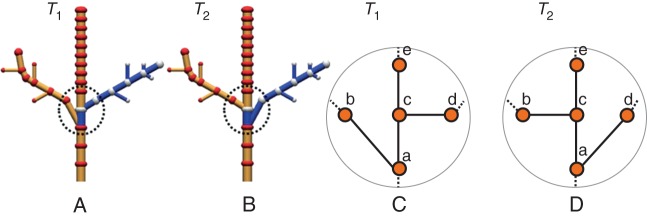
A comparison of two structures with a high degree of similarity. The only difference is the location of the branching point of the two laterals branches. Due to this simple inversion, the ancestor relationships between branching structures is not preserved. Using the comparison method of Ferraro and Godin (2000), the two right-hand branches are found to be significantly different. The cost used to parameterize the method for the substitution is set equal to the distance between positions of the nodes. Deletion and insertion costs are set to three times the average size of a node. (A, B) The two compared trees. The blue parts of the structures are not matched. (C, D) Zoom on the branches' connections on the trunk. A simple inversion of the connections at nodes a and c is introduced between T₁ and T₂.

A new comparison framework

To overcome the above limitation, we designed a less constrained comparison framework that makes it possible to detect similarities between structures even in the case of mismatched connections. For this purpose, a number of algorithmic steps are performed to estimate two indices that reflect both geometric and structural similarities (Fig. 4). First, the scales of representation of the compared trees T₁ and T₂ are homogenized. A mapping of their elements based on geometric criteria is then performed to determine similar elements. Finally, a mapping of the edges of the two structures is computed to quantify the similarity of their organization. From these mappings, two indices are estimated to quantify geometric and topological similarities. The different steps employed to compute these indices are presented in detail in the following sections.

Fig. 4.

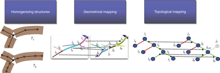
Our comparison framework makes it possible to estimate both geometrical and topological differences between structures. In a first step, both compared structure scales are homogenized. The elements of these structures are then compared based on geometric criteria to find similar elements. Finally, the topology of these elements is compared to quantify the similarity of their organization.

Homogenizing structures

Some arbitrary choices are made during the creation of a plant model from a laser scan, e.g. a reconstruction method or one produced by an expert (at a given resolution) may represent the same branch with a variable number of segments. A first problem thus consists of re-expressing the structures to compare in a common resolution (or scale).

A natural scale to consider is that of entire branches. However, in an automatically reconstructed structure, the continuity of the branches at branching points is difficult to determine (particularly in sympodial structures). This problem can be avoided by considering the scale of an inter-ramification branch unit (IBU) that consists of the linear parts of branches delineated by two consecutive branching points.

To create trees made of IBUs, we merged all the branch segments connecting any two branching points. For this, we performed a quotient operation on the detailed tree graph using the multiscale tree graph formalism proposed to represent plants (Godin and Caraglio, 1998). For each IBU, a skeleton curve is constructed as the union of its constituent segments. As a result, we get a tree graph T_i = <V_i, E_i> where V_i represents the set of IBUs and E_i is a set of edges represented by ordered pairs of IBUs and describing connections between IBUs. Each vertex is associated with a sequence of node positions representing the path of the segments constituting the IBU.

Geometrical mapping

Based on the homogenized structures, the comparison of the test and reference structures could then be carried out. In 3-D space, these two structures correspond to two sets of segments that may partially overlap, making it difficult to find exact correspondences between the test and the reference reconstructions. In practice, this association is often ambiguous and, for each segment of the test (respectively reference) structure, one can associate a list of candidate segments in the reference (respectively test) structure.

Let us call T₁ and T₂ the reference and test tree skeletons, respectively. For any pair of IBUs that can possibly be mapped from T₁ to T₂, we quantify the distance between these two IBUs as the Hausdorff distance between their skeleton curves. Let C_i and C_j be two skeletal polylines defined by the set of control points {Pⁱ_k, k ϵ [0,Nⁱ]} and {P^j_l, l ϵ [0,N ^j]}, respectively, and parameterized with an index u ϵ [0,1]. Actually, the control points represent the positions of the nodes that comprise the IBU. The Hausdorff distance of the segments is defined as

$$d_H(C_i,C_j)=\text{max}\{{\text{max}}_{k{ϵ[0,N}^i]}[d(P_i^k,C_j)],{\text{max}}_{\mathrm{l}{ϵ[0,N}^j]}[d(C_i,P_l^j)]\},$$

$$d(P_i,C_j)={\text{min}}_u(||P_i-C_j(u)||).$$

Intuitively, it represents the maximal deviation between the curves.

Using such a distance, the similarity between two elements can be quantified. However, finding the mapping that minimizes the overall distance between elements in T₁ to T₂ is a combinatorial problem. For instance, in Fig. 5, the element i₅ can potentially be mapped to j₄, j₅, j₆ and j₇; the element i₄ to j₂ and j₄; and so on. Obviously, an optimal solution would map i₄ to j₄ and i₅ to j₅ and j₆. Thus, ideally the assignment problem should map an element of T₁ to one or several elements of T₂ and, conversely, one element of T₂ should be mapped to one or several elements of T₁. However, in such a general form, the problem is NP-Hard (Zhang and Jiang, 1994). We thus decompose the problem into simpler sub-problems. We first use an optimization algorithm to find an optimal one-to-one mapping, i.e. for each element of T₁ finding the most similar element in T₂, and vice versa. Then we extend this mapping with configurations for multiple segments.

Fig. 5.

Example of geometrical comparison between elements of two structures.

In the mapping between the two structures, some elements in the reference skeleton may have no counterpart in the test skeleton, and vice versa (see j₇ in Fig. 5). In this case, we say that we have, respectively, a deletion or an insertion with respect to the reference structure. Specific deletion and insertion distances, denoted as d_H(C_i, θ) and d_H(θ, C_j) respectively, are assigned to these special mappings and are set equal to the length of the skeleton curve C_i of the IBU.

To determine an optimal one-to-one mapping, we define a valid mapping between T₁ and T₂ as a list of pairs M = {(i, j)}, with i ϵ T₁ U θ and j ϵ T₂ U θ such that for any i, j, k ≠ θ, if (i, j) and (i, k) are in M then j = k, and, reciprocally, if (i, j) and (k, j) are in M then i = k. A valid mapping M is associated with a cost d(M) defined as the sum of the cost of each individual mapping and of the deletions and insertions of nodes

$$d(M)={\mathrm{\Sigma }}_{(i,j)ϵM}{d}_H\left(C_{i,}{C}_j\right)$$

The comparison of our two skeletal structures thus comes down to finding the valid mapping M with minimal cost

$$M\ast ={\text{argmin}}_{M}d(M).$$

To solve this assignment problem, we use an optimal flow formulation (Fig. 6). For this, we define a bipartite graph made of two set of nodes {i ϵ T₁} and {j ϵ T₂} such that any node i is connected to its potential candidates in T₂ and, reciprocally, any node j is connected to its potential candidates in T₁. To decide whether a connection between any two nodes i and j should exist, we determine if these two elements can potentially be mapped. We check if the distance between their bounding boxes is less than a given threshold representing the maximal distance allowed between elements. A cost is then attached to these edges that corresponds to the distance between the curves of the connected nodes (Fig. 6). Note that two nodes θ_i and θ_j have been introduced to express the possibilities of deletion and insertion of nodes, with their corresponding costs as explained above. Two extra nodes s and t are added and represent source and sink for the flow which are linked to the set of nodes i and θ_i and to the set of nodes j and θ_j respectively. We define capacities of value 1 on edges connecting s with i and j with t. These capacities define the amount of flow that should pass on these edges. This ensures that the flow will be exactly 1 on these edges and thus define a valid mapping between nodes i and j. Edges between nodes i and j are given a maximum capacity of 1 and a minimal capacity of 0 to model possible matching between elements.

Fig. 6.

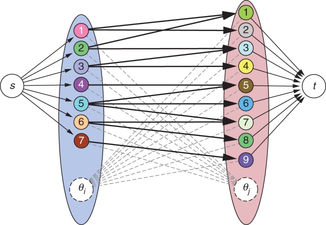
The optimal flow formulation of the mapping of the inter-ramification branch units (IBUs) of tree T₁ (left) onto the IBUs of tree T₂ (right). s represents the source and t the sink.

Finally, the minimal cost maximum flow is determined using Tarjan's extension (1983) of Edmonds and Karp's algorithm (1972). As a result, a maximum number of paths going from s to t are saturated, with the sum of the costs of their edges being minimal. Thus, a selection of edges that link nodes i to nodes j are saturated and can be interpreted as a one-to-one matching between the two sets of elements.

In the resulting optimal mapping M*, some elements may be deleted or inserted. However, some of these insertions/deletions may simply result from the fact that several segments in one tree altogether cover a single segment in the other tree. In this case, M* only contains a mapping from one of the small segments to the single segment and considers that all the other small segments have been deleted (or inserted). To take this property into account, a post-processing step refines the mapping produced from the previous step by testing and adding mapping configurations that include multiple segments. Each mapping of a node i with a node j is examined to check if one of the two elements has some neighbouring elements not assigned. If, for instance, i has such a neighbour k, the union of the skeleton of i and k is tested with the Hausdorff distance to the skeleton of j. If this distance value is less than the distance between i and j, the mapping is corrected and (i, j) is replaced by ((i, k), j) (i.e. j is mapped on both i and k). This procedure is repeated recursively to test any sequence of i or j, thus leading to a modified, more precise mapping between T₁ and T₂.

As a result of this mapping procedure, a geometric correspondence between elements is defined and can be quantified with the index

$$D_G(T_1,T_2)=\frac{\text{2}|M^{\ast }|}{|T_1|+|T_2|}.$$

Topological mapping

To evaluate the difference of topology between both structures, we then inspect whether their elements are connected in a similar way in their respective structures. We check if any relationship between two nodes i₁ and i₂ of the tree graph T₁ has a counterpart in T₂ that links the corresponding j₁ and j₂ elements (Fig. 7).

Fig. 7.

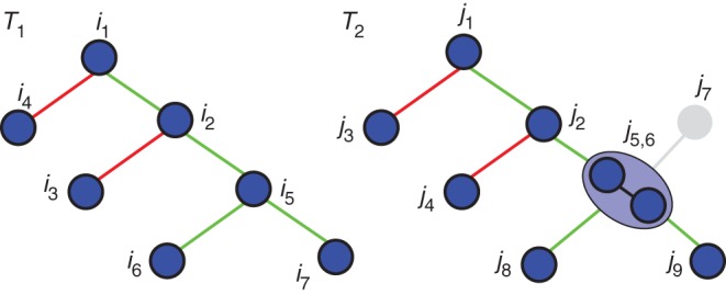
A comparison of the topologies of the two branching structures of Fig. 5. The graphs are first simplified, with j₇ being removed and j₅ and j₆ merged. Finally, all edges of T₁ are compared with their counterparts in T₂. For instance, the edge linking i₁ and i₂ has its counterpart between j₁ and j₂ and thus is said to be preserved and is represented in green. However, the edge between i₁ and i₄ has no counterpart between j₁ and j₄ and is represented in red.

To perform this evaluation, we first simplify the two tree graphs T₁ and T₂ to restrain them to nodes with counterparts in the other tree. Thus, we remove the non-matched elements [i.e. any element i such that (i, θ_j) ϵ M* and any element j such that (θ_i, j) ϵ M*]. For instance in Fig. 7, the node j₇ is removed since it is not matched to any node of T₁. To keep a valid tree graph structure, we then reconnect any node whose parent was removed to its first non-removed ancestor. Additionally, at the end of the procedure, M* contains mapping configurations that involve multiple elements. We simplify T₁ and T₂ by merging all sets of elements that are mapped all together into one unique element, i.e. if ((i₁, i₂, … ,i_n),j) ϵ M* then the set of elements (i₁, i₂, … ,i_n) is merged into a unique element i. This is illustrated visually in Fig. 7 with nodes j₅ and j₆. This results in two simplified tree graphs T′₁ and T′₂.

To check for topological similarity, we check all matching pairs (i, j) ϵ M*. Considering the edge e_i = (p_i, i) ϵ E′₁ of T′₁ (meaning that p_i is the parent of i in T′₁) and the edge e_j = (p_j, j) ϵ E₂ of T₂, if (p_i, p_j) ϵ M*, we say that the relationships e_i and e_j are preserved and (e_i, e_j) is included in the topological mapping M^T. Finally, we quantify the topological similarity between two structures with the normalized index

$$D_T(T_1^{\mathrm{\prime }},T_2^{\mathrm{\prime }})=\frac{2|M^T|}{|E_1|+|E_2|}.$$

RESULTS AND DISCUSSION

To validate this comparison framework, we performed a sensitivity analysis. We then used our framework to compare three different reconstruction methods described in the literature. Finally, to show the generality of our framework, we apply it to the reconstruction of root structures from photographs.

Sensitivity analysis of the similarity indices

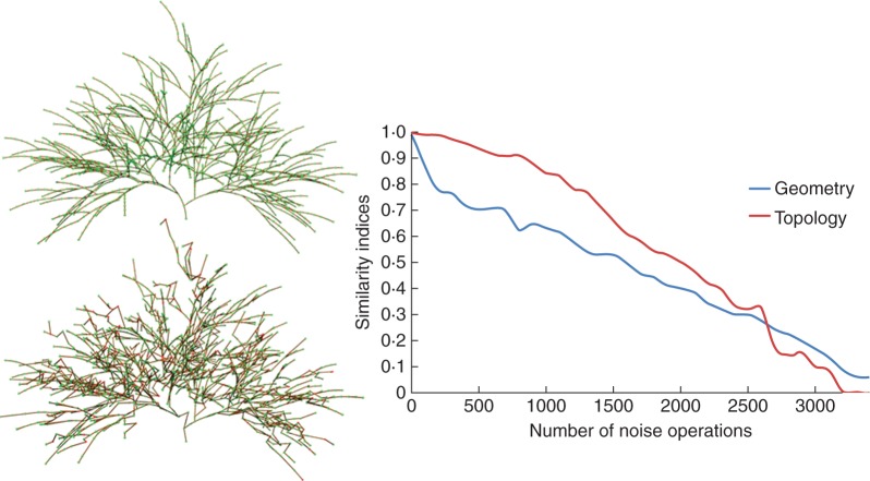
To analyse the performance of our new comparison metric, we applied it on structures with several levels of noise. On a simple synthetic reference structure of approx. 2200 nodes (Fig. 8, top), several levels of noise are introduced using three operators: an insertion operator that creates new nodes in the graph; a deletion operator that removes nodes; and a move operator that shifts the location of existing nodes. A sequence of noise operations is applied progressively to the reference structure. At each step, the geometrical and topological similarities between the reference and the noisy structure are computed using indices D_G and D_T. In a first test, the type of each noise operation in the sequence is chosen randomly and results in the graph of Fig. 8. An example of a generated structure with 1000 random noise operations is given in Fig. 8, bottom left. Without noise, the distances are equal to 1 and decrease progressively toward 0 with a close to linear behaviour. Similar results were achieved on different reference structures in our database (data not shown).

Fig. 8.

The geometrical and topological similarity assessed using indices D_G (geometry) and D_T (topology) between a reference structure and the same structure on which a number of random noise operations has been performed. The reference structure is shown at top left, and the structure after 1000 random noise operations is below it. The graph shows the values of D_G and D_T as functions of the different levels of noise.

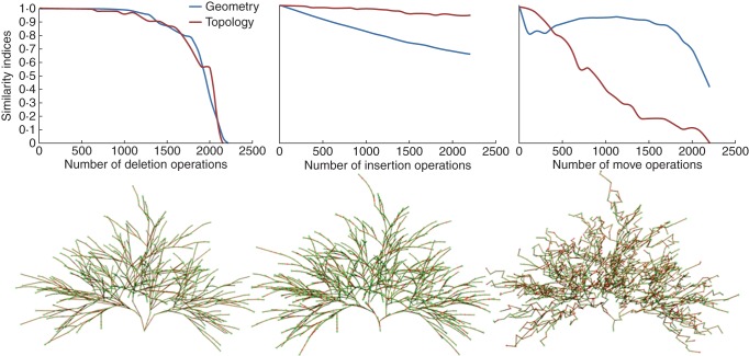
We then studied more precisely the effect of each type of noise operator (Fig. 9). First, we applied only the deletion operator (Fig. 9 left). Interestingly, after approx. 1200 nodes were deleted, the evaluation still gives a high degree of similarity (>0·9 for both D_G and D_T). In this phase, the deletions seem to be interpreted as a simplification of the structure. Our approach is not overly sensitive to this type of change thanks to the scale homogenization step that regroups sets of nodes into IBUs, representing more global components. Missing nodes simply change the local geometry of the IBUs, but the units will remain globally similar. For a greater number of deletions, certain IBUs have all their nodes removed. This changes drastically both the geometry and the topology of the plant and thus induces a rapid decrease of the indices in the second part of the graph. In a second step, we only performed insertions into the structure (Fig. 9, middle). In this case, the geometrical similarity slowly decreases while topological similarity stays close to 1. This can be explained in the following way. After insertion, the noisy structure contains two types of elements: the initial ones and the added ones. Because they are exactly similar, the initial elements of the noisy structure are matched onto the elements of the reference structure. The added elements do not have counterparts and thus are not matched, yet they still increase the total number of elements. Since the geometric similarity is a ratio between the number of matched elements and the total number of elements, its value decreases. This does not affect the topological similarity since this index considers only the matched elements.

Fig. 9.

An evaluation of the effect of each type of noise operation on the similarity indices. Deletion, insertion and move noise operations were tested separately, as indicated in the graph labels. The values of D_G (geometry) and D_T (topology) as a function of the number of performed noise operations are shown in the graphs, while the images illustrates the noise structures after 1000 operations.

Finally, the third test only applies node relocation operations to the structure (Fig. 9, right). The geometric similarity curve has three phases: a rapid decrease in the beginning, a constant phase until 1700 operations and again a rapid decrease at the end. The topological similarity decreases linearly. The relocation operation introduces some noise in the geometric mapping by changing the elements that are mapped. The use of the Hausdorff distance is sufficiently flexible that a moved element will be considered similar if it comes close enough to another element. However, their positions in the tree graph structure are different, and thus represent different topologies. This difference is reported by the constant decrease of the topological similarity index. In conclusion, these tests show that the two indices are able to report the geometric and structural difference between different tree structures correctly.

Comparative evaluation of the different methods in the literature

In this section, a first comparative study of three reconstruction methods M1 (after Xu et al., 2007), M2 (after Livny et al., 2010) and M3 (after Preuksakarn et al., 2010) is presented. For this, we re-implemented these methods by thoroughly following the description in the corresponding article. Note, however, that subtle differences may exist between our implementation and the authors' original implementation that may include specific optimizations that were not described. Additionally, all of the methods depend on a number of parameters. We did not make an extensive exploration of the parameter space for each reconstruction but rather tuned them by hand to obtain a visually good reconstruction. To evaluate the different methods, we compared the structure they produced with the structures reconstructed by the experienced researchers for three different scans of trees and the virtual walnut tree structure which was virtually scanned.

We first estimated three global criteria, whose results are presented in Table 1. For each reconstruction, the volume of the model, the cumulative length of all its branches and the average distance of the points of the scan to the skeleton are estimated. From this result, the behaviour of the different methods can thus be analysed in the following way. All reconstruction methods seem to underestimate the volume of the tree (7 % on average) and overestimate the total branch length (approx. 15 % for M1 and M3, and 70 % for M2). However, the total branch length is underestimated specifically for the virtual scan of the walnut tree. This may come from the smallest branches, which are difficult to perceive in the scans, even for expert researchers, and in this case are present in the virtual walnut structure. The average distance of a laser point to the skeleton makes it possible to discriminate between M1 and M3 with approx. 2 % difference from the reference structure, and M2 whose skeleton seems closer (15 %) to the scan. Indeed, M2 produces apparently more branches than the two other methods and thus fits the point set more closely. However, this supplement of branch length is due either to branches that are built with more detail or to the production of artificial branches. To determine this discrepancy, structural comparison is required.

Table 1.

A comparative evaluation based on global criteria: volume, total length of the skeleton and average distance of the laser points to the skeleton

Tree	Volume (m2)				Total branch length (m)				Mean point distance (mm)
	Ref.	M1	M2	M3	Ref.	M1	M2	M3	Ref.	M1	M2	M3
Lime tree 1	14·77	12·5	12·7	12·5	189·6	197	370	225·3	14·5	16·9	7·8	13
Lime tree 2	15	14·5	14·6	14·1	149·0	237·6	435·6	204·5	19·9	15·3	7·3	14
Cherry tree	64·4	64·3	60	63·8	398	504	565	513·3	33·3	24·5	25·3	23·6
Walnut tree	107·4	104	94	101	68·6	48·8	38·8	46·5	1·72	2·43	5·11	2·96

The evaluation is made on reference structures (Ref.) and reconstructions made with the methods of M1 (after Xu et al., 2007), M2 (after Livny et al., 2010) and M3 (after Preuksakarn et al., 2010).

We then applied the evaluation framework described herein to compare the reconstructions produced by the different automatic methods with the reference structures. Geometric and structural similarity indices were determined for the different reconstructions (Table 2). From this analysis, we observed that M3 and M1 provide more accurate results than M2. The performance of our implementation of method M2 makes it possible to conclude that artificial branches are produced.

Table 2.

Comparative evaluation based on structural criteria

Tree	DG			DT
	M1	M2	M3	M1	M2	M3
Lime tree 1	0·81	0·69	0·9	0·87	0·65	0·72
Lime tree 2	0·80	0·53	0·76	0·78	0·66	0·83
Cherry tree	0·86	0·78	0·94	0·65	0·64	0·74
Walnut tree	0·87	0·84	0·87	0·84	0·5	0·88

The geometrical (D_G) and topological (D_T) similarity indices are evaluated on the reconstructions of the different methods from the literature by comparing them with the reference structures as defined by expert researchers.

Furthermore, the evaluation identifies parts of the structures that the automatic methods failed to reconstruct faithfully, permitting typical mistakes to be identified. From these patterns of mistakes, an analysis of the methods is possible. For instance, as already stated, we observed that M2 produces a large number of small artificial branches. An important step of this method consists of estimating the node radius of the skeleton from the point set. These radii will be used to prune the smallest branches around the main ones. The value of this parameter seems critical and is not optimally resolved by the current method, or at least not in our implementation. However, this method was originally defined for sparse point data coming from a low-resolution scan. The problem may appear differently with such resolution. Method M1 is based on the Riemannian graph that connects close points. The problem with such an approach comes from occlusions that create gaps in the graph and thus disconnect parts of the plant. In contrast, method M3 uses larger distances to reconnect groups of points thanks to the space colonization algorithm that makes it possible to bridge gaps. However, the segment size is a critical parameter of this method, and large sizes can create fake connections between branches. Actually, both methods M3 and M1 are critically dependent on the size of the segments. Large segments enforce straightness of the branches while small segments capture better the geometry of small branches. A parameterization with point density as proposed by M3 appears to be a good compromise that resolves this drawback, but requires careful tuning of the parameters.

Application to 2-D root system reconstruction from images

This work focuses on the reconstruction of the 3-D branching system of plants from laser scans. It is, however, general enough to be seamlessly applied to a wide variety of applications, such as the reconstructions of 2-D root systems from photographs. Compared with laser scans, reference data can be produced more easily and rapidly with 2-D images. This allows us to assess a large database of reconstructions and make a more detailed comparison between global and structural validation estimators.

In the work of Diener et al. (2013), an automated image analysis method was developed to extract the architecture of young root systems grown in Petri dishes. In this method, images are segmented to extract root structure using image thinning and polyline fitting. Heuristics process overlapping root segments and convert root structures into a tree graph. This method has been developed using a data set of around 600 plant images with associated reference structures. An experienced biological researcher provided reference root structures constructed using the NeuronJ software (Meijering et al., 2004). Originally designed to provide a simple tracing interface to annotate elongated neurite structure in images, a protocol has been developed to use it for the annotation of tree graph structures, such as root systems.

The results obtained with this method were then evaluated with both global measurements and the structural similarity indices described herein (Fig. 10). The plant hull area is used as global estimator and gives a faithful estimate with respect to the architectures defined by an experienced researcher (Fig. 10A) with an error margin of 10 % for most root systems. This indicates that most root elements are detected. There is, however, a moderately higher error percentage for the young plants (7 and 8 d old). Younger root systems have a smaller area than the older ones. However, the average size of the errors in the root image segmentation is constant for all ages and thus has relatively higher importance for young plants with smaller area. The global estimator thus emphasizes the segmentation errors in particularly young plants. The validity of the detection of the root components is also confirmed by the geometric index, which exceeded 0·9 (Fig. 10B). However, the topological index (Fig. 10C) shows that the organization of these elements is less robust. The topological similarity starts with a value of 0·9, on average, for the youngest roots (7 d old) but linearly decreases for older roots. This correctly reflects the sensitivity of the method to higher architectural complexity, which was not shown by the global estimator. In particular, it shows the difficulty for the method to determine connections between elements in the case of overlapping.

Fig. 10.

A quantitative evaluation of the reconstructed root structures in comparison with reference structures produced by experienced researchers. (A) The ratio of the hull area of the roots from automatically extracted structures and of roots of reference structures. (B) The geometrical similarity. (C) The topological similarity. Box-and-whisker plots are presented, and all plots are grouped by plant age.

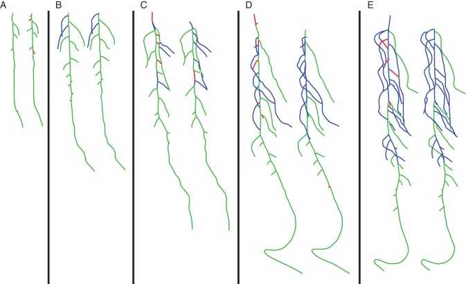
In addition to its interest as a quantitative evaluation tool that can be applied efficiently to a large data set, the proposed similarity indices have also been used to assess visually the main structural errors made by the evaluated reconstruction method. Figure 11 shows a sample of the tested root systems that exhibit this functionality: it highlights unmatched parts (i.e. the geometric errors, in red) and those that are inappropriately connected (i.e. the topological errors, in blue). This provides a useful tool that makes it possible to define an efficient methodology for the development of plant reconstruction methods.

Fig. 11.

Five examples of the comparison of automatic root system reconstruction (left) and their respective reference structures (right), highlighting geometrical errors in red and topological errors in blue. From left to right, the root systems are 7, 8, 10, 11, and 12 d old.

Conclusions

Our work addresses the problem of comparing automatic reconstruction methods of plant architecture from laser scanner data. For this purpose, a database of scans of reference structures produced by experienced researchers was constructed. Different methods from the literature were re-implemented in a common software framework and applied on the scan database. Our evaluation framework permits us to compare two structures by identifying their similar elements and by quantifying the similarity of their organization. A sensitivity analysis of the framework shows that it succeeds in capturing the variation of similarity between two structures. Its application to the different existing reconstruction methods of the literature makes it possible to set up a first comparative evaluation. While this study is more an example of comparison assessment than a definitive benchmarking, it still provides new insights into the different reconstruction methods.

In the future, a more complete evaluation will be carried out using a larger data set of scans and reference structures. In particular, it would be interesting to test the behaviour of the reconstruction methods on scans with various resolutions and/or coming from different environmental conditions to assess the sensitivity of the method to these factors.

This evaluation methodology is integrated in the OpenAlea platform and the databases will be made available to the research community. It will provide an opportunity for future reconstruction methods to quantify their improvement over previous methods. As a side product, this method and the scan database make it possible to train reconstruction methods by tuning their parameters for a given type of plant and scanning set-up. The parameters can then be re-used for reconstruction of similar scans. This tool is also particularly useful during the development of reconstruction methods by making it possible to assess improvements of regressions and rapidly to identify the errors visually.

LITERATURE CITED

- Alexa M, Behr J, Cohen-or D, Fleishman S, Levin D, Silva CT. Computing and rendering point set surfaces. IEEE Transactions on Visualization and Computer Graphics. 2003;9:3–15. [Google Scholar]
- Côté JF, Widlowski JL, Fournier RA, Verstraete MM. The structural and radiative consistency of three-dimensional tree reconstructions from terrestrial lidar. Remote Sensing of Environment. 2009;113:1067–1081. [Google Scholar]
- Diener J, Nacry P, Perin C, et al. An automated image-processing pipeline for high-throughput analysis of root architecture in OpenAlea. In: Sievänen R, Nikinmaa E, Godin C, Lintunen A, Nygren P, editors. Proceedings of the 7th International Workshop on Functional–Structural Plant Models. 2013. pp. 85–87. Saariselkä, Finland, 9–14 June 2013. [Google Scholar]
- Edmonds J, Karp RM. Theoretical improvements in algorithmic efficiency for network flow problems. Journal of the ACM. 1972;19:248–264. [Google Scholar]
- Ferraro P, Godin C. A distance measure between plant architectures. Annals of Forest Science. 2000;57:445–461. [Google Scholar]
- Godin C, Caraglio Y. A multiscale model of plant topological structures. Journal of Theoretical Biology. 1998;191:1–46. doi: 10.1006/jtbi.1997.0561. [DOI] [PubMed] [Google Scholar]
- Hu J, You S, Neumann U. Approaches to large-scale urban modeling. IEEE Computer Graphics and Applications. 2003;23:62–69. [Google Scholar]
- Livny Y, Yan F, Olson M, Chen B, Zhang H, El-Sana J. Automatic reconstruction of tree skeletal structures from point clouds. ACM Transaction on Graphics. 2010;29:151. [Google Scholar]
- Meijering E, Jacob M, Sarria JCF, Steiner P, Hirling H, Unser M. Design and validation of a tool for neurite tracing and analysis in fluorescence microscopy images. Cytometry Part A. 2004;58:167–176. doi: 10.1002/cyto.a.20022. [DOI] [PubMed] [Google Scholar]
- Pradal C, Boudon F, Nouguier C, Chopard J, Godin C. PlantGL: a Python-based geometric library for 3-D plant modelling at different scales. Graphical Models. 2009;71:1–21. [Google Scholar]
- Preuksakarn C, Boudon F, Ferraro P, Durand JB, Nikinmaa E, Godin C. Proceedings of the 6th International Workshop on Functional–Structural Plant Models. 2010. Reconstructing plant architecture from 3-D laser scanner data; pp. 16–18. [Google Scholar]
- Raumonen P, Kaasalainen M, Åkerblom M, et al. Fast automatic precision tree models from terrestrial laser scanner data. Remote Sensing. 2013;5:491–520. [Google Scholar]
- Runions A, Lane B, Prusinkiewicz P. Proceedings of Eurographics Workshop on Natural Phenomena 2007. 2007. Modeling trees with a space colonization algorithm; pp. 63–70. [Google Scholar]
- Sinoquet H, Rivet P, Godin C. Assessment of the three-dimensional architecture of walnut trees using digitising. Silva Fennica. 1997;31:265–273. [Google Scholar]
- Tarjan RE. CBMS-NFS Regional Conference Series in Applied Mathematics. 1983. Data structures and network algorithms. Society for Industrial and Applied Mathematics. [Google Scholar]
- Xu H, Gosset N, Chen B. Knowledge and heuristic-based modeling of laser-scanned trees. ACM Transactions on Graphics. 2007;26:19. [Google Scholar]
- Verroust A, Lazarus F. Extracting skeletal curves from 3d scattered data. Visual Computer. 2000;16:15–25. [Google Scholar]
- Yan D-M, Wintz J, Mourrain B, Wang W, Boudon F, Godin C. Proceedings of the 2009 11th IEEE International Conference on Computer-Aided Design and Computer Graphics. 2009. Efficient and robust reconstruction of botanical branching structure from laser scanned points; pp. 572–575. [Google Scholar]
- Zhang K, Jiang T. Some MAX SNP-hard results concerning unordered labeled trees. Information Processing Letters. 1994;49:249–254. [Google Scholar]