A plant cell division algorithm based on cell biomechanics and ellipse-fitting

Abstract

Background and Aims

The importance of cell division models in cellular pattern studies has been acknowledged since the 19th century. Most of the available models developed to date are limited to symmetric cell division with isotropic growth. Often, the actual growth of the cell wall is either not considered or is updated intermittently on a separate time scale to the mechanics. This study presents a generic algorithm that accounts for both symmetrically and asymmetrically dividing cells with isotropic and anisotropic growth. Actual growth of the cell wall is simulated simultaneously with the mechanics.

Methods

The cell is considered as a closed, thin-walled structure, maintained in tension by turgor pressure. The cell walls are represented as linear elastic elements that obey Hooke's law. Cell expansion is induced by turgor pressure acting on the yielding cell-wall material. A system of differential equations for the positions and velocities of the cell vertices as well as for the actual growth of the cell wall is established. Readiness to divide is determined based on cell size. An ellipse-fitting algorithm is used to determine the position and orientation of the dividing wall. The cell vertices, walls and cell connectivity are then updated and cell expansion resumes. Comparisons are made with experimental data from the literature.

Key Results

The generic plant cell division algorithm has been implemented successfully. It can handle both symmetrically and asymmetrically dividing cells coupled with isotropic and anisotropic growth modes. Development of the algorithm highlighted the importance of ellipse-fitting to produce randomness (biological variability) even in symmetrically dividing cells. Unlike previous models, a differential equation is formulated for the resting length of the cell wall to simulate actual biological growth and is solved simultaneously with the position and velocity of the vertices.

Conclusions

The algorithm presented can produce different tissues varying in topological and geometrical properties. This flexibility to produce different tissue types gives the model great potential for use in investigations of plant cell division and growth in silico.

INTRODUCTION

Cellular pattern studies and simulation of higher level processes such as phyllotaxis or vascular patterning call for models of the division and arrangement of cells into tissues (Smith et al., 2006; Merks et al., 2007). Many biophysiological processes in plant organs, such as gas transport, are strong functions of the microstructural geometry of the tissue (Ho et al., 2009, 2010, 2011, 2012), which is in turn dependent on cell division and the arrangement of cells.

In contrast to animal cells, plant cells have relatively rigid cell walls. The walls of the neighbouring cells are joined by the middle lamellas (Romberger et al., 1993). Walls of neighbouring cells do not slide with respect to each other. Therefore, cell topology is maintained except in the event of intercellular gas space formation or cell division. These aspects should be taken into account when considering cell division and expansive growth. The cell division rules proposed by Hofmeister (1863), Sachs (1878) and Errera (1886) remain the most prominent basis for modern thoughts on cell division. According to Hofmeister, the dividing wall is inserted at right angles to the axis of maximal growth, while Sachs suggested that the new wall intersects the side walls at right angles. Errera's rule states that the dividing wall should be the shortest one that partitions the mother cell into two equal daughter cells (reviewed by Prusinkiewicz and Runions, 2012).

Computer models of tissues with cell division based on position and orientation have been developed by Sahlin and Jönsson (2010). In their approach, the position of the new wall is determined to be either the centre of mass of the mother cell or a point inside the mother cell chosen randomly, while its orientation is chosen based on a number of criteria. Although this model includes cell growth mechanics and includes actual growth of the cell wall by changing the resting length of the cell wall, it does not limit the actual growth of the cell-wall resting length, and how turgor force is implemented does not allow for cell–cell interactions.

Besson and Dumais (2011) developed a rule for symmetric division of plant cells based on probabilistic selection of division planes. According to their work, Errera's rule of cell division failed to account for the variability observed in symmetric cell divisions, in particular that cells of identical shape do not necessarily adopt the same division plane. The variability in symmetric cell division is accounted for by introducing the concept of local minima rather than global minima. Robinson et al. (2011) introduced an asymmetric cell division algorithm in which the division wall is chosen as the shortest wall that passes through the nucleus of the mother cell. In their model, asymmetric cell division is achieved by displacing the nucleus of the mother cell from the centroid of the cell in a random direction.

The dynamic pattern of cell arrangement is not only a function of the position and orientation of division walls but also of the timing of cell division and growth of the tissue. The early work of Korn (1969) reintroduced by Merks and Glazier (2005) represents cells as a set of points, and growth is achieved by the addition of new points to a cell. Nakielski (2008) developed a model for growth and cell division based on the postulate of Hejnowicz (1984) that cells divide in relation to principal directions of growth (PDGs) and supported by the experimental work of Lintilhac and Vesecky (1981) and Lynch and Lintilhac (1997). PDGs are mutually perpendicular directions along which extreme growth rates are observed, which lead to unequal major and minor equivalent diameters for the cell. This is true for anisotropic growth, associated with anisotropic mechanical properties of the cell wall. They are in turn dependent on a growth tensor field defined at the organ level according to the work of Hejnowicz and Romberger (1984). Cell mechanics-based models for 2-D cell growth have been developed by several researchers (Dupuy et al., 2008, 2010; Sahlin and Jönsson, 2010; Gibson et al., 2011; Merks et al., 2011; Abera et al., 2013). The 2-D cell growth model developed by Abera et al. (2013) has recently been extended to a 3-D cell growth model (Abera et al., 2014).

Not all plant cells grow isotropically; anisotropic growth is also a common phenomenon. This anisotropy, defined as direction-dependent growth of a cell that leads to a mother cell with unequal major and minor diameters, is manifested as a consequence of anisotropic molecular wall structure, determined by differential spatial arrangement of the cellulose microfibrils that are generally organized in layers of parallel fibres (reviewed by Baskin, 2005; Schopfer, 2006). A different definition of anisotropy is the temporal and/or spatial difference in growth rate of the cell. For the latter, a cell can still be isotropic in shape (see Kwiatkowska and Dumais, 2003; Kwiatkowska, 2006). In the present paper, the first definition is used. Nakielski (2008) used this concept to incorporate overall tissue anisotropy in their model, which was based on PDGs. To our knowledge, although anisotropic growth of plant cells is a common phenomenon, the available literature on cell division models that use anisotropic cell growth is limited.

Based on the literature references detailed above, there is no single generic model. Some models are intended either for symmetric or for asymmetric cell division. Some are focused simply on the division rules, without incorporating the timing of cell division or the actual expansive growth and others do not consider cell mechanics when modelling cell growth. Most of the models introduced so far are based on isotropic growth. Hence, the objective of this paper is to develop a 2-D plant cell division algorithm that is generic in that it includes symmetric cell division by taking account of the randomness without abandoning Errera's rule of cell division. Furthermore, it accounts for asymmetric cell division, isotropic cell growth and anisotropic cell growth. It is based on cell growth mechanics, which accounts for cell–cell interaction through turgor force calculation and limits the resting length of the cell walls. In our model, because the cell division rules are based on ellipse-fitting, there is no need for an iterative procedure to find the position and orientation of the new dividing wall.

MATERIALS AND METHODS

Cell growth algorithm

In our model, the cell is considered a closed thin-walled structure, maintained in tension by turgor pressure. The cell walls of adjacent cells are modelled as parallel, linear elastic elements that obey Hooke's law, an approach similar to that used in other plant tissue models (Prusinkiewicz and Lindenmayer, 1990; Rudge and Haseloff, 2005; Dupuy et al., 2008, 2010; Gibson et al., 2011; Merks et al., 2011). Cell expansion then results from turgor pressure acting on the yielding cell-wall material. Growth is modelled by considering Newton's law. The following system of equations is solved for the velocity v and position x of the vertices i of the cell-wall network (only the main equation are presented here; futher details are given by Abera et al., 2013, 2014):

$${\mathit{m}}_i\frac{\text{d}{\mathbf{V}}_i}{\text{d}t}={\mathbf{F}}_{\mathrm{T},i}$$ (1)

$$\frac{\text{d}{\mathbf{X}}_i}{\text{d}t}={\mathbf{V}}_i$$ (2)

where m_i is the mass of the vertex, which is assumed to be unity, x_i (m) and v_i(m s^–1) are the position and velocity of vertex i, respectively, and F_T,i (N) is the total force acting upon this vertex. The resultant force on each vertex, the position of each vertex and thus the shape of the cells is computed as follows. The total force acting on a vertex is given by (Prusinkiewicz and Lindenmayer, 1990):

$${\mathbf{F}}_{\mathrm{T}}=\sum _{f\in F}{\mathbf{F}}_{\mathrm{turgor}}+\sum _{e\in E}{\mathbf{F}}_S+{\mathbf{F}}_{\mathrm{d}}$$ (3)

where F_turgor (N) are turgor forces on the set of cell faces F sharing the vertex, F_s (N) are tension forces from the set of edges (springs) sharing the vertex and

$${\mathbf{F}}_{\mathrm{d}}=-b\mathbf{v}$$ (4)

is a damping force, expressed as the product of a damping factor b (Ns m^–1) and the vertex velocity v. The damping force was included not only to capture the viscous nature of the matrix but also to give sufficient damping to avoid numerical oscillations in the solution. When the system is at equilibrium, the total force in eqn (3) is equal to zero.

From the calculation of cell expansion, cell growth is modelled by increasing the natural length of the springs associated with the growing cell, simulating biosynthesis of cell-wall material. At each time step the spring's extension from its resting length and the difference between the maximum attainable resting length of the spring and its current resting length, l_n, are used to compute the natural lengths of the springs as:

$$\frac{\mathrm{d}{l}_n}{\mathrm{d}t}=\frac{\text{1}}{\tau }(l-l_n)\left(\frac{l_{n,\max }-l_n}{l_{n,\max }}\right)$$ (5)

where l_n,max (m) is the maximum resting length of the spring above which the wall cannot expand irreversibly, and which is determined as a fixed percentage of the initial resting length, and τ is a time constant (s). In this way, resting length is coupled with force balance, allowing them to be solved together. In contrast to previous models (Rudge and Haseloff, 2005), there is thus no need to assume intermediate equilibrium to update the resting length of the cell wall.

To allow anisotropic expansion, which is a common mode of growth in plants (Baskin, 2005; Schopfer, 2006), the spring constant (k) and the maximum resting length (l_n,max) can be made to vary according to the orientation of the walls as follows:

$$k=k_{\min }+k_{\min }(C-\text{1})(\text{1}-\lambda )$$ (6)

$$l_{n,\max }=\lambda (C-\text{1})l_{n,0}+l_{n,0}$$ (7)

where k_min is the spring constant of walls aligned along the maximum growth direction, C is the ratio of the maximum resting length of the edges and the initial resting length of edges (l_n,max/l_n,0) and λ is a parameter defined between 0 and 1 according to the orientation of the edges as follows (Rudge and Haseloff, 2005):

$$\lambda =\text{1}-a{\text{sin}}^2\theta$$ (8)

where θ is the angle between the edges and the major axis of the cell and a is the degree of anisotropy defined on (0, 1). With a = 0 we get isotropic growth and with a = 1 we have anisotropic growth in the direction of the major axis of the cell. These equations allow us to switch growth from totally isotropic to any degree of anisotropy. All the parameters used in this model were taken from Abera et al. (2013).

Cell division algorithm

The moment in time when the cell divides was determined based on cell size. A dividing wall is inserted whenever a cell doubles its area. To determine the position and orientation of the new wall that divides the cell, an ellipse is fitted to the cell vertices (for details of the fitting algorithms, see Mebatsion et al., 2006, 2008). The outputs of the ellipse-fitting algorithm are the major and minor diameters (which are orthogonal to each other) and orientation (the direction of the major diameter) of the fitted ellipse. The new wall is then inserted along the shortest diameter of the fitted ellipse perpendicular to the longest diameter of the fitted ellipse (Fig. 1). Eventually, the mother cell, along with its entities (vertices, walls), is replaced by the two daughter cells. The cell vertices, walls and cell connectivity are then updated and cell expansion resumes. The division rules of the algorithm are based on the position and orientation of the dividing wall. The orientation the dividing wall is made to be along the minor diameter of the fitted ellipse normal to the major diameter (in accordance with both Errera's rule and Hofmeister's rule) whereas the position of the dividing wall can be made to vary to produce daughter cells with different sizes. For example, if the position is made to be at the centroid of the cell, the division will result in two similar daughter cells (geometrically symmetric cell division, which is in accordance with Errera's rule); otherwise it will result in two different daughter cells (geometrically asymmetric cell division). The position of the dividing wall in this case is moved to either direction along the major axis based on a random factor chosen from a uniform distribution between –0·8 and 0·8 (the range is chosen to avoid non-viable cells, which are very small if the range is between –1 and 1). There is also a good chance of symmetric cell division when the random factor is 0.

Fig. 1.

Illustration of the cell division algorithm. 2-D cell division is shown, where the blue lines are the boundaries of the mother cell, the green line is the fitted ellipse and the red line is the new wall dividing the two daughter cells.

Experimental data

The simulation data were compared with experimental data for shoot apical meristem (SAM) of Arabidopsis thaliana and leaf tissue of A. thaliana obtained from De Reuille et al. (2005) and De Veylder et al. (2001), respectively. We digitized the images to get individual cell coordinates using a Matlab program. The topological and geometrical property distributions are then calculated from the digitized coordinates. In De Reuille et al. (2005), their figure 5 shows how cell division in the SAM takes place by maintaining the same colour for the mother cell and the two daughter cells. The observation suggests the division is mostly symmetric. In De Veylder et al. (2001), their figure 7 provides a typical example of asymmetric cell division of meristematic leaf cells.

Fig. 5.

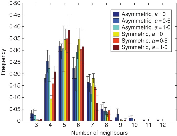
Distribution of the topology of cells. Values are means ± s.d. for five different simulations runs. Asymmetric and symmetric cell divisions are indicated in the key, with a = anisotropic value.

Fig. 7.

Cell area distribution. Cell area is normalized by the mean area of the cells in the tissue. Values are means ± s.d. for five different simulations runs. Asymmetric, asymmetric cell division; Symmetric, symmetric cell division; a, anisotropic value.

Geometric and topological properties

We have developed a program that calculates the geometric and topological properties of the cells for both the simulated tissues and the tissue from the confocal microscopy experimental data. The properties that we have considered were topology, cell shape (aspect ratio and interior angles) and cell size.

Topology

The topology of the cell aggregate (cell collection in a tissue) is defined in terms of the number neighbour cells that are in contact with a given cell. For both the simulated tissues and SAM from the experimental data, the algorithm calculates the number of cells that are in contact (neighbour cells) with a given cell and a frequency distribution of the number of cells was determined. The topology distributions of the tissues obtained from the model, using different cell division rules (geometrically similar daughter cells and geometrically different daughter cells together with the different anisotropic values), were compared statistically with each other and with that of the experimental tissue.

Cell shape

The cell shape distribution is characterized in this study by two distinct geometrical properties, namely aspect ratio and interior angle of the polygons representing the cell boundary.

The aspect ratio (a_r) of the cells was defined as:

$$a_r=\text{1 }-(l_1/l_2)$$ (9)

where l₁ and l₂ are the minor and major diameter of the fitted ellipse, respectively. With this definition, circular cells will have an aspect ratio of 0, whereas cells which have shapes far from circular will approach an aspect ratio of 1. The diameters of the equivalent ellipses were calculated according to the procedure outlined by Mebatsion et al. (2006).

The interior angles of the polygons, which represent cells in the virtual tissues generated with the different rules of cell division (symmetric and asymmetric) and growth modes (isotropic and anisotropic), were calculated. The distributions were then compared with each other. A comparison was also made with a distribution obtained by assuming that the cell polygons are regular (an ideal situation in which all interior angles of a polygon are assumed to be equal). The interior angles (i.e. at the vertices where two cell walls meet) were calculated using the inverse cosine function by defining two vectors starting from the common vertex heading away from it along the two walls of the cell sharing that vertex (Fig. 2). The interior angles for the regular polygons were calculated as:

(10)

where θ is interior angle and n is the number of sides of the polygon.

Fig. 2.

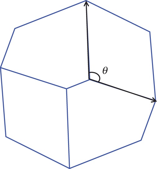
Illustration of the calculation of the interior angle. The procedure is repeated for each cell at each vertex.

Cell size

The size distribution of cell areas (2-D) was calculated. The areas of the cells were calculated by applying Green's theorem (Kreyszig, 2005).

Statistical comparison

Topological and geometrical (shape and size) properties of both microscopic cellular images and virtual cells were calculated and compared statistically. A two-sample Kolmogorov–Smirnov test was used to compare the distributions of these values. The null hypothesis was that both are from the same continuous distribution. The alternative hypothesis was that they were from different continuous distributions. The test statistic is the maximum height difference of the two data distributions on a cumulative distribution function. If the test statistic is greater than the critical value the null hypothesis is rejected. The P-value, which is dependent on the test statistics and the threshold with reference to the test significance, is normally used as criterion for whether to reject the null hypothesis. If the P-value is less than the test significance, the null hypothesis is rejected meaning that the two distributions are different. The result of the test was 1 if the test rejects the null hypothesis at a specified significance level, and 0 otherwise. We have used a 5 % significance level (Justel et al., 1997). The distributions were also compared by using the mean, standard deviation and skewness. The statistical comparision was done in Matlab (The Mathworks, Natick, MA, USA).

RESULTS

A demonstration of the cell division algorithm at different stages in time for symmetric cell division with isotropic growth is shown in Fig. 3. Several examples of tissues generated by the 2-D cell division algorithm are presented in Fig. 4. The tissues shown were generated using: (A) symmetric cell division with isotropic growth, (B) symmetric cell division with anisotropic growth value of 0·5, (C) symmetric cell division with anisotropic growth value of 1, (D) asymmetric cell division with isotropic growth, (E) asymmetric cell division with anisotropic growth value of 0·5 and (F) symmetric cell division with anisotropic growth value of 1. As can be seen from the figure, the algorithm can generate different kinds of tissues by employing different cell division rules and different cell growth modes. The visual differences between the tissues are evident from the figure. The topological and geometrical properties are analysed and discussed below. Five different simulation runs are used for each case. The number of cells used was 781, 350, 246, 474, 286 and 310 for symmetric cell division–isotropic growth, symmetric cell division–anisotropic growth (0·5), symmetric cell division–anisotropic growth (1), asymmetric cell division–isotropic growth, asymmetric cell division–anisotropic growth (0·5) and asymmetric cell division–anisotropic growth (1), respectively.

Fig. 3.

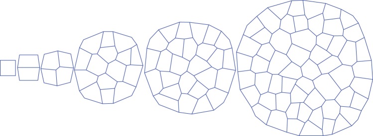
Illustration of the cell division algorithm at different stages in time.

Fig. 4.

Different virtual tissues obtained using: (A) symmetric cell division with isotropic growth; (B) symmetric cell division with anisotropic growth value of 0·5; (C) symmetric cell division with anisotropic growth value of 1; (D) asymmetric cell division with isotropic growth; (E) asymmetric cell division with anisotropic growth value of 0·5; and (F) asymmetric cell division with anisotropic growth value of 1. The red lines are new dividing walls separating the two daughter cells and the blue lines are old walls inherited from the mother cells.

Topology

The topological distribution, defined as the number of neighbour cells, showed a clear difference between the different tissues presented above. As can be seen from Fig. 5, there is a clear difference between tissues using the different cell division rules and growth modes, where the virtual tissues using symmetric cell division have a narrower distribution than those using asymmetric cell division rules (Table 1). Another interesting feature of these distributions is the skewness. Although all the cases presented here display skewness in the distribution of number of neighbours, the degree of skewness is lower for symmetric cell division (Table 1).

Table 1.

Standard deviation and skewness values of topology distribution

	Symmetric cell division		Asymmetric cell division
	s.d.	Skewness	s.d.	Skewness
Anisotropy = 0	0·99 ± 0·05	0·17 ± 0·23	1·42 ± 0·07	0·80 ± 0·27
Anisotropy = 0·5	1·10 ± 0·06	0·32 ± 0·19	1·45 ± 0·08	0·70 ± 0·34
Anisotropy = 1	0·95 ± 0·05	0·23 ± 0·52	1·14 ± 0·14	0·28 ± 0·18

Values are means for the five different runs for each case with ± values indicating the standard deviation in each case.

The different cell divisions are also tested on how well they fit to Lewis' law, which states that a linear relationship exists between the number of neighbours and the area of cells (Lewis, 1928). The results are presented in Fig. 6. The error bars indicate the standard deviation of the mean normalized cell area. The linear relationship between the mean normalized cell area and the number of neighbours is respected more in the symmetric cell division rules than their asymmetric counterparts (see the affine fit of the data drawn in blue in Fig. 6 and Table 2). The norm of the residuals is normalized by the size of the data used in the fitting to get a fair comparison. The symmetric cell division rules have a lower norm of residuals than their asymmetric counterparts, suggesting a better linear fit. The asymmetric cell division rules demonstrated higher standard deviations whereas the symmetric cell division rules showed a lower slope than that given by Lewis' law. These results are in agreement with those of Sahlin and Jönsson (2010). The symmetric cell division algorithm with isotropic growth, in which only the peripheral cells were allowed to divide, matched perfectly with Lewis' law.

Fig. 6.

The relationship between number of neighbours and cell area: (A) symmetric cell division with isotropic growth; (B) asymmetric cell division with isotropic growth; (C) symmetric cell division with anisotropic growth value of 0·5; (D) asymmetric cell division with anisotropic growth value of 0·5; (E) symmetric cell division with anisotropic growth value of 1; (F) asymmetric cell division with anisotropic growth value of 1; (G) symmetric cell division with isotropic growth where cell division is restricted to the boundary cells; and (H) experimental data of Arabidopsis shoot apical meristem (SAM). Sym, symmetric; Asym, asymmetric; Symp, symmetric peripheral cells. Lewis' law equation, A_n = (n – 2)/4, is shown in red, where A_n is the mean normalized cell area and n is number of neighbours. The blue lines represent the affine fit of the data. Cell area is normalized by dividing the individual cell area by the mean of the cell areas in the tissue.

Table 2.

Norm of residuals (normalized by size of the data) of a linear fit to the relationship between topology and mean normalized cell area for the different simulation cases

Sym, a = 0	Sym, a = 0·5	Sym, a = 1	Asym, a = 0	Asym, a = 0·5	Asym, a = 1	Symp	SAM
0·2121	0·1902	0·1896	0·5209	0·4762	0·4665	0·3232	0·2626

Sym, symmetric; Asym, asymmetric; Symp, symmetric peripheral cells; SAM, shoot apical meristem; a, anisotropic value.

Cell size distribution

The cell size distribution, presented here as the distribution of mean normalized cell area, is an important geometrical property used to compare the performance of different cell division rules. As can be seen from Fig. 7, the cell size distribution shows a clear distinction between the various division rules investigated. In particular, the difference between the symmetric cell division and asymmetric cell division is remarkable. Besides the difference between the spread of the distribution, which is evident from Fig. 7, the degree of skewness is another important difference between the different division rules employed (Table 3). The spread of the distributions as well as the degree of skewness are more pronounced in the asymmetric cell division than the corresponding symmetric cell division, similar to what was found for the cell topology.

Table 3.

Standard deviation and skewness values of cell area distribution

	Symmetric cell division		Asymmetric cell division
	s.d.	Skewness	s.d.	Skewness
Anisotropy = 0	0·36 ± 0·03	1·00 ± 0·20	0·76 ± 0·07	1·70 ± 0·67
Anisotropy = 0·5	0·33 ± 0·05	1·18 ± 0·41	0·67 ± 0·08	0·64 ± 0·32
Anisotropy = 1	0·30 ± 0·03	1·30 ± 0·69	0·55 ± 0·05	0·22 ± 0·22

Values are means for the five different runs for each case with ± values indicating the standard deviation in each case.

Cell shape distribution

Cell shape distribution is analysed here by means of two geometrical properties, namely aspect ratio and the internal angle of the polygons representing the cell boundary (see Methods).

Aspect ratio distribution

The cell aspect ratio distributions of the tissues obtained using different cell division rules and growth modes are presented in Fig. 8 and Table 4. As can be seen from the figure and table, the mean aspect ratio values of the corresponding symmetric and asymmetric cell division rules immediately after cell division (before expansion) are almost equal. Their difference is reflected in the spread of the distribution, as shown by the corresponding standard deviation values. The symmetric cell division generally produces a narrower distribution than the asymmetric cell division. The difference in the skewness of the distribution is apparent: the asymmetric cell division rules result in a higher positive degree of skewness as opposed to little or no skewness for their symmetric counterparts. Among the cell growth types investigated, isotropic cell growth has lower aspect ratio values than anisotropic cell growth, although this difference is reduced after cell division. The effect of the growth type used is mainly manifested in the overall tissue shape (see Fig. 4).

Fig. 8.

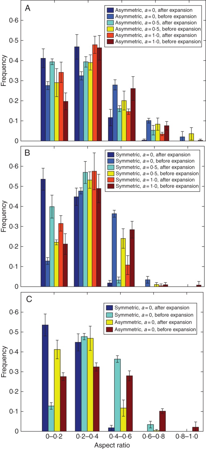
Aspect ratio distributions of cells: (A) asymmetric cell division with different degrees of anisotropy; (B) symmetric cell division with different degrees of anisotropy; and (C) a comparison between symmetric and asymmetric cell divisions. Values are means ± s.d. for five different simulations runs. Asymmetric, asymmetric cell division; Symmetric, symmetric cell division; a, anisotropic value.

Table 4.

Mean, standard deviation and skewness values of aspect ratio distribution

		Anisotropy = 0		Anisotropy = 0·5		Anisotropy = 1
		Expanded	Not expanded	Expanded	Not expanded	Expanded	Not expanded
Symmetric cell division	Mean	0·2 ± 0·001	0·36 ± 0·001	0·23 ± 0·01	0·32 ± 0·01	0·26 ± 0·01	0·32 ± 0·02
	s.d.	0·09 ± 0·002	0·13 ± 0·01	0·10 ± 0·01	0·13 ± 0·01	0·12 ± 0·02	0·14 ± 0·02
	Skewness	0·31 ± 0·11	−0·04 ± 0·10	0·10 ± 0·30	−0·05 ± 0·13	0·09 ± 0·27	0·13 ± 0·38
Asymmetric cell division	Mean	0·24 ± 0·01	0·36 ± 0·02	0·27 ± 0·01	0·33 ± 0·03	0·27 ± 0·01	0·34 ± 0·01
	s.d.	0·13 ± 0·01	0·20 ± 0·02	0·16 ± 0·01	0·20 ± 0·02	0·15 ± 0·004	0·16 ± 0·004
	Skewness	0·56 ± 0·19	0·40 ± 0·14	0·80 ± 0·11	0·71 ± 0·20	0·69 ± 0·15	0·33 ± 0·13

Values are means for the five different runs for each case with ± values indicating the standard deviation in each case.

Interior angle

The interior angles of the polygons representing the cell are calculated just after cell division and after expansive growth, when the cells have achieved equilibrium. These distributions are compared with each other and with the interior angle distribution obtained assuming all the polygons are regular (an ideal situation in which all interior angles of a polygon representing a cell are assumed to be equal). As most of the cells have six sides, symmetric cell division converges to 120°, better than its asymmetric counterparts (Fig. 9). Although their mean values are more or less equal, there is a clear difference in the width of the distribution as represented by its standard deviation (Table 5). The ideal internal angle distributions of the different cell division rules employed are narrower than their respective actual distributions. The interior angle distributions of the tissues obtained after cell expansion better approximate the respective ideal interior angle distributions in terms of both the standard deviation and the skewness of the distributions (Table 5). In both the aspect ratio distribution and the interior angle distribution, the distributions after cell expansion approximate the ideal distributions better than those just after cell division.

Fig. 9.

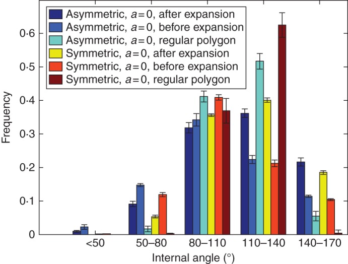
Interior angle distribution comparison of symmetric and asymmetric cell divisions. Values are means ± s.d. for five different simulations runs. Asymmetric, asymmetric cell division; Symmetric, symmetric cell division; a, anisotropic value.

Table 5.

Mean, standard deviation and skewness values of internal angle distribution

	Symmetric cell division			Asymmetric cell division
	Mean	s.d.	Skewness	Mean	s.d.	Skewness
Expanded	116·8 ± 0·26	23·4 ± 0·47	0·12 ± 0·03	115·8 ± 0·20	27·0 ± 0·72	–0·211 ± 0·06
Not expanded	116·8 ± 0·26	35·6 ± 0·07	0·56 ± 0·018	115·8 ± 0·20	38·0 ± 0·54	0·28 ± 0·08
Regular polygon	116·8 ± 0·26	11·2 ± 0·47	–0·83 ± 0·30	115·8 ± 0·20	16·1 ± 0·87	–0·74 ± 0·17

Values are means for the five different runs for each case with ± values indicating the standard deviation in each case.

Comparison of real and virtual topological and geometrical properties

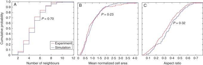
As demonstrated by Besson and Dumais (2011) and Prusinkiewicz (2011), seeking an exact prediction of a cell division pattern is as futile as attempting to predict the exact sequence of numbers produced by repetitively throwing a die. Only the statistical characteristics of these processes, as opposed to individual outcomes, can be meaningfully anticipated. In this regard, the visual, topological and geometrical comparisons of the different cell division rules with experimental data are presented here. The image with 347 cells obtained from a confocal microscopy was taken from De Reuille et al. (2005) and digitized by a Matlab code (Fig. 10A). Comparison of the cell area distribution, topology distribution and aspect ratio distribution (Fig. 11) suggests that symmetric cell division with isotropic growth has superior visual, topological and geometrical similarity to the experimental data than the other division rules investigated (Table 6). The experimental data as well as symmetric cell division, where cell division is restricted to the peripheral cells, were well fitted to Lewis' law (see Fig. 6G, H). Two-sample Kolmogorov–Smirnov tests were made between the best performing division rule (symmetric cell division with isotropic growth) and the experimental data (Fig. 12 and Table 6). The comparisons are made at 5 % significance level (see Methods). The results suggest the distributions are not significantly different. The different simulation cases were also compared with a meristematic leaf tissue image obtained from De Veylder et al. (2001) and digitized with a Matlab code (see Fig. 10B). The image contains 253 cells. Comparison of the cell area distribution, topology distribution and aspect ratio distribution (Fig. 13 and Table 6) suggest that asymmetric cell division generally shows superior topological and geometrical similarity to the experimental data than their symmetric counterparts. Two-sample Kolmogorov–Smirnov tests made between the data obtained using asymmetric cell division with isotropic growth and the experimental data obtained from De Veylder et al. (2001) showed the results are not significantly different. The results of the comparison are presented in Fig. 14.

Fig. 10.

Digitized shoot apical meristem of Arabidopsis thaliana taken from De Reuille et al. (2005) where cell division is mainly symmetric (A) and digitized meristematic leaf cells taken from De Veylder et al. (2001) where cell division is mainly asymmetric (B).

Fig. 11.

Geometrical and topological property comparisons of virtual tissues generated by the algorithm and a tissue obtained experimentally: (A) cell area distribution; (B) topology distribution; and (C) aspect ratio distribution. Asym, asymmetric cell division; Sym, symmetric cell division; SAM, shoot apical meristem; a, degree of anisotropy. Density in these plots represents frequency density.

Table 6.

P-values (expressed as a percentage) of the comparisons of the experimental data with the data obtained by the different simulation cases

		Symmetric cell division			Asymmetric cell division
		a = 0	a = 0·5	a = 1	a = 0	a = 0·5	a = 1
Cell area	SAM	21	7	4·5	4×10–12	7 × 10–6	9 × 10–6
	Meristematic leaf	8 × 10–7	8 × 10–6	1 × 10–6	23	11·6	32
Topology	SAM	94	24	2·9 × 10–2	0·27	9 × 10–4	0·3
	Meristematic leaf	5 × 10–26	9 × 10–14	1 × 10–7	70	28	2 × 10–4
Aspect ratio	SAM	40	38	46	33	4	93
	Meristematic leaf	2 × 10–2	13	19	32	51	89

The comparison is done using a two-sample Kolmogorov–Smirnov test. SAM, shoot apical meristem; a, anisotropic value.

Fig. 12.

Statistical comparison of geometrical and topological properties of virtual tissues generated by the algorithm using symmetric cell division with isotropic growth and a shoot apical meristem obtained from experiment using a two-sample Kolmogorov–Smirnov test.

Fig. 13.

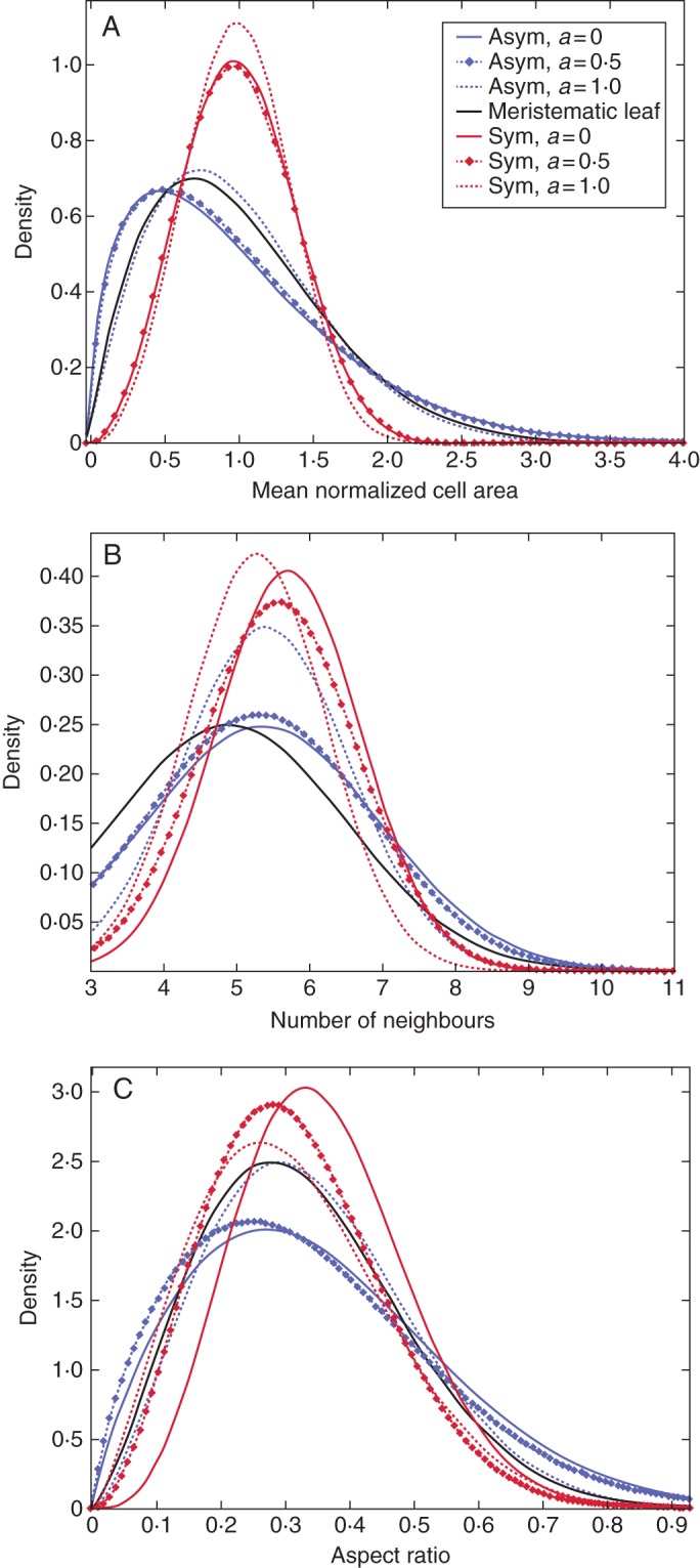
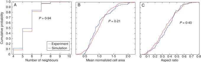
Geometrical and topological property comparisons of virtual tissues generated by the algorithm using asymmetric cell division with isotropic growth and a real meristematic leaf tissue obtained experimentally (from De Veylder et al., 2001): (A) cell area distribution; (B) topology distribution; and (C) aspect ratio distribution. Asym, asymmetric cell division; Sym, symmetric cell division; a, degree of anisotropy. Density in these plots represents frequency density.

Fig. 14.

Statistical comparison of geometrical and topological properties of virtual tissues generated by the algorithm using asymmetric cell division and a meristematic leaf tissue obtained experimentally using a two-sample Kolmogorov–Smirnov test.

DISCUSSION

We have developed a generic cell division algorithm based on cell-wall mechanics that is capable of producing different tissues varying both in geometrical and in topological property distributions of the cells as well as in the overall shape of the tissues. The algorithm provides a robust cell division model based on ellipse-fitting to find the position and orientation of the dividing wall and incorporates cell-wall mechanics for growth. Using the developed algorithm, we have generated different tissues. We have studied tissues which were generated using cell division rules of equally sized daughter cells and unequally sized daughter cells. Isotropic or anisotropic growth modes were used for each case. We have analysed the topologies and geometries of simulated tissues and compared them with experimental data to test the performance of different division rules (symmetric and asymmetric in a geometric sense). A comparison is also made among the virtual tissues generated using the different cell division and growth types (isotropic, anisotropic). We have also investigated how well tissues fitted to Lewis' law, which states that a linear relationship exists between the number of neighbours and the area of cells (Lewis, 1928).

Alim et al. (2012) investigated the effect cell division orientation on tissue growth heterogeneity. Cell growth in their approach was implemented by minimizing the difference between the second area moment of a target ellipse (which grows with time) and that of the cell calculated from its vertices. They found that tissue heterogeneity is more pronounced where cell division with randomly orientated division walls is used. Our result also allows the same conclusion.

The role of mechanics on cell expansion was detailed by Abera et al. (2013, 2014, and references therein), where a cell is represented as a thin-walled structure maintained in tension by turgor pressure. The cells will respond by increasing the resting length of the cell walls (simulating actual growth) to alleviate the mechanical stress induced by the tension. The role of mechanical stress on the orientation of the dividing wall has been explained by different authors (e.g. Lynch and Lintilhac, 1997; Lintilhac and Vesecky, 1981; Hejnowicz and Romberger, 1984). Nakielski (2008) developed a model based on these studies for root growth. These are studies based on the idea of growth tensors (GTs), which lead to mutually orthogonal PDGs. In their work (Hejnowicz and Romberger, 1984; Nakielski, 2008), they first define organ shape-based GTs, which help to define the velocities of the vertices of the cell mesh and the cell area increases as the vertices move governed by the GT field defined on the organ level. When a cell is ready to divide, the PDGs that are predefined by the GT based on the location of the cell with regard to the GT will be used to determine the orientation of the dividing wall. The diameters of the mother cell along the PDGs will be calculated and the dividing wall is inserted along the shorter of these diameters.

In our approach, the growth biomechanics govern the shape of the mother cell on which an ellipse is fitted to decide how the cell should divide. PDGs are mutually perpendicular diameters that can be obtained if you fit an equivalent ellipse to the vertices of the cell (minor and major diameters of the ellipse). Therefore, regarding the way the cell division wall orientation is determined, the two approaches should lead to a similar result (see Alim et al., 2012). The most important difference between their approach and ours is in their approach the PDGs are predefined based on location (because the GTs are predefined at organ level) whereas in our approach it is the mechanics that leads to the shape of the mother cell based on which it divides. Note that in cases where growth is started from an already elongated cell and maximum growth rate is along the shorter diameter, the two approaches will lead to different orientation for the dividing wall. In this case, when using the ellipse-fitting algorithm, the orientation of the dividing wall should be along the orientation of the major diameter of the fitted ellipse.

The algorithm can produce the variability observed in symmetric cell division. Besson and Dumais (2011) achieved the variability observed in symmetric cell division by introducing the concept of local minima instead of the global minima of Errera's rule for selection of the dividing wall. In our model, this was achieved without abandoning the founding rule of cell division suggested by Errera (1886). An ellipse-fitting procedure was used to determine the position and orientation of the dividing wall. The minor diameter of the ellipse through the centroid was used as the position and orientation of the dividing wall. If the fitted ellipse is a circle, we have infinitely many possible orientations for the candidate dividing wall. The random selection of one of them made it possible to produce the variability observed in symmetric cell division (see Fig. 4A). Ellipse-fitting has been used in previous studies (e.g. Gibson et al., 2011; Merks et al., 2011) to determine the position of the new dividing wall, but its importance to produce randomness even in symmetric cell division has not been put forward. This randomness is an important property that represents biological variability observed in nature.

Robinson et al. (2011) demonstrated asymmetric cell division in the leaves of arabidopsis, where the nucleus is displaced from the geometrical centre of the cell by cell polarity switching. In our model, asymmetric cell division is achieved by random displacement of the dividing wall along the major diameter of the fitted ellipse. This random displacement of the dividing wall is the equivalent of displacement of the nucleus from the geometrical centre of the cell, which could lead to two daughter cells that are different in size as well as in topology (see Fig. 4D–F). Our model has the added advantage that it incorporates cell mechanics in the growth model. By making the mechanical properties and maximum resting length of the walls dependent on direction, the model allows both isotropic and anisotropic cell growth, which leads to different simulated tissues (see Fig. 4). Although most of the meristematic cells that are undifferentiated obey symmetric cell division with isotropic growth, asymmetric cell division and anisotropic growth also have great potential to account for differentiation of meristem tissue into different specialized tissues.

Gibson et al. (2011) used the same cell representation as we do here. They developed differential equations and Newton's law was used to solve force balance on the vertices. In contrast to their model, ours assigns spring constant values, which are inversely proportional to wall length, whereas in their model the same spring constant value, independent of length, is assumed. Moreover, their model did not simulate actual growth of the cell walls; rather, they used a constant resting length throughout the simulation. They studied only isotropic mechanical properties of the cell wall. Therefore, our model provides a better representation of the cell mechanics and actual growth of the cell wall, which actually mimics the biosynthesis of cell-wall materials.

Merks et al. (2011) introduced a cell-based computer modelling framework, ‘VirtualLeaf’, for plant tissue morphogenesis. They used a Monte Carlo-based energy minimization algorithm. The energy of the system was calculated from cell area-related turgor pressure force and the tension force of the walls. They used the same cell representation as we do here. In contrast to their probabilistic determination of position of vertices, ours uses a deterministic approach based on Newton's law of force balances. In addition, they insert a new node to simulate cell-wall yielding after length exceeded four times its initial value while ours actually simulates growth of the resting length of the walls using differential equations simultaneously with mechanics. While their model presents a simplified software platform, ours offers better representation of the actual growth of the cell wall.

The cell division algorithms can be coupled to 2-D expansive plant cell growth models (Abera et al., 2013), where the initial topology was, for example, obtained from a 2-D Voronoi tessellation. The cell division algorithm has more biological justification than the Voronoi tessellations, which were initiated from random generating points, which is simply a partition of a given area cell topology into a number of regions, representing the individual cells.

In particular cases where the dividing wall is not a function of the shape of the mother cell, such as those observed in periclinal and anticlinal cell divisions (Howell, 1998; Evert, 2006), special care should be taken in using the ellipse-fitting algorithm. Periclinal (division walls parallel to the surface): this usually leads to relatively large new wall as the mother cells are elongated cells along the periphery. In this case, the ellipse-fitting can still be used to determine the position and orientation of the new wall but the major diameter instead of the minor diameter of the ellipse has to be used. Anticlinal (division walls at right angles to the surface): this usually leads to short new wall and the ellipse-fitting can still be used although caution has to be taken when the fitted ellipse is a circle, where there are infinitely many candidate short walls, to ensure the chosen short wall is the one that is normal to the surface.

CONCLUSIONS

The cell division algorithm developed here can produce tissues that have different topological and geometrical properties. This flexibility to produce different tissue types gives the model great potential for use in in silico investigations of plant cell division and growth. The cell division algorithms take account of both cell shape and topology. The model is based on cell mechanics, where the cell wall mechanical properties, fluid matrix inside the cell and cell turgor pressure are taken into account. The equations for actual growth of the cell walls (change in resting length of the walls) and cell division are solved continuously. It is generic in that a switch between isotropic growth and anisotropic growth as well as between symmetric cell division and asymmetric cell division is automatic and easy, which makes the model convenient to adapt to a specific case study. Finally, the model is robust as there is no need for an iterative procedure to find the shortest wall for cell division. In our algorithm, the division wall is inserted along the orientation of the minor diameter of the fitted ellipse. The geometrical properties of the simulated tissues were compared with experimental data for SAM. Symmetric cell division with isotropic growth best fits the experimental data.

LITERATURE CITED

- Abera MK, Fanta SW, Verboven P, Ho QT, Carmeliet J, Nicolai BM. Virtual fruit tissue generation based on cell growth modeling. Journal of Food and Bioprocess Technology. 2013;6:859–869. [Google Scholar]
- Abera MK, Verboven P, Herremans E, et al. 3D virtual pome fruit tissue generation based on cell growth modeling. Journal of Food and Bioprocess Technology. 2014;7:542–555. [Google Scholar]
- Alim K, Hamant O, Boudaoud A. Regulatory role of cell division rules on tissue growth heterogeneity. Frontiers in Plant Science. 2012;3:174. doi: 10.3389/fpls.2012.00174. [DOI] [PMC free article] [PubMed] [Google Scholar]
- Baskin TI. Anisotropic expansion of the plant cell wall. Annual Review of Cellular Developmental Biology. 2005;21:203–222. doi: 10.1146/annurev.cellbio.20.082503.103053. [DOI] [PubMed] [Google Scholar]
- Besson S, Dumais J. A universal rule for the symmetric division of plant cells; Proceedings of the National Academy of Sciences of the United States of America; 2011. pp. 6294–6299. [DOI] [PMC free article] [PubMed] [Google Scholar]
- De Reuille PB, Bohn-Courseau I, Godin C, Traas J. A protocol to analyse cellular dynamics during plant development. Plant Journal. 2005;44:1045–1053. doi: 10.1111/j.1365-313X.2005.02576.x. [DOI] [PubMed] [Google Scholar]
- De Veylder L, Beeckman T, Beemster GTS, et al. Functional analysis of cyclin-dependent kinase inhibitors of arabidopsis. Plant Cell. 2001;13:1653–1667. doi: 10.1105/TPC.010087. [DOI] [PMC free article] [PubMed] [Google Scholar]
- Dupuy L, Mackenzie J, Rudge T, Haseloff J. A system for modelling cell–cell interactions during plant morphogenesis. Annals of Botany. 2008;101:1255–1265. doi: 10.1093/aob/mcm235. [DOI] [PMC free article] [PubMed] [Google Scholar]
- Dupuy L, Mackenzie J, Haseloff J. Coordination of plant cell division and expansion in a simple morphogenetic system; Proceedings of the National Academy of Sciences of the United States of America; 2010. pp. 2711–2716. [DOI] [PMC free article] [PubMed] [Google Scholar]
- Errera L. Sur une condition fondamentale d'équilibre des cellules vivantes. Comptes Rendus Hebdomadaires des Séances de l'Académie des Sciences. 1886;103:822–824. [Google Scholar]
- Evert RF. Essu's plant anatomy: meristems, cells, and tissues of the plant body, their structure, function and development. 3rd edn. New York: Wiley; 2006. [Google Scholar]
- Gibson WT, Veldhuis JH, Rubinstein B, et al. Control of the mitotic cleavage plane by local epithelial topology. Cell. 2011;144:427–438. doi: 10.1016/j.cell.2010.12.035. [DOI] [PMC free article] [PubMed] [Google Scholar]
- Hejnowicz Z. Trajectories of principal growth directions. Natural coordinate system in plant growth. Acta Societatis Botanicorum Poloniae. 1984;53:29–42. [Google Scholar]
- Hejnowicz Z, Romberger JA. Growth tensor of plant organs. Journal of Theoretical Biology. 1984;110:93–114. [Google Scholar]
- Ho Q, Verboven P, Mebatsion H, Verlinden B, Vandewalle S, Nicolai B. Microscale mechanisms of gas exchange in fruit tissue. New Phytologist. 2009;182:163–174. doi: 10.1111/j.1469-8137.2008.02732.x. [DOI] [PubMed] [Google Scholar]
- Ho Q, Verboven P, Verlinden B, et al. Genotype effects on internal gas gradients in apple fruit. Journal of Experimental Botany. 2010;61:2745–2755. doi: 10.1093/jxb/erq108. [DOI] [PubMed] [Google Scholar]
- Ho Q, Verboven P, Verlinden B, et al. A 3-D multiscale model for gas exchange in fruit. Plant Physiology. 2011;155:1158–1168. doi: 10.1104/pp.110.169391. [DOI] [PMC free article] [PubMed] [Google Scholar]
- Ho Q, Verboven P, Yin X, Struik P, Nicolai B. A microscale model for combined CO2 diffusion and photosynthesis in leaves. PLOS ONE. 2012;7:e48376. doi: 10.1371/journal.pone.0048376. [DOI] [PMC free article] [PubMed] [Google Scholar]
- Hofmeister W. Zusatze und berichtigungen zu den 1851 veröffentlichen untersuchungen der entwicklung höherer kryptogamen. Jahrbucher für Wissenschaft und Botanik. 1863;3:259–293. [Google Scholar]
- Howell SH. Molecular genetics of plant development. Cambridge: Cambridge University Press; 1998. [Google Scholar]
- Justel A, Pena D, Zamar R. A multivariant Kolmogorov–Smirnov test of goodness of fit. Statistics and Probability Letters. 1997;35:251–259. [Google Scholar]
- Korn RW. A stochastic approach to the development of Coleocheate. Journal of Theoretical Biology. 1969;24:147–158. doi: 10.1016/s0022-5193(69)80042-1. [DOI] [PubMed] [Google Scholar]
- Kreyszig E. Advanced engineering mathematics. New York: Wiley; 2005. [Google Scholar]
- Kwiatkowska D. Flower primordium formation at the Arabidopsis shoot apex: quantitative analysis of surface geometry and growth. Journal of Experimental Botany. 2006;57:571–580. doi: 10.1093/jxb/erj042. [DOI] [PubMed] [Google Scholar]
- Kwiatkowska D, Dumais J. Growth and morphogenesis at the vegetative shoot apex of Anagallis arvensis L. Journal of Experimental Botany. 2003;54:1585–1595. doi: 10.1093/jxb/erg166. [DOI] [PubMed] [Google Scholar]
- Lewis FT. The correlation between cell division and the shapes and sizes of prismatic cells in the epidermis of Cucumis. Anatomical Records. 1928;38:341–376. [Google Scholar]
- Lintilhac PM, Vesecky TB. Mechanical stress and cell wall orientation in plants. II. The application of controlled directional stress to growing plants; with a discussion on the nature of the wound reaction. American Journal of Botany. 1981;68:1222–1230. [Google Scholar]
- Lynch TM, Lintihlac PM. Mechanical signals in plant development: a new method for single cell studies. Developmental Biology. 1997;191:246–256. doi: 10.1006/dbio.1996.8462. [DOI] [PubMed] [Google Scholar]
- Mebatsion HK, Verboven P, Ho QT, et al. Modelling fruit microstructure using novel ellipse essellation algorithm. CMES – Computer Modeling in Engineering and Sciences. 2006;14:1–14. [Google Scholar]
- Mebatsion H, Verboven P, Jancsók P, Ho Q, Verlinden B, Nicolai B. Modelling 3D fruit tissue microstructure using a novel ellipsoid tessellation algorithm. CMES – Computer Modeling in Engineering and Sciences. 2008;29:137–149. [Google Scholar]
- Merks RMH, Glazier JA. A cell-centered approach to developmental biology. Physica A. 2005;352:113–130. [Google Scholar]
- Merks RMH, Van de Peer Y, Inzé D, Beemster GTS. Canalization without flux sensors: a traveling-wave hypothesis. Trends in Plant Science. 2007;12:384–390. doi: 10.1016/j.tplants.2007.08.004. [DOI] [PubMed] [Google Scholar]
- Merks RMH, Guravage M, Inzé D, Beemster GTS. Virtualleaf: an open-source framework for cell-based modeling of plant tissue growth and development. Plant Physiology. 2011;155:656–666. doi: 10.1104/pp.110.167619. [DOI] [PMC free article] [PubMed] [Google Scholar]
- Nakielski J. The tensor-based model for growth and cell divisions of the root apex. I. The signicance of principal directions. Planta. 2008;228:179–189. doi: 10.1007/s00425-008-0728-y. [DOI] [PubMed] [Google Scholar]
- Prusinkiewicz P. Inherent randomness of cell division patterns; Proceedings of the National Academy of Sciences of the USA; 2011. pp. 5933–5934. [DOI] [PMC free article] [PubMed] [Google Scholar]
- Prusinkiewicz P, Lindenmayer A. The algorithmic beauty of plants. New York: Springer; 1990. [Google Scholar]
- Prusinkiewicz P, Runions A. Computational models of plant development and form. New Phytologist. 2012;193:549–569. doi: 10.1111/j.1469-8137.2011.04009.x. [DOI] [PubMed] [Google Scholar]
- Robinson S, Barbier de Reuille P, Chan J, Bergmann D, Prusinkiewicz P, Coen E. Generation of spatial patterns through cell polarity switching. Science. 2011;333:1436–1440. doi: 10.1126/science.1202185. [DOI] [PMC free article] [PubMed] [Google Scholar]
- Romberger JA, Hejnowicz Z, Hill JF. Plant structure: function and development. Berlin: Springer; 1993. [Google Scholar]
- Rudge T, Haseloff J. A computational model of cellular morphogenesis in plants. Lecture Notes in Computer Science: Advances in Artificial Life. 2005;3630:78–87. [Google Scholar]
- Sachs J. Über die anordnung der zellen in jüngsten pflanzentheilen. Arbeiten des Botanischen Instituts in Würzburg. 1878;2:46–104. [Google Scholar]
- Sahlin P, Jönsson H. A modeling study on how cell division affects properties of epithelial tissues under isotropic growth. PLOS ONE. 2010;5:e11750. doi: 10.1371/journal.pone.0011750. [DOI] [PMC free article] [PubMed] [Google Scholar]
- Schopfer P. Biomechanics of plant growth. American Journal of Botany. 2006;93:1415–1425. doi: 10.3732/ajb.93.10.1415. [DOI] [PubMed] [Google Scholar]
- Smith RS, Guyomarc'h S, Mandel T, Reinhardt D, Kuhlemeier C, Prusinkiewicz P. A plausible model of phyllotaxis. Proceedings of the National Academy of Sciences of the United States of America. 2006;103:1301–1306. doi: 10.1073/pnas.0510457103. [DOI] [PMC free article] [PubMed] [Google Scholar]