Interaction of a screw dislocation with a nano-sized, arbitrarily shaped inhomogeneity with interface stresses under anti-plane deformations

Abstract

We propose an elegant and concise general method for the solution of a problem involving the interaction of a screw dislocation and a nano-sized, arbitrarily shaped, elastic inhomogeneity in which the contribution of interface/surface elasticity is incorporated using a version of the Gurtin–Murdoch model. The analytic function inside the arbitrarily shaped inhomogeneity is represented in the form of a Faber series. The real periodic function arising from the contribution of the surface mechanics is then expanded as a Fourier series. The resulting system of linear algebraic equations is solved through the use of simple matrix algebra. When the elastic inhomogeneity represents a hole, our solution method simplifies considerably. Furthermore, we undertake an analytical investigation of the challenging problem of a screw dislocation interacting with two closely spaced nano-sized holes of arbitrary shape in the presence of surface stresses. Our solutions quite clearly demonstrate that the induced elastic fields and image force acting on the dislocation are indeed size-dependent.

1. Introduction

The elastic interaction between dislocations and fibres (often represented as elastic inhomogeneities) is a classical topic in micromechanics [1]. When the diameters of the fibres are in the nanoscale range (e.g. less than 100 nm), surface/interface stresses, surface tension and surface energies become significant when formulating and analysing the corresponding interaction problem [2,3].

One of the most celebrated models of surface/interface elasticity is the Gurtin–Murdoch surface model, originally proposed by Gurtin, Murdoch and co-workers [4,5] and most recently elucidated by Ru [6]. Many size-dependent phenomena present at the nanoscale have been explained by incorporating the Gurtin–Murdoch model into the description of deformation, for example, the corresponding Eshelby inclusion problem [7], the inhomogeneity problem [8–11], the crack problem [12–14], the study of dislocations in nano-composites [2,3], wave scattering phenomena at the nanoscale [15] and the effect of a nano-sized elliptical hole in the deformation of an elastic isotropic or anisotropic solid [16,17].

The present research endeavours to incorporate the Gurtin–Murdoch model of surface/interface elasticity into the description of the interaction between a screw dislocation and a nano-sized elastic inhomogeneity of arbitrary shape in the presence of remote uniform anti-plane stresses and uniform anti-plane eigenstrains imposed on the inhomogeneity. We propose and implement an elegant method based on Faber and Fourier series expansions together with the use of simple matrix algebra. The Gurtin–Murdoch model is further incorporated into the analytical study of a screw dislocation interacting with two closely spaced nano-sized holes of arbitrary shape in the presence of remote uniform anti-plane stresses.

2. Preliminaries and basic formulation

(a). Bulk and interface elasticity

The equilibrium and constitutive equations of the isotropic bulk solid are given by

$${\sigma }_{ij,j}=0,{\sigma }_{ij}=2\mu {\epsilon }_{ij}+\mathrm{\lambda }{\epsilon }_{kk}{\delta }_{ij},{\epsilon }_{ij}=\frac{1}{2}(u_{i,j}+u_{j,i}),$$ 2.1

where comma denotes differentiation; i,j,k=1,2,3; λ and μ are Lame constants; σ_ij and ε_ij represent, respectively, the stress and strain tensors in the bulk material; u_i is the ith component of the displacement vector u and δ_ij is the Kronecker delta.

The equilibrium conditions on the interface incorporating interface/surface elasticity can be expressed as [4,6,12–14]

$$\begin{array}{rlr}& [{\sigma }_{\alpha j}{n}_j{\underset{\_}{e}}_{\alpha }]+{\sigma }_{\alpha \beta ,\beta }^s{\underset{\_}{e}}_{\alpha }=0,& (\text{tangential direction})\\ & [{\sigma }_{ij}{n}_i{n}_j]={\sigma }_{\alpha \beta }^s{\kappa }_{\alpha \beta },& (\text{normal direction})\end{array}\},$$ 2.2

where α,β=1,2; ${\underset{\_}{e}}_{\alpha }$ are two orthonormal bases tangential to the interface, n_i represents the unit normal vector of the interface, [*] denotes the jump of the quantities across the interface; ${\sigma }_{\alpha \beta }^s$ represents the surface stress tensor and κ_αβ describes the curvature tensor of the surface. In addition, the constitutive equations on the isotropic interface are given by (for detailed derivations, see [4–6])

$${\sigma }_{\alpha \beta }^s={\sigma }_0{\delta }_{\alpha \beta }+2({\mu }_{\mathrm{s}}-{\sigma }_0){\epsilon }_{\alpha \beta }^s+({\mathrm{\lambda }}_{\mathrm{s}}+{\sigma }_0){\epsilon }_{\gamma \gamma }^s{\delta }_{\alpha \beta }+{\sigma }_0{\mathrm{\nabla }}_{\mathrm{s}}\mathbf{u},$$ 2.3

where ${\epsilon }_{\alpha \beta }^s$ represents the surface strain tensor, σ₀ is the surface tension, λ_s and μ_s are surface Lame constants and ∇_s is the surface gradient.

(b). Complex variable formulation

For the anti-plane shear deformation of an isotropic elastic material, the two shear stress components σ₃₁ and σ₃₂, out-of-plane displacement w=u₃ and stress function ϕ can be expressed in terms of a single analytic function f(z) of the complex variable z=x₁+ix₂ as [18]

$${\sigma }_{32}+\text{i}{\sigma }_{31}=\mu f^{\mathrm{\prime }}(z),\varphi +\text{i}\mu w=\mu f(z),$$ 2.4

where f^′(z)=df(z)/dz.

Let t₃ be the only non-zero traction component along the x₃-direction on a boundary L. If s is the arc-length measured along L such that, when facing the direction of increasing s, the material is on the left-hand side, it is readily shown that [18]

$$t_3=-\frac{\text{d}\varphi }{\text{d}s}.$$ 2.5

3. Interaction between a screw dislocation and a nano-sized inhomogeneity of arbitrary shape

As shown in figure 1, we consider a domain in R², infinite in extent, containing an arbitrarily shaped elastic inhomogeneity, with its elastic properties distinct from those of the surrounding matrix. The linearly elastic materials occupying the inhomogeneity and the matrix are assumed to be homogeneous and isotropic with the associated shear moduli μ₁ and μ₂, respectively. The matrix is subjected to uniform anti-plane shear stresses ${\sigma }_{31}^{\mathrm{\infty }}$ and ${\sigma }_{32}^{\mathrm{\infty }}$ at infinity, uniform anti-plane eigenstrains ${\epsilon }_{31}^{\ast }$ and ${\epsilon }_{32}^{\ast }$ are imposed on the inhomogeneity, and a screw dislocation with Burgers vector b_z is lodged at z=z₀ in the matrix. We represent the matrix by the domain S₂, and assume that the inhomogeneity occupies the region S₁. The inhomogeneity–matrix interface is denoted by L. In what follows, the subscripts 1 and 2 (or the superscripts (1) and (2)) will refer to the regions S₁ and S₂, respectively.

Figure 1.

A screw dislocation with Burgers vector b_z interacting with an arbitrary shaped elastic inhomogeneity with interface stresses in the presence of uniform anti-plane shear stresses ${\sigma }_{31}^{\mathrm{\infty }}$ and ${\sigma }_{32}^{\mathrm{\infty }}$ applied at infinity and uniform anti-plane eigenstrains ${\epsilon }_{13}^{\ast }$ and ${\epsilon }_{23}^{\ast }$ imposed on the inhomogeneity. (Online version in colour.)

If we assume that the interface L is a coherent one (i.e. ${\epsilon }_{\alpha \beta }^s={\epsilon }_{\alpha \beta }$), then it follows from equations (2.2) and (2.3) that the interface conditions along L can be described specifically by the equations

$$w_1+w^{\ast }=w_2,{\sigma }_{3j}^{(1)}{n}_j-{\sigma }_{3j}^{(2)}{n}_j=({\mu }_s-{\sigma }_0){\mathrm{\Delta }}_{\mathrm{s}}(w_1+w^{\ast }),\text{on}L,$$ 3.1

where Δ_s is the surface Laplacian operator, and $w^{\ast }=({\epsilon }_{13}^{\ast }-\text{i}{\epsilon }_{23}^{\ast })z+({\epsilon }_{13}^{\ast }+\text{i}{\epsilon }_{23}^{\ast })\overline{z}$ is the additional displacement within the inhomogeneity induced by uniform (stress-free) anti-plane eigenstrains ${\epsilon }_{13}^{\ast }$ and ${\epsilon }_{23}^{\ast }$.

In view of equation (2.5), the expression (3.1) can be equivalently written as

$$w_1+w^{\ast }=w_2,{\varphi }_2-{\varphi }_1=({\mu }_{\mathrm{s}}-{\sigma }_0)\frac{\text{d}(w_1+w^{\ast })}{\text{d}s},\text{on}L,$$ 3.2

where s increases counterclockwise around L.

In order to solve the boundary value problem, we first introduce the following conformal mapping function

$$z=\omega (\xi )=R(\xi +\sum _{n=1}^{+\mathrm{\infty }}{m}_n{\xi }^{-n}),\xi ={\omega }^{-1}(z),|\xi |\ge 1,$$ 3.3

where R is a real scaling constant and m_n $(n=1,2,\dots ,+\mathrm{\infty })$ are complex constants. |R| can be considered as a parameter measuring the size of the inhomogeneity. The mapping function (3.3) conformally maps the region occupied by the surrounding matrix S₂ onto |ξ|≥1 in the mapped ξ-plane.

The analytic function f₁(z) within the inhomogeneity can be expanded into the following Faber series [19,20]

$$f_1(z)=\sum _{n=1}^{+\mathrm{\infty }}{a}_n{P}_n(z),z\in S_1,$$ 3.4

where a_n, $(n=1,2,3,\dots ,+\mathrm{\infty })$ are unknown complex constants to be determined, and P_k(z) is the kth degree Faber polynomial which can be expressed explicitly as

$$P_k(z)=P_k(\omega (\xi ))={\xi }^k+\sum _{n=1}^{+\mathrm{\infty }}{\beta }_{k,n}{\xi }^{-n},(k=1,2,3,\dots ,+\mathrm{\infty }).$$ 3.5

Here, the coefficients β_k,n are determined by the following recurrence relations [19]

$$\begin{array}{rl}{\beta }_{1,n}& =m_n,\\ {\beta }_{k+1,n}& =m_{k+n}+{\beta }_{k,n+1}+\sum _{i=1}^n{m}_{n-i}{\beta }_{k,i}-\sum _{i=1}^k{m}_{k-i}{\beta }_{i,n},(k,n=1,2,3,\dots ,+\mathrm{\infty }),\end{array}\}$$ 3.6

so that f₁(z)=f₁(ω(ξ))=f₁(ξ) can be expressed as

$$f_1(\xi )=\sum _{n=1}^{+\mathrm{\infty }}[a_n{\xi }^n+\left(\sum _{k=1}^{+\mathrm{\infty }}{a}_k{\beta }_{k,n}\right){\xi }^{-n}].$$ 3.7

Without loss of generality, we write f₂(z)=f₂(ω(ξ))=f₂(ξ), the continuity condition of displacement across the interface |ξ|=1 in equation (3.2)₁ can then be expressed as

$$f_2^{-}(\xi )-{\overline{f}}_2^{+}\left(\frac{1}{\xi }\right)=f_1^{+}(\xi )-{\overline{f}}_1^{-}\left(\frac{1}{\xi }\right)+2({\epsilon }_{23}^{\ast }+\text{i}{\epsilon }_{13}^{\ast })\omega (\xi )-2({\epsilon }_{23}^{\ast }-\text{i}{\epsilon }_{13}^{\ast })\overline{\omega }\left(\frac{1}{\xi }\right),|\xi |=1.$$ 3.8

Substitution of equation (3.7) into equation (3.8) yields

$$f_2^{-}(\xi )-{\overline{f}}_2^{+}\left(\frac{1}{\xi }\right)=\sum _{n=1}^{+\mathrm{\infty }}\left(\begin{array}{c}[a_n-\sum _{k=1}^{+\mathrm{\infty }}{\overline{a}}_k{\overline{\beta }}_{k,n}-2R{\overline{m}}_n({\epsilon }_{23}^{\ast }-\text{i}{\epsilon }_{13}^{\ast })+2R({\epsilon }_{23}^{\ast }+\text{i}{\epsilon }_{13}^{\ast }){\delta }_{n1}]{\xi }^n\\ -[{\overline{a}}_n-\sum _{k=1}^{+\mathrm{\infty }}{a}_k{\beta }_{k,n}-2R{m}_n({\epsilon }_{23}^{\ast }+\text{i}{\epsilon }_{13}^{\ast })+2R({\epsilon }_{23}^{\ast }-\text{i}{\epsilon }_{13}^{\ast }){\delta }_{n1}]{\xi }^{-n}\end{array}\right),|\xi |=1,$$ 3.9

where the superscripts ‘−’ and ‘+’ denote limiting values from outside and inside of the circle |ξ|=1, respectively.

The singular part f_2s(z) of f₂(z) at z=z₀ is $f_{2s}(z)=b_z/(2\pi )\ln (z-z_0)$; and the asymptotic behaviour of f₂(z) at infinity is $f_2(z)\cong ({\sigma }_{32}^{\mathrm{\infty }}+\text{i}{\sigma }_{31}^{\mathrm{\infty }})/{\mu }_{2}z+b_z/(2\pi )\ln z+O(1)$ as $|z|\to \mathrm{\infty }$. Thus, the singular part f_2s(ξ) of f₂(ξ) at ξ=ξ₀=ω⁻¹(z₀) is $f_{2s}(\xi )=b_z/(2\pi )\ln (\xi -{\xi }_0)$ and the asymptotic behaviour of f₂(ξ) at infinity is $f_2(\xi )\cong (R({\sigma }_{32}^{\mathrm{\infty }}+\text{i}{\sigma }_{31}^{\mathrm{\infty }}))/({\mu }_2)\xi +\frac{b_z}{2\pi }\ln \xi +O(1)$ as $|\xi |\to \mathrm{\infty }$. Consequently by applying Liouville's theorem and noting the above fact, we arrive at the following expression for f₂(ξ) from equation (3.9)

$$\begin{array}{rl}{f}_2(\xi )& =-\sum _{n=1}^{+\mathrm{\infty }}[{\overline{a}}_n-\sum _{k=1}^{+\mathrm{\infty }}{a}_k{\beta }_{k,n}-2R{m}_n({\epsilon }_{23}^{\ast }+\text{i}{\epsilon }_{13}^{\ast })+2R({\epsilon }_{23}^{\ast }-\text{i}{\epsilon }_{13}^{\ast }){\delta }_{n1}]{\xi }^{-n}\\ & +\frac{b_z}{2\pi }\ln (\xi -{\xi }_0)+\frac{b_z}{2\pi }\ln \frac{1-{\overline{\xi }}_0\xi }{\xi }+\frac{R({\sigma }_{32}^{\mathrm{\infty }}+\text{i}{\sigma }_{31}^{\mathrm{\infty }})}{{\mu }_2}\xi +\frac{R({\sigma }_{32}^{\mathrm{\infty }}-\text{i}{\sigma }_{31}^{\mathrm{\infty }})}{{\mu }_2}{\xi }^{-1},|\xi |\ge 1.\end{array}$$ 3.10

Using equation (2.4)₂, the interface condition (3.2)₂ on the interface |ξ|=1 can then be expressed in terms of f₁(ξ) and f₂(ξ) as

$$\begin{array}{rl}& \frac{{\mu }_2}{{\mu }_{\mathrm{s}}-{\sigma }_0}[f_2^{-}(\xi )+{\overline{f}}_2^{+}\left(\frac{1}{\xi }\right)-\mathit{\Gamma }{f}_1^{+}(\xi )-\mathit{\Gamma }{\overline{f}}_1^{-}\left(\frac{1}{\xi }\right)]\\ & =\frac{\xi f_1^{\mathrm{\prime }+}(\xi )+{\xi }^{-1}{\overline{f}}_1^{\mathrm{\prime }-}(1/\xi )+2({\epsilon }_{23}^{\ast }+\text{i}{\epsilon }_{13}^{\ast })\xi {\omega }^{\mathrm{\prime }}(\xi )+2({\epsilon }_{23}^{\ast }-\text{i}{\epsilon }_{13}^{\ast }){\xi }^{-1}{\overline{\omega }}^{\prime }(1/\xi )}{|\xi {\omega }^{\prime }(\xi )|},|\xi |=1,\end{array}$$ 3.11

where Γ=μ₁/μ₂.

Inserting the expressions for f₁(ξ) and f₂(ξ) from equations (3.7) and (3.10) into equation (3.11), we obtain

$$\begin{array}{rl}& \frac{|{\omega }^{\prime }(\xi )|}{|R|}[b_0+\sum _{n=1}^{+\mathrm{\infty }}(b_n{\xi }^n+{\overline{b}}_n{\xi }^{-n})]\\ & =\gamma \left[\begin{array}{c}\sum _{n=1}^{+\mathrm{\infty }}n(a_n-\sum _{k=1}^{+\mathrm{\infty }}{\overline{a}}_k{\overline{\beta }}_{k,n}-2R{\overline{m}}_n({\epsilon }_{23}^{\ast }-\text{i}{\epsilon }_{13}^{\ast })+2R({\epsilon }_{23}^{\ast }+\text{i}{\epsilon }_{13}^{\ast }){\delta }_{n1}){\xi }^n\\ +\sum _{n=1}^{+\mathrm{\infty }}n({\overline{a}}_n-\sum _{k=1}^{+\mathrm{\infty }}{a}_k{\beta }_{k,n}-2R{m}_n({\epsilon }_{23}^{\ast }+\text{i}{\epsilon }_{13}^{\ast })+2R({\epsilon }_{23}^{\ast }-\text{i}{\epsilon }_{13}^{\ast }){\delta }_{n1}){\xi }^{-n}\end{array}\right],|\xi |=1,\end{array}$$ 3.12

where γ=(μ_s−σ₀)/(|R|μ₂) is a size-dependent dimensionless parameter for the interface L, b₀ is an unknown real constant which should be taken into consideration in the analysis, and

$$\begin{array}{rl}{b}_n& =-(\mathit{\Gamma }+1)a_n-(\mathit{\Gamma }-1)\sum _{k=1}^{+\mathrm{\infty }}{\overline{a}}_k{\overline{\beta }}_{k,n}+\frac{2R[{\sigma }_{zy}^{\mathrm{\infty }}+\text{i}{\sigma }_{zx}^{\mathrm{\infty }}-{\mu }_2({\epsilon }_{23}^{\ast }+\text{i}{\epsilon }_{13}^{\ast })]}{{\mu }_2}{\delta }_{n1}\\ & +2R{\overline{m}}_n({\epsilon }_{23}^{\ast }-\text{i}{\epsilon }_{13}^{\ast })-\frac{b_z}{\pi }\frac{{\xi }_0^{-n}}{n},(n=1,2,\dots ,+\mathrm{\infty }).\end{array}$$ 3.13

In view of the fact that

$$\frac{|{\omega }^{\prime }(\xi )|}{|R|}=\sqrt{(1-\sum _{n=1}^{+\mathrm{\infty }}n{m}_n{\xi }^{-n-1})(1-\sum _{n=1}^{+\mathrm{\infty }}n{\overline{m}}_n{\xi }^{n+1})},\xi ={\text{e}}^{\mathrm{i}\theta },$$

is a periodic real function of θ of period 2π, then |ω^′(ξ)|/|R| can be expanded into the following Fourier series

$$\frac{|{\omega }^{\prime }(\xi )|}{|R|}=I_0+\sum _{n=1}^{+\mathrm{\infty }}(I_n{\xi }^n+{\overline{I}}_n{\xi }^{-n}),\xi ={\text{e}}^{\mathrm{i}\theta },$$ 3.14

where

$$I_n=\frac{1}{2\pi |R|}{\int }_0^{2\pi }|{\omega }^{\prime }(\xi )|{\text{e}}^{-\text{i}n\theta }\text{d}\theta ,(n=0,1,2,\dots ,+\mathrm{\infty }).$$ 3.15

Insertion of the Fourier series (3.14) into equation (3.12) yields

$$\begin{array}{rl}& [I_0+\sum _{n=1}^{+\mathrm{\infty }}(I_n{\xi }^n+{\overline{I}}_n{\xi }^{-n})][b_0+\sum _{n=1}^{+\mathrm{\infty }}(b_n{\xi }^n+{\overline{b}}_n{\xi }^{-n})]\\ & =\gamma \left[\begin{array}{c}\sum _{n=1}^{+\mathrm{\infty }}n(a_n-\sum _{k=1}^{+\mathrm{\infty }}{\overline{a}}_k{\overline{\beta }}_{k,n}-2R{\overline{m}}_n({\epsilon }_{23}^{\ast }-\text{i}{\epsilon }_{13}^{\ast })+2R({\epsilon }_{23}^{\ast }+\text{i}{\epsilon }_{13}^{\ast }){\delta }_{n1}){\xi }^n\\ +\sum _{n=1}^{+\mathrm{\infty }}n({\overline{a}}_n-\sum _{k=1}^{+\mathrm{\infty }}{a}_k{\beta }_{k,n}-2R{m}_n({\epsilon }_{23}^{\ast }+\text{i}{\epsilon }_{13}^{\ast })+2R({\epsilon }_{23}^{\ast }-\text{i}{\epsilon }_{13}^{\ast }){\delta }_{n1}){\xi }^{-n}\end{array}\right],|\xi |=1.\end{array}$$ 3.16

The left-hand side of equation (3.16) can be further rewritten in the form

$$\begin{array}{rl}& [b_0+\sum _{i=1}^{+\mathrm{\infty }}{b}_i{\xi }^i+\sum _{i=1}^{+\mathrm{\infty }}{\overline{b}}_i{\xi }^{-i}][I_0+\sum _{j=1}^{+\mathrm{\infty }}{I}_j{\xi }^j+\sum _{j=1}^{+\mathrm{\infty }}{\overline{I}}_j{\xi }^{-j}]=I_0{b}_0+\sum _{p=1}^{+\mathrm{\infty }}(b_p{\overline{I}}_p+{\overline{b}}_p{I}_p)\\ & +I_0\sum _{n=1}^{+\mathrm{\infty }}{b}_n{\xi }^n+\sum _{n=1}^{+\mathrm{\infty }}(b_0{I}_n+\sum _{p=n+1}^{+\mathrm{\infty }}{b}_p{\overline{I}}_{p-n}+\sum _{p=1}^{+\mathrm{\infty }}{\overline{b}}_p{I}_{p+n}){\xi }^n+\sum _{n=2}^{+\mathrm{\infty }}\sum _{p=1}^{n-1}{b}_p{I}_{n-p}{\xi }^n\\ & +I_0\sum _{n=1}^{+\mathrm{\infty }}{\overline{b}}_n{\xi }^{-n}+\sum _{n=1}^{+\mathrm{\infty }}(b_0{\overline{I}}_n+\sum _{p=n+1}^{+\mathrm{\infty }}{\overline{b}}_p{I}_{p-n}+\sum _{p=1}^{+\mathrm{\infty }}{b}_p{\overline{I}}_{p+n}){\xi }^{-n}+\sum _{n=2}^{+\mathrm{\infty }}\sum _{p=1}^{n-1}{\overline{b}}_p{\overline{I}}_{n-p}{\xi }^{-n}.\end{array}$$ 3.17

Substituting the above results into (3.16), we obtain

$$\begin{array}{rl}& I_0{b}_0+\sum _{p=1}^{+\mathrm{\infty }}(b_p{\overline{I}}_p+{\overline{b}}_p{I}_p)+I_0\sum _{n=1}^{+\mathrm{\infty }}{b}_n{\xi }^n+\sum _{n=1}^{+\mathrm{\infty }}(b_0{I}_n+\sum _{p=n+1}^{+\mathrm{\infty }}{b}_p{\overline{I}}_{p-n}+\sum _{p=1}^{+\mathrm{\infty }}{\overline{b}}_p{I}_{p+n}){\xi }^n+\sum _{n=2}^{+\mathrm{\infty }}\sum _{p=1}^{n-1}{b}_p{I}_{n-p}{\xi }^n\\ & +I_0\sum _{n=1}^{+\mathrm{\infty }}{\overline{b}}_n{\xi }^{-n}+\sum _{n=1}^{+\mathrm{\infty }}(b_0{\overline{I}}_n+\sum _{p=n+1}^{+\mathrm{\infty }}{\overline{b}}_p{I}_{p-n}+\sum _{p=1}^{+\mathrm{\infty }}{b}_p{\overline{I}}_{p+n}){\xi }^{-n}+\sum _{n=2}^{+\mathrm{\infty }}\sum _{p=1}^{n-1}{\overline{b}}_p{\overline{I}}_{n-p}{\xi }^{-n}\\ & =\gamma \left[\begin{array}{c}\sum _{n=1}^{+\mathrm{\infty }}n(a_n-\sum _{k=1}^{+\mathrm{\infty }}{\overline{a}}_k{\overline{\beta }}_{k,n}-2R{\overline{m}}_n({\epsilon }_{23}^{\ast }-\text{i}{\epsilon }_{13}^{\ast })+2R({\epsilon }_{23}^{\ast }+\text{i}{\epsilon }_{13}^{\ast }){\delta }_{n1}){\xi }^n\\ +\sum _{n=1}^{+\mathrm{\infty }}n({\overline{a}}_n-\sum _{k=1}^{+\mathrm{\infty }}{a}_k{\beta }_{k,n}-2R{m}_n({\epsilon }_{23}^{\ast }+\text{i}{\epsilon }_{13}^{\ast })+2R({\epsilon }_{23}^{\ast }-\text{i}{\epsilon }_{13}^{\ast }){\delta }_{n1}){\xi }^{-n}\end{array}\right],|\xi |=1.\end{array}$$ 3.18

Equating coefficients of powers of ξ in equation (3.18), we arrive at the following set of linear algebraic equations

$$\begin{array}{rl}& b_0{I}_0+\sum _{p=1}^{+\mathrm{\infty }}(b_p{\overline{I}}_p+{\overline{b}}_p{I}_p)=0,\\ & I_0{b}_1+b_0{I}_1+\sum _{p=2}^{+\mathrm{\infty }}{b}_p{\overline{I}}_{p-1}+\sum _{p=1}^{+\mathrm{\infty }}{\overline{b}}_p{I}_{p+1}=\gamma (a_1-\sum _{k=1}^{+\mathrm{\infty }}{\overline{a}}_k{\overline{\beta }}_{k,1}-2R{\overline{m}}_1({\epsilon }_{23}^{\ast }-\text{i}{\epsilon }_{13}^{\ast })+2R({\epsilon }_{23}^{\ast }+\text{i}{\epsilon }_{13}^{\ast })),\\ & I_0{b}_n+b_0{I}_n+\sum _{p=n+1}^{+\mathrm{\infty }}{b}_p{\overline{I}}_{p-n}+\sum _{p=1}^{+\mathrm{\infty }}{\overline{b}}_p{I}_{p+n}+\sum _{p=1}^{n-1}{b}_p{I}_{n-p}=\gamma n(a_n-\sum _{k=1}^{+\mathrm{\infty }}{\overline{a}}_k{\overline{\beta }}_{k,n}-2R{\overline{m}}_n({\epsilon }_{23}^{\ast }-\text{i}{\epsilon }_{13}^{\ast })),\\ & (n=2,3,\dots ,+\mathrm{\infty }).\end{array}\}$$ 3.19

Truncating the infinite system of linear algebraic equations in equations (3.13) and (3.19) at a sufficiently large number of terms N, we obtain 4N+1 independent linear algebraic equations for the 4N+1 unknowns b₀, a_n, ${\overline{a}}_n$, b_n, ${\overline{b}}_n$, (n=1,2,…,N). These unknown coefficients can then be uniquely determined. In the following, we rewrite (3.13) and (3.19) in matrix form to facilitate the analysis. Equation (3.13) is written in matrix form as

$$\mathbf{b}=-(\mathit{\Gamma }+1)\mathbf{a}-(\mathit{\Gamma }-1){\overline{\mathit{\beta }}}^{\mathrm{T}}\overline{\mathbf{a}}+\mathbf{j},$$ 3.20

where the superscript ‘T’ denotes transpose, and

$$\begin{array}{rl}\mathbf{a}& =\left[\begin{array}{c}{a}_1\\ a_2\\ ⋮\\ a_N\end{array}\right],\mathbf{b}=\left[\begin{array}{c}{b}_1\\ b_2\\ ⋮\\ b_N\end{array}\right]\mathbf{,}\mathit{\beta }\mathbf{=}\left[\begin{array}{cccc}{\beta }_{1\mathbf{,}1}& {\beta }_{1,2}& \cdots & {\beta }_{1,N}\\ {\beta }_{2,1}& {\beta }_{2,2}& \cdots & {\beta }_{2,N}\\ ⋮& ⋮& \ddots & ⋮\\ {\beta }_{N,1}& {\beta }_{N,2}& \cdots & {\beta }_{N,N}\end{array}\right]\end{array}$$ 3.21

and

$$\begin{array}{rl}\mathbf{j}& ={\mathbf{j}}_b+{\mathbf{j}}_{\sigma }+{\mathbf{j}}_{\epsilon },\end{array}$$ 3.22

with j_b, j_σ and j_ε being three loading vectors arising from the screw dislocation, remote loading and imposed eigenstrains. These three loading vectors are explicitly given by

$$\begin{array}{rl}{\mathbf{j}}_b& =-\frac{b_z}{\pi }\left[\begin{array}{c}\frac{1}{{\xi }_0}\\ \frac{1}{2{\xi }_0^2}\\ ⋮\\ \frac{1}{N{\xi }_0^N}\end{array}\right],{\mathbf{j}}_{\sigma }=\frac{2R({\sigma }_{zy}^{\mathrm{\infty }}+\text{i}{\sigma }_{zx}^{\mathrm{\infty }})}{{\mu }_2}\left[\begin{array}{c}1\\ 0\\ ⋮\\ 0\end{array}\right],\\ \text{and}{\mathbf{j}}_{\epsilon }& =2R({\epsilon }_{23}^{\ast }-\text{i}{\epsilon }_{13}^{\ast })\left[\begin{array}{c}{\overline{m}}_1\\ {\overline{m}}_2\\ ⋮\\ {\overline{m}}_N\end{array}\right]-2R({\epsilon }_{23}^{\ast }+\text{i}{\epsilon }_{13}^{\ast })\left[\begin{array}{c}1\\ 0\\ ⋮\\ 0\end{array}\right].\end{array}\}$$ 3.23

Meanwhile, equation (3.19) can also be rewritten into the following matrix form:

$$\begin{array}{c}{I}_0{b}_0+{\overline{\mathbf{e}}}^{\mathrm{T}}\mathbf{b}+{\mathbf{e}}^{\mathrm{T}}\overline{\mathbf{b}}=0\end{array}$$ 3.24

and

$$\begin{array}{c}\mathbf{e}{b}_0+\mathbf{C}\mathbf{b}+\mathbf{D}\overline{\mathbf{b}}\mathbf{=}\gamma \mathit{\Lambda }\mathbf{(}\mathbf{a}\mathbf{-}{\overline{\mathit{\beta }}}^{\mathrm{T}}\overline{\mathbf{a}}\mathbf{-}{\mathbf{j}}_{\epsilon }\mathbf{)}\mathbf{,}\end{array}$$ 3.25

where

$$\begin{array}{rl}\mathbf{e}& =\left[\begin{array}{c}{I}_1\\ I_2\\ ⋮\\ I_N\end{array}\right],\mathit{\Lambda }=\text{diag}\left[\begin{array}{cccc}1& 2& \cdots & N\end{array}\right],\\ \mathbf{C}& ={\overline{\mathbf{C}}}^{\mathrm{T}}=\left[\begin{array}{ccccc}{I}_0& {\overline{I}}_1& \cdots & {\overline{I}}_{N-2}& {\overline{I}}_{N-1}\\ I_1& I_0& \cdots & {\overline{I}}_{N-3}& {\overline{I}}_{N-2}\\ ⋮& ⋮& \ddots & ⋮& ⋮\\ I_{N-2}& I_{N-3}& \cdots & I_0& {\overline{I}}_1\\ I_{N-1}& I_{N-2}& \cdots & I_1& I_0\end{array}\right],\mathbf{D}={\mathbf{D}}^{\mathrm{T}}=\left[\begin{array}{ccccc}{I}_2& I_3& \cdots & I_N& I_{N+1}\\ I_3& I_4& \cdots & I_{N+1}& I_{N+2}\\ ⋮& ⋮& \ddots & ⋮& ⋮\\ I_N& I_{N+1}& \cdots & I_{2N-2}& I_{2N-1}\\ I_{N+1}& I_{N+2}& \cdots & I_{2N-1}& I_{2N}\end{array}\right].\end{array}$$ 3.26

Substituting equation (3.20) into equations (3.24) and (3.25), we obtain

$$\begin{array}{c}{b}_0=(\frac{\mathit{\Gamma }+1}{I_0}{\overline{\mathbf{e}}}^{\mathrm{T}}+\frac{\mathit{\Gamma }-1}{I_0}{\mathbf{e}}^{\mathrm{T}}{\mathit{\beta }}^{\mathrm{T}})\mathbf{a}+(\frac{\mathit{\Gamma }+1}{I_0}{\mathbf{e}}^{\mathrm{T}}+\frac{\mathit{\Gamma }-1}{I_0}{\overline{\mathbf{e}}}^{\mathrm{T}}{\overline{\mathit{\beta }}}^{\mathrm{T}})\overline{\mathbf{a}}-\frac{{\overline{\mathbf{e}}}^{\mathrm{T}}\mathbf{j}+{\mathbf{e}}^{\mathrm{T}}\overline{\mathbf{j}}}{I_0},\end{array}$$ 3.27

and

$$\begin{array}{c}\mathbf{e}{b}_0-[(\mathit{\Gamma }+1)\mathbf{C}+(\mathit{\Gamma }-1)\mathbf{D}{\mathit{\beta }}^{\mathrm{T}}\mathbf{+}\gamma \mathit{\Lambda }\mathbf{]}\mathbf{a}\mathbf{-}\mathbf{[}\mathbf{(}\mathbf{\Gamma }\mathbf{+}1\mathbf{)}\mathbf{D}\mathbf{+}\mathbf{(}\mathbf{\Gamma }\mathbf{-}1\mathbf{)}\mathbf{C}{\overline{\mathit{\beta }}}^{\mathrm{T}}\mathbf{-}\gamma \mathit{\Lambda }{\overline{\mathit{\beta }}}^{\mathrm{T}}\mathbf{]}\overline{\mathbf{a}}\\ =-\mathbf{C}\mathbf{j}\mathbf{-}\mathbf{D}\overline{\mathbf{j}}\mathbf{-}\gamma \mathit{\Lambda }{\mathbf{j}}_{\epsilon }\mathbf{.}\end{array}$$ 3.28

Inserting equation (3.27) into equation (3.28) and eliminating b₀, we arrive at

$$\begin{array}{rl}& [(\mathit{\Gamma }+1)\mathbf{C}\mathbf{+}\mathbf{(}\mathbf{\Gamma }\mathbf{-}1\mathbf{)}\mathbf{D}{\mathit{\beta }}^{\mathrm{T}}\mathbf{-}\frac{\mathbf{\Gamma }\mathbf{+}1}{{\mathbf{I}}_0}\mathbf{e}{\overline{\mathbf{e}}}^{\mathrm{T}}\mathbf{-}\frac{\mathbf{\Gamma }\mathbf{-}1}{{\mathbf{I}}_0}{\mathbf{e}\mathbf{e}}^{\mathrm{T}}{\mathit{\beta }}^{\mathrm{T}}\mathbf{+}\gamma \mathit{\Lambda }]\mathbf{a}\\ & +[(\mathit{\Gamma }+1)\mathbf{D}+(\mathit{\Gamma }-1)\mathbf{C}{\overline{\mathit{\beta }}}^{\mathrm{T}}\mathbf{-}\frac{\mathbf{\Gamma }\mathbf{+}1}{{\mathbf{I}}_0}{\mathbf{e}\mathbf{e}}^{\mathrm{T}}\mathbf{-}\frac{\mathbf{\Gamma }\mathbf{-}1}{{\mathbf{I}}_0}{\mathbf{e}\overline{\mathbf{e}}}^{\mathrm{T}}{\overline{\mathit{\beta }}}^{\mathrm{T}}\mathbf{-}\gamma \mathit{\Lambda }{\overline{\mathit{\beta }}}^{\mathrm{T}}]\overline{\mathbf{a}}\\ & =\frac{I_0\mathbf{C}-{\mathbf{e}\overline{\mathbf{e}}}^{\mathrm{T}}}{I_0}\mathbf{j}+\frac{I_0\mathbf{D}-{\mathbf{e}\mathbf{e}}^{\mathrm{T}}}{I_0}\overline{\mathbf{j}}+\gamma {\mathit{\Lambda }\mathbf{j}}_{\epsilon },\end{array}$$ 3.29

which leads to the N-dimensional vector a as

$$\mathbf{a}={({\mathbf{G}}_2^{-1}{\mathbf{G}}_1-{\overline{\mathbf{G}}}_1^{-1}{\overline{\mathbf{G}}}_2)}^{-1}({\mathbf{G}}_2^{-1}\mathbf{h}-{\overline{\mathbf{G}}}_1^{-1}\overline{\mathbf{h}}),$$ 3.30

where G₁, G₂ and h are defined by

$$\begin{array}{rl}{\mathbf{G}}_1& =(\mathit{\Gamma }+1)\mathbf{C}+(\mathit{\Gamma }-1)\mathbf{D}{\mathit{\beta }}^{\mathrm{T}}\mathbf{-}\frac{\mathbf{\Gamma }\mathbf{+}1}{{\mathbf{I}}_0}{\mathbf{e}\overline{\mathbf{e}}}^{\mathrm{T}}\mathbf{-}\frac{\mathbf{\Gamma }\mathbf{-}1}{{\mathbf{I}}_0}{\mathbf{e}\mathbf{e}}^{\mathrm{T}}{\mathit{\beta }}^{\mathrm{T}}\mathbf{+}\gamma \mathit{\Lambda }\mathbf{,}\\ {\mathbf{G}}_2& =(\mathit{\Gamma }+1)\mathbf{D}+(\mathit{\Gamma }-1){\mathbf{C}\overline{\mathit{\beta }}}^{\mathrm{T}}-\frac{\mathit{\Gamma }+1}{I_0}{\mathbf{e}\mathbf{e}}^{\mathrm{T}}-\frac{\mathit{\Gamma }-1}{I_0}{\mathbf{e}\overline{\mathbf{e}}}^{\mathrm{T}}{\overline{\mathit{\beta }}}^{\mathrm{T}}-\gamma {\mathit{\Lambda }\overline{\mathit{\beta }}}^{\mathrm{T}}\\ \text{and}\mathbf{h}& =\frac{I_0\mathbf{C}-{\mathbf{e}\overline{\mathbf{e}}}^{\mathrm{T}}}{I_0}\mathbf{j}+\frac{I_0\mathbf{D}-{\mathbf{e}\mathbf{e}}^{\mathrm{T}}}{I_0}\overline{\mathbf{j}}+\gamma \mathit{\Lambda }{\mathbf{j}}_{\epsilon }\mathbf{.}\end{array}\}$$ 3.31

Because G₁ and G₂ contain the size-dependent parameter γ, the vector a containing the coefficients in the Faber series is also size-dependent. This fact implies that the induced elastic fields both in the inhomogeneity and in the surrounding matrix are size-dependent. The above analysis also indicates that when discussing an inhomogeneity with interface stresses, there is no correspondence principle for the internal stress field between remote loading and imposed eigenstrains on the inhomogeneity unlike the case of an elliptical inhomogeneity with spring-type imperfect interface [21]. This fact can be clearly observed from the additional terms on the right-hand side of equation (3.11) which are due to imposed eigenstrains. In fact, our analysis also suggests that the correspondence principle in Shen et al. [21] is no longer valid for a non-elliptical inhomogeneity with a homogeneous spring-type imperfect interface.

Using the Peach–Koehler formula [1], the image force acting on the screw dislocation in the presence of remote uniform loading and imposed eigenstrains can be simply derived from equation (3.10) as

$$\begin{array}{rl}{F}_1-\text{i}{F}_2& =\frac{{\mu }_2{b}_z}{{\omega }^{\prime }({\xi }_0)}\sum _{n=1}^{+\mathrm{\infty }}\frac{n}{{\xi }_0^{n+1}}[{\overline{a}}_n-\sum _{k=1}^{+\mathrm{\infty }}{a}_k{\beta }_{k,n}-2R{m}_n({\epsilon }_{23}^{\ast }+\text{i}{\epsilon }_{13}^{\ast })]\\ & -\frac{{\mu }_2{b}_z^2{\omega }^{\mathrm{\prime }\mathrm{\prime }}({\xi }_0)}{4\pi {[{\omega }^{\mathrm{\prime }}({\xi }_0)]}^2}+\frac{{\mu }_2{b}_z^2}{2\pi {\xi }_0({\overline{\xi }}_0{\xi }_0-1){\omega }^{\mathrm{\prime }}({\xi }_0)}\\ & +\frac{R{b}_z[{\xi }_0^2({\sigma }_{32}^{\mathrm{\infty }}+\text{i}{\sigma }_{31}^{\mathrm{\infty }})-({\sigma }_{32}^{\mathrm{\infty }}-\text{i}{\sigma }_{31}^{\mathrm{\infty }})+2{\mu }_2({\epsilon }_{23}^{\ast }-\text{i}{\epsilon }_{13}^{\ast })]}{{\xi }_0^2{\omega }^{\mathrm{\prime }}({\xi }_0)},\end{array}$$ 3.32

where F₁ and F₂ are the x₁ and x₂ components of the image force. Equation (3.32) indicates that both the magnitude and direction of the image force are size-dependent.

4. Interaction between a screw dislocation and a nano-sized hole of arbitrary shape

The problem of a screw dislocation interacting with a nano-sized arbitrary shaped hole with surface stresses is also of physical relevance. The results in §3 continue to apply to the present in the limit as ${\mu }_1\to 0$. However, in this case, the method is rather cumbersome and inconvenient mainly because of the fact that we continue to have to deal with the complicated Faber series introduced to address an elastic inhomogeneity of arbitrary shape. Here, we adopt a more straightforward method to solve the interaction between a screw dislocation and an arbitrary shaped nano-sized hole incorporating surface elasticity. It follows from equation (3.2) that the boundary condition on the surface of L can be written as

$$\varphi =({\mu }_s-{\sigma }_0)\frac{\text{d}w}{\text{d}s},\text{on}L,$$ 4.1

where ϕ and w pertain to the surrounding matrix.

As a result, it follows from equations (2.4)₂ and (4.1) that the analytic function f(z)=f(ω(ξ))=f(ξ) defined in |ξ|≥1 should satisfy the following boundary condition

$$\frac{\mu }{{\mu }_s-{\sigma }_0}[f^{-}(\xi )+{\overline{f}}^{+}\left(\frac{1}{\xi }\right)]=\frac{\xi f^{\mathrm{\prime }-}(\xi )+{\xi }^{-1}{\overline{f}}^{\mathrm{\prime }+}(1/\xi )}{|\xi {\omega }^{\prime }(\xi )|},|\xi |=1.$$ 4.2

We can construct f(ξ) as follows

$$f(\xi )=\sum _{n=1}^{+\mathrm{\infty }}{c}_n{\xi }^{-n}+\frac{b_z}{2\pi }\ln (\xi -{\xi }_0)+\frac{b_z}{2\pi }\ln \frac{1-{\overline{\xi }}_0\xi }{\xi }+\frac{R({\sigma }_{32}^{\mathrm{\infty }}+\text{i}{\sigma }_{31}^{\mathrm{\infty }})}{\mu }\xi +\frac{R({\sigma }_{32}^{\mathrm{\infty }}-\text{i}{\sigma }_{31}^{\mathrm{\infty }})}{\mu }{\xi }^{-1},|\xi |\ge 1,$$ 4.3

where c_n, $(n=1,2,3,\dots ,+\mathrm{\infty })$ are unknown complex constants to be determined. Apparently, the sum of the last four terms on the right-hand side of equation (4.3) does not contribute to the right-hand side of condition (4.2).

Inserting equation (4.3) for the expression of f(ξ) into equation (4.2), we obtain

$$\frac{|{\omega }^{\mathrm{\prime }}(\xi )|}{|R|}[d_0+\sum _{n=1}^{+\mathrm{\infty }}(d_n{\xi }^n+{\overline{d}}_n{\xi }^{-n})]=-\gamma \sum _{n=1}^{+\mathrm{\infty }}n({\overline{c}}_n{\xi }^n+c_n{\xi }^{-n}),|\xi |=1,$$ 4.4

where γ=(μ_s−σ₀)/(|R|μ) is the size-dependent dimensionless parameter for the surface L, d₀ is an unknown real constant, and

$$d_n=c_n-\frac{b_z}{\pi }\frac{{\xi }_0^{-n}}{n}+\frac{2R({\sigma }_{zy}^{\mathrm{\infty }}+\text{i}{\sigma }_{zx}^{\mathrm{\infty }})}{\mu }{\delta }_{n1},(n=1,2,\dots ,+\mathrm{\infty }).$$ 4.5

Inserting the Fourier series expansion (3.14) into equation (4.4) and then equating the coefficients for the same power of ξ, we can finally arrive at the following set of linear algebraic equations

$$\begin{array}{rl}& d_0{I}_0+\sum _{p=1}^{+\mathrm{\infty }}(d_p{\overline{I}}_p+{\overline{d}}_p{I}_p)=0,\\ & I_0{d}_1+d_0{I}_1+\sum _{p=2}^{+\mathrm{\infty }}{d}_p{\overline{I}}_{p-1}+\sum _{p=1}^{+\mathrm{\infty }}{\overline{d}}_p{I}_{p+1}=-\gamma {\overline{c}}_1\\ \text{and}& I_0{d}_n+d_0{I}_n+\sum _{p=n+1}^{+\mathrm{\infty }}{d}_p{\overline{I}}_{p-n}+\sum _{p=1}^{+\mathrm{\infty }}{\overline{d}}_p{I}_{p+n}+\sum _{p=1}^{n-1}{d}_p{I}_{n-p}=-\gamma n{\overline{c}}_n,(n=2,3,\dots ,+\mathrm{\infty }).\end{array}\}$$ 4.6

Similar to the discussion in §3, equations (4.5) and (4.6) can be written in matrix form as

$$\begin{array}{c}\mathbf{d}=\mathbf{c}+{\mathbf{j}}_b+{\mathbf{j}}_{\sigma },\end{array}$$ 4.7

$$\begin{array}{c}{I}_0{d}_0+{\overline{\mathbf{e}}}^{\mathrm{T}}\mathbf{d}+{\mathbf{e}}^{\mathrm{T}}\overline{\mathbf{d}}=0\end{array}$$ 4.8

$$\begin{array}{c}\text{and}\mathbf{e}{d}_0+\mathbf{C}\mathbf{d}+\mathbf{D}\overline{\mathbf{d}}=-\gamma \mathit{\Lambda }\overline{\mathbf{c}},\end{array}$$ 4.9

where j_b, j_σ, e, Λ, C and D have been defined by equations (3.23)_1,2 and (3.26), and

$$\mathbf{c}=\left[\begin{array}{c}{c}_1\\ c_2\\ ⋮\\ c_N\end{array}\right],\mathbf{d}=\left[\begin{array}{c}{d}_1\\ d_2\\ ⋮\\ d_N\end{array}\right].$$ 4.10

Substituting equation (4.7) into equation (4.8) and (4.9), we obtain

$$\begin{array}{rl}& d_0=-\frac{{\overline{\mathbf{e}}}^{\mathrm{T}}}{I_0}\mathbf{c}-\frac{{\mathbf{e}}^{\mathrm{T}}}{I_0}\overline{\mathbf{c}}-\frac{{\overline{\mathbf{e}}}^{\mathrm{T}}({\mathbf{j}}_b+{\mathbf{j}}_{\sigma })+{\mathbf{e}}^{\mathrm{T}}({\overline{\mathbf{j}}}_b+{\overline{\mathbf{j}}}_{\sigma })}{I_0}\end{array}$$ 4.11

and

$$\begin{array}{rl}& \mathbf{e}{d}_0+\mathbf{C}\mathbf{c}+(\mathbf{D}+\gamma \mathit{\Lambda })\overline{\mathbf{c}}=-\mathbf{C}({\mathbf{j}}_b+{\mathbf{j}}_{\sigma })-\mathbf{D}({\overline{\mathbf{j}}}_b+{\overline{\mathbf{j}}}_{\sigma }),\end{array}$$ 4.12

Inserting equation (4.11) into equation (4.12) and eliminating d₀, we arrive at

$$\left(\mathbf{C}-\frac{{\mathbf{e}\overline{\mathbf{e}}}^{\mathrm{T}}}{I_0}\right)\mathbf{c}+(\mathbf{D}-\frac{{\mathbf{e}\mathbf{e}}^{\mathrm{T}}}{I_0}+\gamma \mathit{\Lambda })\overline{\mathbf{c}}=\frac{{\mathbf{e}\overline{\mathbf{e}}}^{\mathrm{T}}-I_0\mathbf{C}}{I_0}({\mathbf{j}}_b+{\mathbf{j}}_{\sigma })+\frac{{\mathbf{e}\mathbf{e}}^{\mathrm{T}}-I_0\mathbf{D}}{I_0}({\overline{\mathbf{j}}}_b+{\overline{\mathbf{j}}}_{\sigma }),$$ 4.13

which can be easily solved to arrive at the N-dimensional vector c as

$$\mathbf{c}={({\mathbf{G}}_4^{-1}{\mathbf{G}}_3-{\overline{\mathbf{G}}}_3^{-1}{\overline{\mathbf{G}}}_4)}^{-1}({\mathbf{G}}_4^{-1}\mathbf{p}-{\overline{\mathbf{G}}}_3^{-1}\overline{\mathbf{p}}),$$ 4.14

where

$${\mathbf{G}}_3=\mathbf{C}-\frac{{\mathbf{e}\overline{\mathbf{e}}}^{\mathrm{T}}}{I_0},{\mathbf{G}}_4=\mathbf{D}-\frac{{\mathbf{e}\mathbf{e}}^{\mathrm{T}}}{I_0}+\gamma \mathit{\Lambda },\mathbf{p}=\frac{{\mathbf{e}\overline{\mathbf{e}}}^{\mathrm{T}}-I_0\mathbf{C}}{I_0}({\mathbf{j}}_b+{\mathbf{j}}_{\sigma })+\frac{{\mathbf{e}\mathbf{e}}^{\mathrm{T}}-I_0\mathbf{D}}{I_0}({\overline{\mathbf{j}}}_b+{\overline{\mathbf{j}}}_{\sigma }).$$ 4.15

It is also observed from equations (4.14) and (4.15) that (i) once the Fourier series expansion of |ω^′(e^iθ)| is determined by equation (3.14), the vector c can be determined; (ii) the induced stress field in the matrix and the magnitude and direction of the image force acting on the screw dislocation are size-dependent.

5. Interaction between a screw dislocation and two nano-sized holes of arbitrary shaped

In §4, we have discussed a screw dislocation interacting with an arbitrary shaped hole with surface stresses. Here, we further consider the more challenging problem of an infinite matrix weakened by two closely spaced arbitrary shaped holes with surfaces stresses, as shown in figure 2. The left and right surfaces are denoted by L₁ and L₂, respectively. In addition, a screw dislocation with Burgers vector b_z is located at z=z₀ in the matrix, and the matrix is also subjected to uniform anti-plane stresses ${\sigma }_{31}^{\mathrm{\infty }}$ and ${\sigma }_{32}^{\mathrm{\infty }}$ at infinity.

Figure 2.

A screw dislocation with Burgers vector b_z interacting with two closely spaced arbitrary shaped holes with interface stresses in the presence of uniform anti-plane shear stresses ${\sigma }_{31}^{\mathrm{\infty }}$ and ${\sigma }_{32}^{\mathrm{\infty }}$ applied at infinity.

We consider the following conformal mapping function

$$z=\omega (\xi )=R[\frac{1}{\xi -\delta }+\sum _{n=1}^{+\mathrm{\infty }}(p_n{\xi }^n+p_{-n}{\xi }^{-n})],\xi ={\omega }^{-1}(z),1<\delta <\rho ,1\le |\xi |\le \rho ,$$ 5.1

where R is a real scaling constant and p_n, p_−n, $(n=1,2,3,\dots ,+\mathrm{\infty })$ are complex constants. The mapping function (5.1) conformally maps the matrix region (excluding the two holes) onto the annulus 1≤|ξ|≤ρ. The left surface L₁ is mapped to the inner unit circle |ξ|=1, whereas the right surface L₂ is mapped to the outer circle |ξ|=ρ, $z=\mathrm{\infty }$ is mapped to ξ=δ.

f(ξ) is assumed to take the following form

$$f(\xi )=k_0+\sum _{n=1}^{+\mathrm{\infty }}(k_n{\xi }^n+k_{-n}{\xi }^{-n})+\frac{R({\sigma }_{32}^{\mathrm{\infty }}+\text{i}{\sigma }_{31}^{\mathrm{\infty }})}{\mu }\frac{1}{\xi -\delta }+\frac{b_z}{2\pi }\ln \frac{\xi -{\xi }_0}{\xi -\delta },1\le |\xi |\le \rho ,$$ 5.2

where ξ₀=ω⁻¹(z₀), k₀, k_n, k_−n, $(n=1,2,3,\dots ,+\mathrm{\infty })$ are unknown complex constants to be determined.

As in equation (4.1), the boundary conditions on the two surfaces L₁ and L₂ can be written as

$$\begin{array}{rl}\varphi & =({\mu }_{\mathrm{s}}^{(1)}-{\sigma }_0^{(1)})\frac{\text{d}w}{\text{d}s},\text{on}{L}_1\end{array}$$ 5.3

and

$$\begin{array}{rl}\varphi & =({\mu }_{\mathrm{s}}^{(2)}-{\sigma }_0^{(2)})\frac{\text{d}w}{\text{d}s},\text{on}{L}_2,\end{array}$$ 5.4

where the superscripts (1) and (2) refer to the surface elastic constants on L₁ and L₂, respectively.

The boundary condition on L₁ in equation (5.3) can be expressed in terms of f(ξ), (1≤|ξ|≤ρ) as

$$\frac{\mu }{{\mu }_s^{(1)}-{\sigma }_0^{(1)}}[f^{-}(\xi )+{\overline{f}}^{+}\left(\frac{1}{\xi }\right)]=\frac{\xi f^{\mathrm{\prime }-}(\xi )+{\xi }^{-1}{\overline{f}}^{\mathrm{\prime }+}(1/\xi )}{|\xi {\omega }^{\mathrm{\prime }}(\xi )|},|\xi |=1.$$ 5.5

Similarly, the boundary condition on L₂ in equation (5.4) can be expressed in terms of f(ξ), (1≤|ξ|≤ρ) as

$$\frac{\mu }{{\mu }_s^{(2)}-{\sigma }_0^{(2)}}[f^{+}(\xi )+{\overline{f}}^{-}\left(\frac{{\rho }^2}{\xi }\right)]=-\frac{\xi f^{\mathrm{\prime }+}(\xi )+{\rho }^2{\xi }^{-1}{\overline{f}}^{\mathrm{\prime }-}({\rho }^2/\xi )}{|\xi {\omega }^{\mathrm{\prime }}(\xi )|},|\xi |=\rho .$$ 5.6

It is noted that there is an additional negative sign ‘−’ on the right-hand side of equation (5.6). Insertion of equation (5.2) into equation (5.5) leads to

$$\frac{|{\omega }^{\mathrm{\prime }}(\xi )|}{|R|}[q_0+\sum _{n=1}^{+\mathrm{\infty }}(q_n{\xi }^n+{\overline{q}}_n{\xi }^{-n})]={\gamma }_1\sum _{n=1}^{+\mathrm{\infty }}n(r_n{\xi }^n+{\overline{r}}_n{\xi }^{-n}),|\xi |=1,$$ 5.7

where ${\gamma }_1=({\mu }_s^{(1)}-{\sigma }_0^{(1)})/(|R|\mu )$ is a size-dependent dimensionless parameter for the left surface L₁, q₀ is an unknown real constant, and

$$\begin{array}{r}\begin{array}{rl}{q}_n& =k_n+{\overline{k}}_{-n}-\frac{R({\sigma }_{32}^{\mathrm{\infty }}+\text{i}{\sigma }_{31}^{\mathrm{\infty }})}{\mu {\delta }^{n+1}}+\frac{b_z}{2\pi }\frac{{\delta }^{-n}-{\xi }_0^{-n}}{n},\\ r_n& =k_n-{\overline{k}}_{-n}-\frac{R({\sigma }_{32}^{\mathrm{\infty }}+\text{i}{\sigma }_{31}^{\mathrm{\infty }})}{\mu {\delta }^{n+1}}+\frac{b_z}{2\pi }\frac{{\delta }^{-n}-{\xi }_0^{-n}}{n},\end{array}(n=1,2,\dots ,+\mathrm{\infty }).\end{array}\}$$ 5.8

In view of the fact that |ω^′(e^iθ)|/|R| is a periodic real function of θ of period 2π, then it can be expanded into the following Fourier series

$$\frac{|{\omega }^{\mathrm{\prime }}(\xi )|}{|R|}=I_0+\sum _{n=1}^{+\mathrm{\infty }}(I_n{\xi }^n+{\overline{I}}_n{\xi }^{-n}),\xi ={\text{e}}^{\mathrm{i}\theta },$$ 5.9

where

$$I_n=\frac{1}{2\pi |R|}{\int }_0^{2\pi }|{\omega }^{\mathrm{\prime }}({\text{e}}^{\mathrm{i}\theta })|{\text{e}}^{-\mathrm{i}n\theta }\text{d}\theta ,(n=0,1,2,\dots ,+\mathrm{\infty }).$$ 5.10

Substitution of the above Fourier series expansion (5.9) into equation (5.7) yields

$$[I_0+\sum _{n=1}^{+\mathrm{\infty }}(I_n{\xi }^n+{\overline{I}}_n{\xi }^{-n})][q_0+\sum _{n=1}^{+\mathrm{\infty }}(q_n{\xi }^n+{\overline{q}}_n{\xi }^{-n})]={\gamma }_1\sum _{n=1}^{+\mathrm{\infty }}n(r_n{\xi }^n+{\overline{r}}_n{\xi }^{-n}),|\xi |=1.$$ 5.11

Equating coefficients of powers of ξ in equation (5.11), we finally obtain the following set of linear algebraic equations

$$\begin{array}{rl}& I_0{q}_0+\sum _{p=1}^{+\mathrm{\infty }}(q_p{\overline{I}}_p+{\overline{q}}_p{I}_p)=0,\\ & I_0{q}_1+q_0{I}_1+\sum _{p=2}^{+\mathrm{\infty }}{q}_p{\overline{I}}_{p-1}+\sum _{p=1}^{+\mathrm{\infty }}{\overline{q}}_p{I}_{p+1}={\gamma }_1{r}_1\\ \text{and}& I_0{q}_n+q_0{I}_n+\sum _{p=n+1}^{+\mathrm{\infty }}{q}_p{\overline{I}}_{p-n}+\sum _{p=1}^{+\mathrm{\infty }}{\overline{q}}_p{I}_{p+n}+\sum _{p=1}^{n-1}{q}_p{I}_{n-p}={\gamma }_{1}n{r}_n,(n=2,3,\dots ,+\mathrm{\infty }).\end{array}\}$$ 5.12

Equations (5.8) and (5.12) can again be written in matrix form as

$$\begin{array}{c}\mathbf{q}={\mathbf{k}}_{+}+{\overline{\mathbf{k}}}_{-}+{\mathbf{j}}_1,\mathbf{r}={\mathbf{k}}_{+}-{\overline{\mathbf{k}}}_{-}+{\mathbf{j}}_1,\end{array}$$ 5.13

$$\begin{array}{c}{I}_0{q}_0+{\overline{\mathbf{e}}}^{\mathrm{T}}\mathbf{q}+{\mathbf{e}}^{\mathrm{T}}\overline{\mathbf{q}}=0\end{array}$$ 5.14

$$\begin{array}{c}\text{and}\mathbf{e}{q}_0+\mathbf{C}\mathbf{q}+\mathbf{D}\overline{\mathbf{q}}={\gamma }_1\mathit{\Lambda }\mathbf{r}\mathbf{,}\end{array}$$ 5.15

where the definitions of e, Λ, C and D are identical to those given by equation (3.26), and

$$\begin{array}{rl}{\mathbf{k}}_{+}& =\left[\begin{array}{c}{k}_1\\ k_2\\ ⋮\\ k_N\end{array}\right],{\mathbf{k}}_{-}=\left[\begin{array}{c}{k}_{-1}\\ k_{-2}\\ ⋮\\ k_{-N}\end{array}\right],\mathbf{q}=\left[\begin{array}{c}{q}_1\\ q_2\\ ⋮\\ q_N\end{array}\right],\mathbf{r}=\left[\begin{array}{c}{r}_1\\ r_2\\ ⋮\\ r_N\end{array}\right]\end{array}$$ 5.16

and

$$\begin{array}{rl}{\mathbf{j}}_1& =-\frac{R({\sigma }_{32}^{\mathrm{\infty }}+\text{i}{\sigma }_{31}^{\mathrm{\infty }})}{\mu }\left[\begin{array}{c}{\delta }^{-2}\\ {\delta }^{-3}\\ ⋮\\ {\delta }^{-N-1}\end{array}\right]+\frac{b_z}{2\pi }\left[\begin{array}{c}{\delta }^{-1}-{\xi }_0^{-1}\\ \frac{{\delta }^{-2}-{\xi }_0^{-2}}{2}\\ ⋮\\ \frac{{\delta }^{-N}-{\xi }_0^{-N}}{N}\end{array}\right].\end{array}$$ 5.17

Inserting equation (5.2) into equation (5.6), we obtain

$$\frac{\rho |{\omega }^{\mathrm{\prime }}(\xi )|}{|R|}[s_0+\sum _{n=1}^{+\mathrm{\infty }}(s_n{\rho }^{-n}{\xi }^n+{\overline{s}}_n{\rho }^n{\xi }^{-n})]=-{\gamma }_2\sum _{n=1}^{+\mathrm{\infty }}n(t_n{\rho }^{-n}{\xi }^n+{\overline{t}}_n{\rho }^n{\xi }^{-n}),|\xi |=\rho ,$$ 5.18

where ${\gamma }_2=({\mu }_s^{(2)}-{\sigma }_0^{(2)})/(|R|\mu )$ is a size-dependent dimensionless parameter for the right surface L₂, s₀ is an unknown real constant, and

$$\begin{array}{r}\begin{array}{rl}{s}_n& ={\rho }^n{k}_n+{\rho }^{-n}{\overline{k}}_{-n}+\frac{R{\delta }^{n-1}{\rho }^{-n}({\sigma }_{32}^{\mathrm{\infty }}-\text{i}{\sigma }_{31}^{\mathrm{\infty }})}{\mu }+\frac{b_z}{2\pi }\frac{{\rho }^{-n}({\delta }^n-{\overline{\xi }}_0^n)}{n},\\ t_n& ={\rho }^n{k}_n-{\rho }^{-n}{\overline{k}}_{-n}-\frac{R{\delta }^{n-1}{\rho }^{-n}({\sigma }_{32}^{\mathrm{\infty }}-\text{i}{\sigma }_{31}^{\mathrm{\infty }})}{\mu }-\frac{b_z}{2\pi }\frac{{\rho }^{-n}({\delta }^n-{\overline{\xi }}_0^n)}{n},\end{array}(n=1,2,\dots ,+\mathrm{\infty }).\end{array}\}$$ 5.19

In view of the fact that |ω^′(ρe^iθ)|/|R| is a periodic real function of θ of period 2π, we can write the following Fourier series

$$\frac{\rho |{\omega }^{\mathrm{\prime }}(\xi )|}{|R|}=J_0+\sum _{n=1}^{+\mathrm{\infty }}(J_n{\rho }^{-n}{\xi }^n+{\overline{J}}_n{\rho }^n{\xi }^{-n}),\xi =\rho {\text{e}}^{\mathrm{i}\theta },$$ 5.20

where

$$J_n=\frac{\rho }{2\pi |R|}{\int }_0^{2\pi }|{\omega }^{\mathrm{\prime }}(\rho {\text{e}}^{\mathrm{i}\theta })|{\text{e}}^{-\mathrm{i}n\theta }\text{d}\theta ,(n=0,1,2,\dots ,+\mathrm{\infty })$$ 5.21

Insertion of the above Fourier series expansion (5.20) into equation (5.18) yields

$$\begin{array}{rl}& [J_0+\sum _{n=1}^{+\mathrm{\infty }}(J_n{\rho }^{-n}{\xi }^n+{\overline{J}}_n{\rho }^n{\xi }^{-n})][s_0+\sum _{n=1}^{+\mathrm{\infty }}(s_n{\rho }^{-n}{\xi }^n+{\overline{s}}_n{\rho }^n{\xi }^{-n})]\\ & =-{\gamma }_2\sum _{n=1}^{+\mathrm{\infty }}n(t_n{\rho }^{-n}{\xi }^n+{\overline{t}}_n{\rho }^n{\xi }^{-n}),|\xi |=\rho .\end{array}$$ 5.22

Equating coefficients of powers of ξ in equation (5.22), we finally obtain the following set of linear algebraic equations

$$\begin{array}{rl}& J_0{s}_0+\sum _{p=1}^{+\mathrm{\infty }}(s_p{\overline{J}}_p+{\overline{s}}_p{J}_p)=0,\\ & J_0{s}_1+s_0{J}_1+\sum _{p=2}^{+\mathrm{\infty }}{s}_p{\overline{J}}_{p-1}+\sum _{p=1}^{+\mathrm{\infty }}{\overline{s}}_p{J}_{p+1}=-{\gamma }_2{t}_1,\\ & J_0{s}_n+s_0{J}_n+\sum _{p=n+1}^{+\mathrm{\infty }}{s}_p{\overline{J}}_{p-n}+\sum _{p=1}^{+\mathrm{\infty }}{\overline{s}}_p{J}_{p+n}+\sum _{p=1}^{n-1}{s}_p{J}_{n-p}=-{\gamma }_{2}n{t}_n,(n=2,3,\dots ,+\mathrm{\infty }).\end{array}\}$$ 5.23

Equations (5.19) and (5.23) can again be written in matrix form as

$$\begin{array}{c}\mathbf{s}={\mathbf{H}\mathbf{k}}_{+}+{\mathbf{H}}^{-1}{\overline{\mathbf{k}}}_{-}+{\mathbf{j}}_2,\mathbf{t}={\mathbf{H}\mathbf{k}}_{+}-{\mathbf{H}}^{-1}{\overline{\mathbf{k}}}_{-}-{\mathbf{j}}_2,\end{array}$$ 5.24

$$\begin{array}{c}{J}_0{s}_0+{\overline{\mathbf{f}}}^{\mathrm{T}}\mathbf{s}+{\mathbf{f}}^{\mathrm{T}}\overline{\mathbf{s}}=0\end{array}$$ 5.25

$$\begin{array}{c}\text{and}\mathbf{f}{s}_0+\mathbf{M}\mathbf{s}+\mathbf{N}\overline{\mathbf{s}}\mathbf{=}\mathbf{-}{\gamma }_2\mathit{\Lambda }\mathbf{t}\mathbf{,}\end{array}$$ 5.26

where

$$\begin{array}{rl}\mathbf{H}& =\text{diag}\left[\begin{array}{cccc}\rho & {\rho }^2& \cdots & {\rho }^N\end{array}\right],\\ \mathbf{s}& =\left[\begin{array}{c}{s}_1\\ s_2\\ ⋮\\ s_N\end{array}\right],\mathbf{t}=\left[\begin{array}{c}{t}_1\\ t_2\\ ⋮\\ t_N\end{array}\right],{\mathbf{j}}_2=\frac{R({\sigma }_{32}^{\mathrm{\infty }}-\text{i}{\sigma }_{31}^{\mathrm{\infty }})}{\mu \delta }\left[\begin{array}{c}\delta {\rho }^{-1}\\ {\delta }^2{\rho }^{-2}\\ ⋮\\ {\delta }^N{\rho }^{-N}\end{array}\right]+\frac{b_z}{2\pi }\left[\begin{array}{c}{\rho }^{-1}(\delta -{\overline{\xi }}_0)\\ \frac{{\rho }^{-2}({\delta }^2-{\overline{\xi }}_0^2)}{2}\\ ⋮\\ \frac{{\rho }^{-N}({\delta }^N-{\overline{\xi }}_0^N)}{N}\end{array}\right],\end{array}$$ 5.27

$$\begin{array}{rl}\mathbf{f}& =\left[\begin{array}{c}{J}_1\\ J_2\\ ⋮\\ J_N\end{array}\right],\mathbf{M}={\overline{\mathbf{M}}}^{\mathrm{T}}=\left[\begin{array}{ccccc}{J}_0& {\overline{J}}_1& \cdots & {\overline{J}}_{N-2}& {\overline{J}}_{N-1}\\ J_1& J_0& \cdots & {\overline{J}}_{N-3}& {\overline{J}}_{N-2}\\ ⋮& ⋮& \ddots & ⋮& ⋮\\ J_{N-2}& J_{N-3}& \cdots & J_0& {\overline{J}}_1\\ J_{N-1}& J_{N-2}& \cdots & J_1& J_0\end{array}\right],\\ \mathbf{N}& ={\mathbf{N}}^{\mathrm{T}}=\left[\begin{array}{ccccc}{J}_2& J_3& \cdots & J_N& J_{N+1}\\ J_3& J_4& \cdots & J_{N+1}& J_{N+2}\\ ⋮& ⋮& \ddots & ⋮& ⋮\\ J_N& J_{N+1}& \cdots & J_{2N-2}& J_{2N-1}\\ J_{N+1}& J_{N+2}& \cdots & J_{2N-1}& J_{2N}\end{array}\right].\end{array}$$ 5.28

Associating equations (5.13)–(5.15) with equations (5.24)–(5.26), we finally arrive at the 2N-dimensional vector k

$$\mathbf{k}={({\mathbf{Y}}_2^{-1}{\mathbf{Y}}_1-{\overline{\mathbf{Y}}}_1^{-1}{\overline{\mathbf{Y}}}_2)}^{-1}({\mathbf{Y}}_2^{-1}\mathbf{v}-{\overline{\mathbf{Y}}}_1^{-1}\overline{\mathbf{v}}),$$ 5.29

where

$$\begin{array}{rl}\mathbf{k}& =\left[\begin{array}{c}{\mathbf{k}}_{\mathbf{+}}\\ {\mathbf{k}}_{\mathbf{-}}\end{array}\right],\end{array}$$ 5.30

$$\begin{array}{rl}{\mathbf{Y}}_1& =\left[\begin{array}{cc}\mathbf{C}\mathbf{-}\frac{{\mathbf{e}\overline{\mathbf{e}}}^{\mathrm{T}}}{I_0}\mathbf{-}{\gamma }_1\mathit{\Lambda }& \mathbf{D}-\frac{{\mathbf{e}\mathbf{e}}^{\mathrm{T}}}{I_0}\\ (\mathbf{M}\mathbf{-}\frac{\mathbf{f}{\overline{\mathbf{f}}}^{\hspace{0.17em}\mathrm{T}}}{J_0}\mathbf{+}{\gamma }_2\mathit{\Lambda })\mathbf{H}& (\mathbf{N}\mathbf{-}\frac{{\mathbf{f}\mathbf{f}}^{\mathrm{T}}}{J_0}){\mathbf{H}}^{\mathbf{-}1}\end{array}\right],\\ {\mathbf{Y}}_2& =\left[\begin{array}{cc}\mathbf{D}\mathbf{-}\frac{{\mathbf{e}\mathbf{e}}^{\mathrm{T}}}{I_0}& \mathbf{C}\mathbf{-}\frac{\mathbf{e}{\overline{\mathbf{e}}}^{\mathrm{T}}}{I_0}\mathbf{+}{\gamma }_1\mathit{\Lambda }\\ (\mathbf{N}\mathbf{-}\frac{{\mathbf{f}\mathbf{f}}^{\mathrm{T}}}{J_0})\mathbf{H}& (\mathbf{M}\mathbf{-}\frac{\mathbf{f}{\overline{\mathbf{f}}}^{\hspace{0.17em}\mathrm{T}}}{J_0}\mathbf{-}{\gamma }_2\mathit{\Lambda }){\mathbf{H}}^{\mathbf{-}1}\end{array}\right],\\ \mathbf{v}& =\left[\begin{array}{c}(\frac{\mathbf{e}{\overline{\mathbf{e}}}^{\mathrm{T}}}{I_0}-\mathbf{C}\mathbf{+}{\gamma }_1\mathit{\Lambda }){\mathbf{j}}_1\mathbf{+}(\frac{{\mathbf{e}\mathbf{e}}^{\mathrm{T}}}{I_0}\mathbf{-}\mathbf{D}){\overline{\mathbf{j}}}_1\\ (\frac{\mathbf{f}{\overline{\mathbf{f}}}^{\hspace{0.17em}\mathrm{T}}}{J_0}-\mathbf{M}\mathbf{+}{\gamma }_2\mathit{\Lambda }){\mathbf{j}}_2\mathbf{+}(\frac{{\mathbf{f}\mathbf{f}}^{\mathrm{T}}}{J_0}\mathbf{-}\mathbf{N}){\overline{\mathbf{j}}}_2\end{array}\right].\end{array}$$ 5.31

The analysis carried out in this section indicates that the induced stress field in the matrix is dependent on two size-dependent parameters γ₁ and γ₂. It is clear that the image force acting on the screw dislocation is also dependent on the two size-dependent parameters. If the two surfaces L₁ and L₂ possess the same elastic properties, i.e. ${\mu }_s^{(1)}={\mu }_s^{(2)}$ and ${\sigma }_0^{(1)}={\sigma }_0^{(2)}$, we then have γ₁=γ₂.

Finally, as an illustration, we consider the specific mapping function

$$z=\omega (\xi )=R(\frac{1}{\xi -{\rho }^{1/2}}+\frac{\alpha }{\xi -{\rho }^{-1/2}}+\frac{\alpha {\rho }^2}{\xi -{\rho }^{3/2}}),1\le |\xi |\le \rho ,$$ 5.32

where α is a complex parameter. The above mapping function describes two closely spaced holes of identical shape. It is rigorously verified that if α is a real number, |ω^′(e^iθ)|/|R|≡ρ|ω^′(ρe^iθ)|/|R|. The condition ω^′(ξ)≠0 for 1≤|ξ|≤ρ should be satisfied in order to ensure that the mapping (5.32) is one to one. This condition is equivalent to the fact that all four roots of the quartic equation

$$\begin{array}{rl}& [1+\alpha (1+{\rho }^2)]{\xi }^4-2{\rho }^{-1/2}[1+{\rho }^2+\alpha \rho {(1+\rho )}^2]{\xi }^3\\ & +[{\rho }^{-1}+4\rho +{\rho }^3+2\alpha \rho (1+4\rho +{\rho }^2)]{\xi }^2\\ & -2{\rho }^{1/2}[1+{\rho }^2+\alpha \rho {(1+\rho )}^2]\xi +{\rho }^2[1+\alpha (1+{\rho }^2)]=0\end{array}$$ 5.33

should lie either in |ξ|<1 or |ξ|>ρ. If α is a real number, they must lie in the region bounded by the two curves shown in figure 3. It is observed that −0.5<α<1 no matter what value of ρ(>1) is chosen. Figures 4 and 5 illustrate the two identical hole shapes obtained by setting ρ=1.5, α=0.3 and ρ=1.5, α=0.63i, respectively, in equation (5.32). The two holes in figure 4 are smooth, whereas those in figure 5 have two needle-shaped tips. We show in figure 6 variations of |ω^′(e^iθ)|/|R| (solid line) and its Fourier series expansion (circles) with ρ=1.5 and α=0.3 in equation (5.32). The Fourier series expansion in equation (5.19) is truncated at n=100. It is clear from figure 6 that the Fourier series expansion matches quite well the exact values of |ω^′(e^iθ)|/|R| at most of the points except at θ=0.

Figure 3.

The permissible values of a real parameter α in equation (5.32) in order to ensure that the mapping (5.32) is one-to-one (or conformal).

Figure 4.

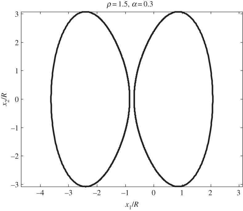
The shapes of the two holes by setting ρ=1.5 and α=0.3 in equation (5.32).

Figure 5.

The shapes of the two holes by setting ρ=1.5 and α=0.63i in equation (5.32).

Figure 6.

The variations of |ω^′(e^iθ)|/|R| (solid line) and its Fourier series expansion (circles) with ρ=1.5 and α=0.3 in equation (5.32).

6. Conclusion

In this paper, we have incorporated the effect of interface elasticity via the continuum-based Gurtin–Murdoch model into the interaction problem of a screw dislocation near an elastic inhomogeneity of arbitrary shape. The complexities of the discussed boundary value problem lie in the following aspects: (i) the elastic inhomogeneity is of arbitrary shape; (ii) the interface/surface elasticity is taken into account; (iii) the loadings include a screw dislocation in the matrix, remote uniform stresses and uniform eigenstrains imposed on the inhomogeneity. Despite these complexities, an elegant analytical solution has been obtained by means of complex variable techniques and matrix algebra. The size dependency of the elastic fields and image force on the dislocation have been clearly demonstrated from the solutions obtained. We have also incorporated the Gurtin–Murdoch model into the interaction problem of a screw dislocation in the vicinity of two closely spaced holes of irregular shape. An elegant solution to this interaction problem has been derived. The induced stress field and image force rely on two size-dependent parameters γ₁ and γ₂.

Funding statement

This work is supported by the National Natural Science Foundation of China (grant no. 11272121) and through a Discovery Grant from the Natural Sciences and Engineering Research Council of Canada.

References

- 1.Dundurs J. 1969. Elastic interaction of dislocations with inhomogeneities. In Mathematical theory of dislocations, (ed. Mura T.), pp. 70–115 New York, NY: ASME [Google Scholar]
- 2.Luo J, Xiao ZM. 2009. Analysis of a screw dislocation interacting with an elliptical nano inhomogeneity. Int. J. Eng. Sci. 47, 883–893 (doi:10.1016/j.ijengsci.2009.05.007) [Google Scholar]
- 3.Ahmadzadeh-Bakhshayesh H, Gutkin MY, Shodja HM. 2012. Surface/interface effects on elastic behavior of a screw dislocation in an eccentric core–shell nanowire. Int. J. Solids Struct. 49, 1665–1675 (doi:10.1016/j.ijsolstr.2012.03.020) [Google Scholar]
- 4.Gurtin ME, Murdoch A. 1975. A continuum theory of elastic material surfaces. Arch. Ration. Mech. Anal. 57, 291–323 (doi:10.1007/BF00261375) [Google Scholar]
- 5.Gurtin ME, Weissmuller J, Larche F. 1998. A general theory of curved deformable interface in solids at equilibrium. Philos. Mag. A 78, 1093–1109 (doi:10.1080/01418619808239977) [Google Scholar]
- 6.Ru CQ. 2010. Simple geometrical explanation of Gurtin–Murdoch model of surface elasticity with clarification of its related versions. Sci. China 53, 536–544 [Google Scholar]
- 7.Sharma P, Ganti S. 2004. Size-dependent Eshelby's tensor for embedded nano-inclusions incorporating surface/interface energies. ASME J. Appl. Mech. 71, 663–671 (doi:10.1115/1.1781177) [Google Scholar]
- 8.Sharma P, Ganti S, Bhate N. 2003. Effect of surfaces on the size-dependent elastic state of nano-inhomogeneities. Appl. Phys. Lett. 82, 535–537 (doi:10.1063/1.1539929) [Google Scholar]
- 9.Chen T, Dvorak GJ, Yu CC. 2007. Size-dependent elastic properties of unidirectional nano-composites with interface stresses. Acta Mech. 188, 39–54 (doi:10.1007/s00707-006-0371-2) [Google Scholar]
- 10.Tian L, Rajapakse RKND. 2007. Analytical solution for size-dependent elastic field of a nanoscale circular inhomogeneity. ASME J. Appl. Mech. 74, 568–574 (doi:10.1115/1.2424242) [Google Scholar]
- 11.Tian L, Rajapakse RKND. 2007. Elastic field of an isotropic matrix with a nanoscale elliptical inhomogeneity. Int. J. Solids Struct. 44, 7988–8005 (doi:10.1016/j.ijsolstr.2007.05.019) [Google Scholar]
- 12.Kim CI, Schiavone P, Ru C-Q. 2010. The effects of surface elasticity on an elastic solid with mode-III crack: complete solution. ASME J. Appl. Mech. 77, 021011 (doi:10.1115/1.3177000) [Google Scholar]
- 13.Kim CI, Schiavone P, Ru C-Q. 2011. The effects of surface elasticity on mode-III interface crack. Arch. Mech. 63, 267–286 [Google Scholar]
- 14.Kim CI, Schiavone P, Ru C-Q. 2011. Effect of surface elasticity on an interface crack in plane deformations. Proc. R. Soc. A 467, 3530–3549 (doi:10.1098/rspa.2011.0311) [Google Scholar]
- 15.Wang GF, Wang TJ, Feng XQ. 2006. Surface effects on the diffraction of plane compressional waves by a nanosized circular hole. Appl. Phys. Lett. 89, 231923 (doi:10.1063/1.2403899) [Google Scholar]
- 16.Wang GF, Wang TJ. 2006. Deformation around a nanosized elliptical hole with surface effect. Appl. Phys. Lett. 89, 161901 (doi:10.1063/1.2362988) [Google Scholar]
- 17.Wang X, Schiavone P. 2013. Surface effects in the deformation of an anisotropic elastic material with nano-sized elliptical hole. Mech. Res. Commun. 52, 57–61 (doi:10.1016/j.mechrescom.2013.06.007) [Google Scholar]
- 18.Ting TCT. 1996. Anisotropic elasticity-theory and applications Oxford, UK: Oxford University Press [Google Scholar]
- 19.Gao CF, Noda N. 2004. Faber series method for two-dimensional problems of arbitrarily shaped inclusion in piezoelectric materials. Acta Mech. 171, 1–13 (doi:10.1007/s00707-004-0131-0) [Google Scholar]
- 20.Wang X, Sudak LJ. 2006. Interaction of a screw dislocation with an arbitrary shaped elastic inhomogeneity. ASME J. Appl. Mech. 73, 206–211 (doi:10.1115/1.2073307) [Google Scholar]
- 21.Shen H, Schiavone P, Ru CQ, Mioduchowski A. 2000. An elliptic inclusion with imperfect interface in anti-plane shear. Int. J. Solids Struct. 37, 4557–4575 (doi:10.1016/S0020-7683(99)00174-2) [Google Scholar]