DOSE-FINDING WITH DRUG COMBINATIONS IN CANCER PHASE I CLINICAL TRIALS USING CONDITIONAL ESCALATION WITH OVERDOSE CONTROL (EWOC)

Abstract

We present a Bayesian adaptive design for dose finding of a combination of two drugs in cancer phase I clinical trials. The goal is to estimate the maximum tolerated dose (MTD) as a curve in the two-dimensional Cartesian plane. We use a logistic model to describe the relationship between the doses of the two agents and the probability of dose limiting toxicity. The model is re-parameterized in terms of parameters clinicians can easily interpret. Trial design proceeds using univariate escalation with overdose control, where at each stage of the trial, we seek a dose of one agent using the current posterior distribution of the MTD of this agent given the current dose of the other agent. At the end of the trial, an estimate of the MTD curve is proposed as a function of Bayes estimates of the model parameters. We evaluate design operating characteristics in terms of safety of the trial design and percent of dose recommendation at dose combination neighborhoods around the true MTD curve. We also examine the performance of the approach under model misspecifications for the true dose-toxicity relationship.

1. INTRODUCTION

Cancer phase I clinical trials are preliminary studies of cytotoxic and biologic agents administered to patients with advanced form of cancer who have exhausted all standard and conventional therapy [1]. Due to safety concerns and ethical considerations, these trials enroll patients sequentially and dose allocation to subsequent patients depends on the doses given to previously treated patients and their observed dose limiting toxicity (DLT) outcome by the end of the first cycle of therapy. Typically, the length of a cycle of therapy varies between 3 and 6 weeks, and may be longer for concurrent treatments with radiation therapy. Since treatment efficacy is assessed after several cycles of therapy, the primary objective of a phase I oncology trial is to estimate a maximum tolerable dose (MTD) of a new drug or combination of drugs for future efficacy evaluation in phase II/III trials. For the case of a single agent trial, the MTD, γ, is the dose that will produce DLT in a prespecified proportion θ of patients [2],

$$\mathrm{Prob}(\mathrm{DLT}|\mathrm{Dose}=\gamma )=\theta .$$ (1.1)

The definition of DLT depends on the type of cancer and drug under study but it is typically defined as a grade 3 or 4 non-hematologic and grade 4 hematologic toxicity, see the National Cancer Institute (NCI) common toxicity criteria [3] for the definition of the different grades of toxicity. The target probability of DLT θ depends on the nature and severity of treatment-attributable toxicity with common values selected in the interval [0.2, 0.4]. Single agent dose finding designs for cancer phase I clinical trials that are based on statistical models have been studied extensively in the last two decades, see for example [4] and [5] for a review.

The importance of drug combination therapy to treat malignant tumors has been known in the 1960s. For instance, James Holland, Emil Freireich, and Emil Frei hypothesized in 1965 that cancer chemotherapy should follow the strategy of antibiotic therapy for tuberculosis with combinations of drugs [6]. Combining several drugs can help reduce tumor resistance to chemotherapy by targeting different signaling pathways simultaneously and improve tumor response when using additive or synergistic drugs. Although the majority of phase I trials use drug combinations of several cytotoxic/biologic agents, most of them are designed to estimate the MTD of a single agent for fixed dose levels of the other agents. This approach may provide a single safe dose for the combination but it may be suboptimal in terms of therapeutic effects. A challenging problem in early phase dose finding trials is to identify a subset of dose combinations among a larger set of permissible dose combinations that will produce the same DLT rate. The general problem can be stated as follows. Let A_i, i = 1,…,k be k drugs and S_i Ϲ R⁺ be the set of all possible doses of drug A_i. Denote by x = (x₁,…, x_k) a dose combination of the k drugs and S = S₁×…× S_k. Consider a dose-toxicity model

$$\mathrm{Prob}\left(\mathrm{DLT}|\mathrm{dose}=\mathit{x}\right)=F(\mathit{x},\mathit{\xi }),$$ (1.2)

where F is a link function and ξ ε R^d is an unknown parameter. The MTD is defined as the set C of dose combinations x such that the probability of DLT for a patient given dose combination x equals to a target probability of DLT θ:

$$C=\left\{\mathit{x}\in S:F(\mathit{x},\mathit{\xi })=\theta \right\}.$$ (1.3)

A cancer phase I trial design is an algorithm of dose combination assignment to successive cohorts of patients in order to estimate the set C while minimizing the number of patients experiencing severe dose related side effects. Strategies for estimating C or subsets of C have been studied and used in real clinical trials by [7-10]. Design operating characteristics of these methods were not studied and their performance may be limited. For instance, in [7], the toxicity profile of each drug when used as a single agent is required and in [10], a single MTD is determined at the end of the trial. Parametric model based designs which explicitly describe the dose combination-toxicity relationship have been studied extensively in the last decade. Thall et al. [11] propose a six parameter model to represent the dose-toxicity relationship and a two-stage procedure was devised to allocate dose combinations of two agents. In the first stage, dose escalation proceeds along a diagonal using a pre-specified discrete set of dose combinations and in the second stage, toxicity contours are estimated and updated as DLT responses are accumulated. Wang and Ivanova [12] used a three-parameter regression model and estimate the MTD of one agent for each dose of the second agent. Yin and Yuan [13, 14] used copula-type models to describe the dose combination-toxicity relationship. At each stage of the trial, the dose combination to be allocated to the next patient is selected from a pre-specified neighborhood structure of dose combinations of the current dose according to the distance between the estimated probability of DLT of each neighboring dose combination and the target probability of DLT. Braun and Wang [15] use a Bayesian hierarchical structure to model the probability of DLT of all possible dose combinations and dose assignments proceeds using similar ideas described above, i.e., compare the estimated probabilities of DLT at neighboring dose combinations to the target probability of DLT. Wages et al. [16, 17] apply the idea of the continual reassessment method (CRM) [18] to the partial ordering of dose combinations of two agents. The idea is to pre-specify a set of possible orderings of the dose combinations, model the dose-toxicity relationship for each ordering, and assign prior probabilities for each of these models and each model parameter. At each stage of the trial, CRM is then applied to the model with the highest posterior probability. Sweeting and Mander [19] use the models proposed in [11] and [13] and investigate several dose allocation strategies during the trial and argued for the inclusion of moves that escalate both agents simultaneously. Shi and Yin [20] used univariate escalation with overdose control to allocate dose combinations to the next cohort of patients. In the presence of a large number of possible dose combinations, they used a sample size of n = 150 to derive design operating characteristics, which is impractical in cancer phase I clinical trials. By design, all of the methods mentioned above do not apply to the case of continuous dose levels of the two agents. Although the method of [11] can be used for continuous agents in the second stage of the trial, the first stage of the design does require a discretization of the dose combinations along a diagonal. Moreover, it is not clear how these methods will perform in the presence of a large number of dose combinations in relation to the sample size in the trial, especially if dose escalation by more than one level in either direction is not allowed.

In this article, we propose a Bayesian adaptive dose finding design in order to estimate the MTD curve of two agents with continuous dose levels. We use a logistic model to describe the dose-toxicity relationship and we reparameterize the model in terms of parameters clinicians can easily interpret. Trial design proceeds using univariate escalation with overdose control (EWOC), where at each stage of the trial, we seek a dose of one agent using the current posterior distribution of the MTD of this agent given the current dose of the other agent. Statistical properties and extensions of single agent EWOC are well understood, and have been studied in [21], [22], [23], [24], [25], [26],[27], and [28]. The defining property of EWOC is that at each stage of the trial, we seek a dose for which the posterior probability of exceeding the MTD is bounded by some feasibility bound α. At the end of the trial, an estimate of the MTD curve is proposed as a function of Bayes estimates of the model parameters.

The manuscript is organized as follows. In section 2, we give a detailed description of the Bayesian model and describe the adaptive trial design. In section 3, we study the performance of the proposed methodology in terms of safety of the trial and efficiency of the estimate of the MTD under a large number of scenarios and model misspecification. Section 4 contains some final remarks and discussion of practical implementations.

2. METHOD

2.1. DOSE-TOXICITY MODEL

Consider the problem of identifying a tolerable dose(s) of the combination of two cytotoxic agents A and B. Suppose that the doses of agents A and B are continuous and standardized to be in the interval [0, 1]. We consider the dose-toxicity model of the form

$$\mathrm{Prob}(Z=1|x,y)=F(\mu +\beta x+\gamma y+\eta xy),$$ (2.1)

where Z is the indicator of DLT, Z = 1 if a patient given the dose combination (x,y) exhibits DLT within one cycle of therapy, and Z = 0 otherwise, x is the dose level of agent A, y is the dose level of agent B, and F is a known cumulative distribution function.

We will assume that that the probability of DLT increases with the dose of any one of the agents when the other one is held constant. A sufficient condition for this property to hold is to assume β > 0 and γ > 0 and the interaction term η is nonnegative. The MTD is defined as any dose combination (x*, y*) such that

$$\mathrm{Prob}(Z=1|x^{\ast },y^{\ast })=\theta .$$ (2.2)

The value of the target probability θ is pre-specified by the clinicians and depends on the nature and clinical manageability of the DLT; it is set relatively high when the DLT is a transient, reversible or non-fatal condition, and low when it is life threatening. It follows from (2.1) and (2.2) that the MTD is the set of dose combinations

$$C=\left\{(x^{\ast },y^{\ast }):0\le x^{\ast },y^{\ast }\le 1,y^{\ast }=\frac{F^{-1}(\theta )-\mu -\beta x^{\ast }}{\gamma +\eta x^{\ast }}\right\}.$$ (2.3)

The MTD is a hyperbola in the Cartesian plane or a decreasing line in the absence of interaction between the two drugs.

We reparameterize model (2.1) in terms of Γ_A∣0, the MTD of drug A when the level of drug B is at its lowest available dose, Γ_B∣0, the MTD of drug B when the level of drug A is at its lowest available dose, ρ₀₀, the probability of DLT at the minimum available doses of agents A and B corresponding to x = y = 0, and the interaction parameter η. This reparameterization is convenient to clinicians since prior information on ρ₀₀, Γ_A∣0, and Γ_B∣0 may be available from other trials. In particular, under the Bayesian paradigm, if MTD estimates of single agent trials using A and B are available, then these estimates can be used to approximate the prior mean and variances of the parameters Γ_A∣0, and Γ_B∣0. In this manuscript, we will assume that 0 ≤ Γ_A∣0, Γ_B∣0 ≤ 1, i.e., the MTD of each agent when the other one is held at its minimum available dose in the trial is within the range of available doses in the trial. It can be shown that

$$\{\begin{array}{l}\mu =F^{-1}({\rho }_{00})\\ \beta =(F^{-1}(\theta )-F^{-1}({\rho }_{00}))/{\Gamma }_{A\mid 0}.\\ \gamma =(F^{-1}(\theta )-F^{-1}({\rho }_{00}))/{\Gamma }_{B\mid 0}\end{array}$$ (2.4)

The MTD in (2.3) becomes

$$C=\left\{(x^{\ast },y^{\ast }):0\le x^{\ast },y^{\ast }\le 1,y^{\ast }=\frac{\left(F^{-1}(\theta )-F^{-1}({\rho }_{00})\right)\left(1-x^{\ast }/{\Gamma }_{A\mid 0}\right)}{\left(\left(F^{-1}(\theta )-F^{-1}({\rho }_{00})\right)/{\Gamma }_{B\mid 0}\right)+\eta x^{\ast }}\right\}.$$ (2.5)

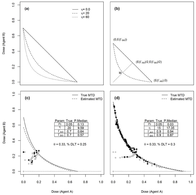
Figure 1(a) shows some MTD curves when ρ₀₀ = 0.05, Γ_A∣0 = 0.7, Γ_B∣0 = 0.7, and three values for the interaction coefficient η = 0, 20, 60 assuming that the target probability of DLT is θ = 0.33 and the link function is the logistic F(u) = (1 + e^−u)⁻¹.

Figure 1.

Let D_n = {(x_i,y_i,z_i), i = 1, …, n} be the data after enrolling n patients in the trial. The likelihood function for the model parameters is

$$\begin{array}{ll}L({\rho }_{00},{\Gamma }_{A\mid 0},{\Gamma }_{B\mid 0},\eta |D_n)=& {\prod _{i=1}^n\left(F({\rho }_{00},{\Gamma }_{A\mid 0},{\Gamma }_{B\mid 0},\eta ;x_i,y_i)\right)}^{z_i}\\ & \times {\left(1-F({\rho }_{00},{\Gamma }_{A\mid 0},{\Gamma }_{B\mid 0},\eta ;x_i,y_i)\right)}^{1-z_i},\end{array}$$ (2.6)

where

$$\begin{array}{l}F({\rho }_{00},{\Gamma }_{A\mid 0},{\Gamma }_{B\mid 0},\eta ;x_i,y_i)\\ =F\left(F^{-1}({\rho }_{00})+\frac{F^{-1}(\theta )-F^{-1}({\rho }_{00})}{{\Gamma }_{A\mid 0}}{x}_i+\frac{F^{-1}(\theta )-F^{-1}({\rho }_{00})}{{\Gamma }_{B\mid 0}}{y}_i+\eta x_i{y}_i\right).\end{array}$$ (2.7)

2.2. PRIOR AND POSTERIOR DISTRIBUTIONS

Equation (2.4) implies that 0 < ρ₀₀ < θ since β > 0. We assume that ρ₀₀, Γ_A∣0, Γ_B∣0, and η are independent a priori with ρ₀/θ ~ beta(a₁, b₁), Γ_A∣0 ~ beta(a₂, b₂), Γ_B∣0 ~ beta(a₃, b₃), and η ~ gamma(a, b) with mean E(η) = a / b and variance Var(η) = a / b². Under lack of prior information about the probability of DLT at the minimum dose combination (0, 0) and the MTDs of agents A and B when used as single agents, we take a_j = b_j = 1, j = 1, 2, 3 which corresponds to a uniform prior for ρ₀₀ in [0, θ] and uniform priors for the parameters Γ_A∣0, Γ_B∣0 in [0, 1].

We propose the following ad hoc procedure to specify the hyperparameters of the gamma prior distribution for the interaction coefficient η. In order to select the prior mean for η, substitute the prior mean values of ρ₀₀, Γ_A∣0, Γ_B∣0 in place of these parameters in (2.5) and consider the MTD curve passing through the three points with coordinates (0, E(Γ_B∣0)), (E(Γ_A∣0), 0), (E(Γ_A∣0)/4, E(Γ_B∣0)/4). The prior mean of η is solution to the equation

$$E({\Gamma }_{B\mid 0})/4=\frac{\left(F^{-1}(\theta )-F^{-1}(E({\rho }_{00}))\right)\left(1-\left(E({\Gamma }_{A\mid 0})/4\right)/E({\Gamma }_{A\mid 0})\right)}{\left(\left(F^{-1}(\theta )-F^{-1}({\rho }_{00})\right)/E({\Gamma }_{B\mid 0})\right)+E(\eta )E({\Gamma }_{A\mid 0})/4}.$$ (2.8)

It follows that

$$E(\eta )=\frac{8\left(F^{-1}(\theta )-F^{-1}(E({\rho }_{00}))\right)}{E({\Gamma }_{A\mid 0})E({\Gamma }_{B\mid 0})}.$$ (2.9)

The idea here is to draw the MTD curve passing through the point of average MTDs (E(Γ_A∣0), 0) and (0, E(Γ_B∣0)) when the interaction coefficient is 0, see the solid line in Figure 1(b). Then, draw the dotted line passing through (0, 0) and the midpoint of the solid line. MTD curves passing through the points of average MTDs (E(Γ_A∣0), 0) and (0, E(Γ_B∣0)) will cross the dotted line as η increases. Among these curves, we select the one passing through the midpoint M of the dotted line with coordinates (E(Γ_A∣0)/4, E(Γ_B∣0)/4). This curve is shown by a dashed line in Figure 1(b). The value of η corresponding to this MTD curve is found by solving equation (2.8), and the solution is selected as the prior expected value for η, and is given by (2.9). A large variance is selected for this prior.

Using Bayes rule, the posterior distribution of the model parameters is proportional to the product of the likelihood and prior distribution

$$\begin{array}{ll}\pi ({\rho }_{00},{\Gamma }_{A\mid 0},{\Gamma }_{B\mid 0},\eta & \mid D_n)\propto \prod _{i=1}^n{\left(F({\rho }_{00},{\Gamma }_{A\mid 0},{\Gamma }_{B\mid 0},\eta ;x_i,y_i)\right)}^{z_i}\\ & \times {\left(1-F({\rho }_{00},{\Gamma }_{A\mid 0},{\Gamma }_{B\mid 0},\eta ;x_i,y_i)\right)}^{1-z_i}{\rho }_{00}^{a_1-1}{\left(1-{\rho }_{00}\right)}^{b_1-1}\\ & \times {\left({\Gamma }_{A\mid 0}\right)}^{a_2-1}{\left(1-{\Gamma }_{A\mid 0}\right)}^{b_2-1}{\left({\Gamma }_{B\mid 0}\right)}^{a_3-1}{\left(1-{\Gamma }_{B\mid 0}\right)}^{a_3-1}{\eta }^{a-1}{e}^{-\mathit{b\eta }}.\end{array}$$ (2.10)

We used WinBUGS [29] and JAGS to estimate features of the posterior distribution of these parameters and estimate design operating characteristics of cancer phase I trials described below.

2.3. TRIAL DESIGN

Dose escalation/de-escalation is designed so that at each stage of the trial, one of the agents is held constant while seeking a dose for the other agent using EWOC. For example, if agent A is held constant at level x, the dose of agent B is y such that the posterior probability that y exceeds the MTD of agent B given that the dose of agent A is x equals to a feasibility bound α. Specifically, the design proceeds as follows:

1. The first patient receives dose (x₁, y₁) = (0, 0) and suppose the patient has no DLT, z₁ = 0.

2. Fix x₁ = 0, and calculate the posterior distribution of the MTD of agent B, given that the level of agent A is x₁ = 0, π(Γ_B∣A=0 ∣ D₁). The dose for patient 2 is (x₂, y₂) where x₂ = x₁ and y₂ is the α-th percentile of this posterior distribution.

3. Fix y₂, and calculate the posterior distribution of the MTD of agent A, given that the level of agent B is y₂, π(Γ_A∣B=y2 ∣ D₂). The dose for patient 3 is (x₃, y₃) where x₃ is the α-th percentile of this posterior distribution and y₃ = y₂.

In general, when we move from dose (x_i, y_i) to (x_i+1, y_i+1), either x_i = x_i+1 or y_i = y_i+1. Specifically, if i is even, then $x_{i+1}={\Pi }_{{\Gamma }_{A\mid B=y_i}}^{-1}(\alpha \mid D_i)$ and y_i+1 = y_i. If i is odd, then x_i+1 = x_i and $y_{i+1}={\Pi }_{{\Gamma }_{B\mid A=x_i}}^{-1}(\alpha \mid D_i)$. Here, ${\Pi }_{{\Gamma }_{A\mid B=y_i}}^{-1}(\alpha \mid D_i)$ is the inverse cdf of the posterior distribution π(Γ_A∣B=yi ∣ D_i). Details for estimating features of this posterior distribution are included in the appendix.

• 4Repeat step 3 by fixing either dose x_i or y_i, depending on whether i is even or odd, until n patients are enrolled to the trial.

In step 2, one can fix y₁ instead of x₁ and proceed in a similar manner. At the end of the trial, we estimate the MTD using (2.5) as

$$\widehat{C}=\left\{(x^{\ast },y^{\ast }):0\le x^{\ast },y^{\ast }\le 1,y^{\ast }=\frac{\left(F^{-1}(\theta )-F^{-1}({\widehat{\rho }}_{00})\right)\left(1-x^{\ast }/{\widehat{\Gamma }}_{A\mid 0}\right)}{\left(\left(F^{-1}(\theta )-F^{-1}({\widehat{\rho }}_{00})\right)/{\widehat{\Gamma }}_{B\mid 0}\right)+\widehat{\eta }{x}^{\ast }}\right\},$$ (2.11)

where ρ̂₀, Γ̂_A∣0, Γ̂_B∣0, η̂ are the posterior medians given the data D_n.

Figure 1(c) shows an example of a simulated trial enrolling n = 40 patients using a logistic link function F(u) = (1 + e^−u)⁻¹ and target probability of DLT θ = 0.33. Uniform priors for ρ₀₀, Γ_A∣0, Γ_B∣0 were used and using (2.9), the prior mean for η is E(η) = 30. We took Var(η) = 900. We used a variable feasibility bound α, starting with α = 0.25 and increase this value in increments of 0.05 each time we compute the dose for the next patient until α = 0.5, see [30, 31] for the rationale for selecting a variable feasibility bound. Starting with the dose combination (0, 0), this figure shows how the sequence of doses moves along a vertical-horizontal path as it tends to get closer to the true MTD curve shown by a solid line. The estimated MTD curve shown by a dashed line is found using (2.11). At the conclusion of the trial, 25% of the patients exhibited DLT. Figure 1(d) shows another example of a hypothetical simulated trial enrolling n = 300 patients using the same link function and prior distributions except that Var(η) = 225. This example shows that eventually, patients will be assigned dose combinations very close to the true MTD curve. In both cases, DLT responses were generated from the logistic dose-toxicity model.

3. SIMULATION STUDIES

3.1 SIMULATION SET UP AND SCENARIOS

We evaluate design operating characteristics by assuming a logistic link function F(u) = (1 + e^−u)⁻¹ to model the dose-toxicity relationship. DLT responses are generated assuming both a logistic link function and three other link functions to assess the performance of the method under model misspecification. These are (1) the probit link F(u) = Φ(u), where Φ(·) is the cdf of the standard normal distribution, (2) the normal link F(u) = Φ(u/σ), and (3) the complementary log-log link F(x) =1−e^−ex. Model misspecification under a family of models which does not belong to (2.1) is included in the supplement. In all simulations, the target probability of DLT is fixed at θ = 0.33 and the trial sample size is n = 40 patients. We considered 10 scenarios corresponding to a fixed true value for ρ₀₀ = 0.05, two values for the interaction coefficient η = 5, 20, and five combinations of (Γ_A∣0, Γ_B∣0), {(0.2, 0.2), (0.4, 0.4), (0.6, 0.6), (0.8, 0.8), (0.8, 0.5)}. These scenarios reflect different locations for the true MTD curve in the Cartesian plane with varying distances from the initial dose.

We used uniform priors for ρ₀₀, Γ_A∣0, Γ_B∣0 to reflect a lack of prior knowledge about the toxicity profiles of the two agents and using (2.9), the prior mean for η is E(η) = 30. We took a large prior variance for η, Var(η) = 900. For each scenario, we simulated m = 1000 trials by generating the DLT responses from each of the four models logistic, probit, normal with σ = 2, and complementary log-log. The parameter values μ, β, γ, η of these models were selected in such a way that they all have the same true MTD curve. Figure 2 illustrates the extent of departures of these models from the logistic dose-toxicity model under the scenario ρ₀₀ = 0.05, Γ_A∣0 = Γ_B∣0 = 0.8, and η = 5. In each panel, the solid curve represents the true MTD common to all models and each figure includes contour plots corresponding to different probabilities of DLT. The probabilities of DLT of the toxicity profiles of the logistic model are shown in bold italic below the diagonal and the corresponding probabilities for the other models are included above the diagonal. The top-left panel of Figure 2 shows a case where the DLT responses are generated from a model with tighter toxicity profiles relative to the assumed logistic model. The top-right panel is a situation where the logistic dose-toxicity model is tighter relative to the normal model and the bottom-left panel of Figure 2 is a case where the logistic model is wider relative to the complementary log-log model above the MTD curve but is tighter compared to this model below the MTD curve. We feel that these scenarios and model misspecifications cover a wide range of practical situations and are reasonable to evaluate the performance and robustness of the methodology.

Figure 2.

3.2. DESIGN OPERATING CHARACTERISTICS

For each scenario, we present an estimate of the MTD curve

$$\overline{C}=\left\{(x^{\ast },y^{\ast }):0\le x^{\ast },y^{\ast }\le 1,y^{\ast }=\frac{\left(F^{-1}(\theta )-F^{-1}({\overline{\rho }}_{00})\right)\left(1-x^{\ast }/{\overline{\Gamma }}_{A\mid 0}\right)}{\left(\left(F^{-1}(\theta )-F^{-1}({\overline{\rho }}_{00})\right)/{\overline{\Gamma }}_{B\mid 0}\right)+\overline{\eta }{x}^{\ast }}\right\},$$ (3.1)

where F(·) is the logistic function and ρ̄₀₀, Γ̄_A∣0, Γ̄_B∣0, η̄ are the average posterior medians of the parameters ρ₀₀, Γ_A∣0, Γ_B∣0, η from all m = 1000 trials. For trial safety, we present the percent of DLTs across all patients and all trials, the percent of trials with DLT rate greater than θ + 0.1. For trial efficiency, we first select six points corresponding to six dose combinations equally spaced on the true MTD curve. For each point (x,y), find the Euclidian distance Δ(x,y) between the origin (minimum doses of the two agents) and this point. Draw a circle with radius pΔ(x,y) and center (x,y), 0 < p < 1. For each circle, we calculate the percent of trials with MTD curve estimate falling inside the circle. This will give us the percent of trials with MTD recommendation within (100×p)% of the true MTD. We will select p = 0.1, 0.2. Such measure of efficiency has been used for single agent phase I trial designs with a continuous dose by [32]. The bottom-right panel of Figure 2 illustrates the variability of the radius of the tolerance circles for various locations of dose combinations on the true MTD curve under two different scenarios ρ₀₀ = 0.05, η = 5, Γ_A∣0 = Γ_B∣0 = 0.2, and Γ_A∣0 = Γ_B∣0 = 0.8. Here, p = 0.1. We can see that the farther the true MTD is from the minimum dose combination, the larger is the tolerance for estimating the percent of MTD recommendation. Another measure of efficiency we consider is the pointwise average relative minimum distance from the true MTD curve to the estimated MTD curve. This is defines as follows: For i = 1,…,m, let C_i be the estimated MTD curve and let C_true be the true MTD curve. For every point (x,y) ε C_true, let

$$d_{(x,y)}^{(i)}=\mathit{sign}(y^{\prime }-y)\times \underset{\left\{(x^{\ast },y^{\ast }):(x^{\ast },y^{\ast })\in C_i\right\}}{\min }{\left({(x-x^{\ast })}^2+{(y-y^{\ast })}^2\right)}^{1/2}$$ (3.2)

where y′ is such that (x, y′) ε C_i. This represents the minimum relative distance of the point (x,y) on the true MTD curve to the estimated MTD curve C_i. If the point (x,y) is below C_i, then $d_{(x,y)}^{(i)}$ is positive. Otherwise, it is negative. Let

$$d_{(x,y)}=m^{-1}\sum _{i=1}^m{d}_{(x,y)}^{(i)}.$$ (3.3)

This is the pointwise average relative minimum distance from the true MTD curve to the estimated MTD curve which can be interpreted as the pointwise average bias in estimating the MTD. The last measure of efficiency we consider is

$$m^{-1}\sum _{i=1}^{m}I\left(|d_{(x,y)}^{(i)}|\le p\mathrm{\Delta }(x,y)\right).$$ (3.4)

This is the pointwise percent of trials for which the minimum distance of the point (x,y) on the true MTD curve to the estimated MTD curve C_i is no more than (100×p)% of the true MTD. This is equivalent to the statistic summarizing the percent of trials falling inside a given circle described above and can be interpreted as the pointwise percent of MTD recommendation for a given tolerance p.

3.3. RESULTS

3.3.1 Trial Safety

Table 1 shows that the average percent of DLTs varies between 19% and 34% across all scenarios. This average DLT rate tends to be lower when the true MTD curve is farther away from the minimum dose combination, consistent with the results of single agent trials using EWOC, see [23] and [28]. Table 1 also shows that the percent of trials with an excessive number of DLTs as defined by a DLT rate exceeding θ + 0.1 is very small with the highest value of 3.2% achieved when the true MTD curve is very close to the minimum dose combination available in the trial, Γ_A∣0 = Γ_B∣0 = 0.2. Based on these findings, we conclude that the methodology is safe in general.

Table 1.

Design operating characteristics under 10 scenarios. A neighborhood of a point (x, y) is defined as an open circle with center (x,y) and radius p×Δ(x,y) where Δ(x,y) is the Euclidian distance between the origin and (x, y) and p = 0.2.

Scenario # (ΓA∣0, ΓB∣0, η)	Model	% trials with MTD recommendation in a neighborhood of each of the 6 points						Average %DLTs	% trials: DLT rate > θ+0.1
		1	2	3	4	5	6
1 (0.2, 0.2, 5)	Logistic	39.5	48.0	50.6	47.3	38.8	27.7	33	3.2
	Probit	42.3	49.9	48.1	40.7	27.8	16.5	33	0.1
	Normal	41.1	49.1	51.1	47.7	39.5	30.5	33	0.1
	LogLog	42.4	48.7	48.9	43.6	33.2	23.8	33	0.4
2 (0.4, 0.4, 5)	Logistic	80.1	79.5	77.0	78.3	79.8	79.2	26	0.0
	Probit	79.2	80.5	80.3	79.9	79.2	77.3	27	0.0
	Normal	78.2	76.5	72.0	73.6	76.8	76.1	26	0.0
	LogLog	78.8	79.6	78.2	78.4	78.7	77.9	26	0.0
3 (0.6, 0.6, 5)	Logistic	96.1	87.0	82.0	87.0	95.2	98.1	22	0.0
	Probit	97.6	93.1	90.8	92.9	96.2	99.3	23	0.0
	Normal	96.3	81.6	75.9	81.3	95.0	98.4	22	0.0
	LogLog	96.4	89.4	86.7	89.2	95.0	98.8	22	0.0
4 (0.8, 0.8, 5)	Logistic	99.7	89.1	85.6	92.6	99.9	100	19	0.0
	Probit	100	98.4	97.4	99.2	100	100	19	0.0
	Normal	99.5	81.7	77.5	87.0	99.6	100	20	0.0
	LogLog	99.9	92.8	90.5	95.3	100	100	19	0.0
5 (0.8, 0.5, 5)	Logistic	79.5	82.5	86.4	95.1	100	100	22	0.0
	Probit	72.0	86.4	97.2	99.8	100	100	22	0.0
	Normal	82.0	81.4	82.9	93.2	100	100	22	0.0
	LogLog	77.4	84.4	93.0	98.5	100	100	22	0.0
6 (0.2, 0.2, 20)	Logistic	43.1	46.9	45.3	41.2	34.5	26.9	34	0.7
	Probit	43.3	44.7	37.7	28.0	20.0	15.0	33	0.1
	Normal	42.3	47.0	46.4	43.7	37.1	28.5	34	1.2
	LogLog	46.3	47.7	43.3	36.6	28.8	21.8	33	0.5
7 (0.4, 0.4, 20)	Logistic	83.4	71.9	69.3	74.4	82.2	90.6	28	0.1
	Probit	87.5	76.7	73.8	78.3	86.2	93.8	28	0.0
	Normal	82.9	72.1	68.8	73.3	82.0	90.4	28	1.2
	LogLog	84.5	75.4	72.8	77.3	83.1	90.6	28	0.0
8 (0.6, 0.6, 20)	Logistic	95.1	78.6	82.5	93.8	99.2	99.8	25	0.0
	Probit	96.7	83.6	87.3	96.2	99.7	100	26	0.0
	Normal	93.8	76.4	79.8	93.5	98.8	100	26	0.0
	LogLog	95.9	79.0	83.2	94.7	99.4	100	26	0.0
9 (0.8, 0.8, 20)	Logistic	96.6	81.8	93.6	99.7	100	100	24	0.0
	Probit	99.5	88.0	97.4	100	100	100	24	0.0
	Normal	96.4	79.5	91.6	99.6	100	100	24	0.0
	LogLog	98.3	86.9	96.3	99.9	100	100	24	0.0
10 (0.8, 0.5, 20)	Logistic	77.4	79.5	97.4	100	100	100	25	0.0
	Probit	75.0	86.6	99.1	100	100	100	25	0.0
	Normal	78.3	80.4	95.6	99.6	99.6	99.8	25	0.0
	LogLog	73.4	82.2	98.0	100	100	100	25	0.0

3.3.2 Trial Efficiency

Table 1 gives the percent of trials with MTD recommendation within (100×p)% of the true MTD for selected points equally spaced on the true MTD curve with p = 0.2. In all cases, the next dose combination is calculated using the logistic link function and the DLT responses are generated from one of the four link functions logistic, probit, normal, and complementary log-log. The results for p = 0.1 are not included due to space limitation but equivalent measures for selected scenarios are included in Figure 5. The percent of MTD recommendation is very high in all scenarios except in the case where the true MTD curve is near the minimum dose combination. For instance, the percent recommendation in a neighborhood of the sixth dose combination is 27% when Γ_A∣0 = Γ_B∣0 = 0.2 and the DLT responses are generated from the true model with logistic link function. When the true MTD curve is farther away from the minimum dose combination, the estimated percent of trials with MTD recommendation within 20% of the true MTD is 80% or more, see scenarios 3, 4, 8, and 9. When the tolerance is reduced to p = 0.1, the percent of trials with MTD recommendation within 10% of the true MTD for these same scenarios varies between 45% and 100%.

Figure 5.

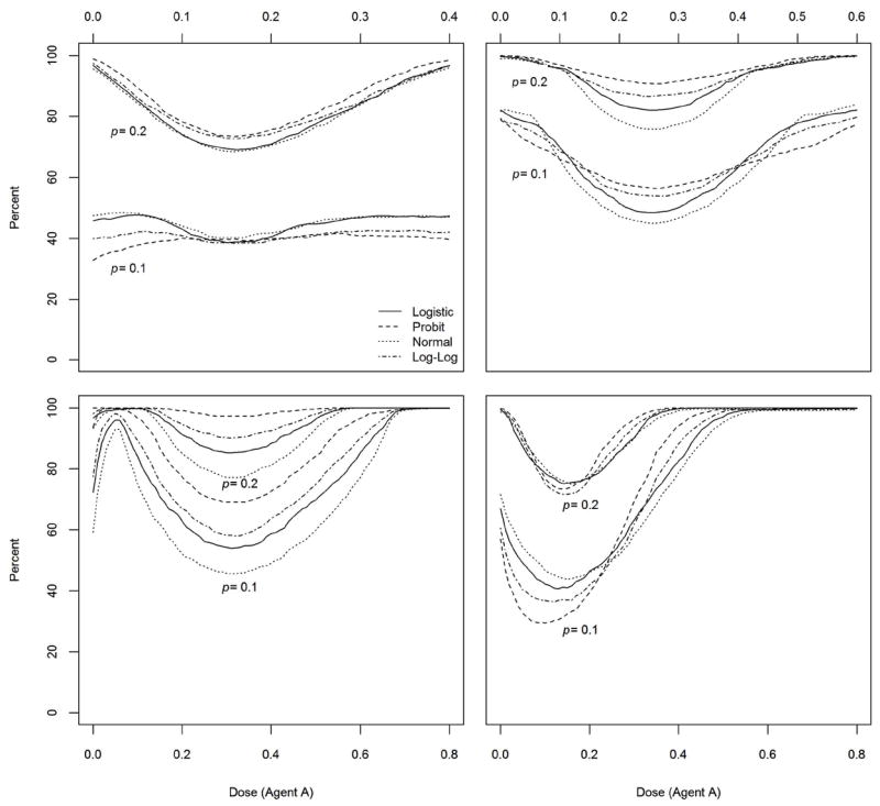
Figure 3 shows the plots of the true and estimated MTD curves under four selected scenarios as described by their true parameter values in each table within each panel of Figure 3. The second column of each table contains the true parameter values and the third column contains the average posterior medians of the parameters ρ₀₀, Γ_A∣0, Γ_B∣0, η from all m = 1000 trials. The estimated MTD curve shown by a dashed line was obtained using (3.1) and DLT responses were simulated using the true logistic model. We can see that the estimated MTD curve is close to the true MTD and the precision of the estimate is higher for high values of Γ_A∣0 and Γ_B∣0. When the true MTD curve is close to the minimum dose combination, for example when Γ_A∣0 = Γ_B∣0 = 0.2 (results not shown), the estimated MTD curve tends to be above the true MTD curve. This is probably due to the fact that we are using uniform priors for Γ_A∣0 and Γ_B∣0 with prior means equal to 0.5. In other words, no prior information about the agents when used as single drugs is being used except from the fact that we are assuming that the MTD of each agent when the level of the other agent is at its minimum value 0 is between 0 and 1. Each panel of Figure 3 also includes a scatter plot of the last dose combinations from each of the m = 1000 simulated trials along with 90% and 50% confidence regions. These statistics are useful for clinicians who plan to use the last dose combination in a phase I trial as the recommended phase II dose combinations as in [15].

Figure 3.

Figure 4 displays the pointwise average relative minimum distance from the true MTD curve to the estimated MTD curve as defined by (3.3) for selected scenarios. This is a measure of pointwise average bias of the estimate of the MTD. In the case Γ_A∣0 = Γ_B∣0 = 0.4 (top-left panel of Figure 4), the maximum average bias is about 0.042 when DLT responses are generated from the true logistic model. This corresponds to 10% of the distance from the minimum dose combination (0, 0) to the true MTD dose combination (0, 0.4). In the top right panel of Figure 4, the maximum average bias is about 6% of the distance from dose combination (0, 0) to the true MTD dose combination (0, 0.6). Similar measures of average bias are found in the bottom panels of Figure 4 with maximum values of 6.8% and 8.0% of the distance from (0, 0) to the true MTD dose combinations (0, 0.8) and (0, 0.5), respectively. In all cases, the average bias is smallest around the middle part of the true MTD curve. In fact, for sample size n = 40-60 patients, our experience with the simulation outputs of many other scenarios showed that for most trials, most patients in a trial will be assigned dose combinations scattered around the middle portion of the true MTD curve.

Figure 4.

Figure 5 shows the plots of the pointwise percent of trials for which the minimum distance from the true MTD curve to the estimated MTD curve is no more than (100×p)% of the true MTD for selected scenarios. In each panel, we present estimates based on the tolerances p = 0.1 and p = 0.2. The top left panel of Figure 5 shows that around 40% of the trials will recommend an MTD estimate that is within 10% of the true value of the MTD when the DLT responses are generated from the true logistic model. With a tolerance of p = 0.2, the percent of trials with correct MTD recommendation varies between 70% and 98%. Similar observations can be made in the case Γ_A∣0 = Γ_B∣0 = 0.6 (top-right panel) and Γ_A∣0 = Γ_B∣0 = 0.8 (bottom-left panel). The pointwise percent of MTD recommendation seems to increase as the true MTD curve drifts away from the minimum dose combination. In the last scenario Γ_A∣0 = 0.8 and Γ_B∣0 = 0.5, the percent of MTD recommendation is much higher for dose combinations for which the level of agent A is 0.4 or more. Based on these results and others from scenarios not shown here, we conclude that the design is practically efficient in general in recommending the MTD curve estimate.

3.3.3. Model Robustness

Table 1 shows that the average percent of DLTs across all trials are similar when the logistic model is misspecified. The largest difference in the percent of trials with DLT rates exceeding θ +0.1 between the logistic model and its three misspecifications equals to 3.1%. This occurs when the true MTD curve is close to the minimum dose combination with a relatively low synergy between the drugs (scenario 1) and the probit model is used to generate the DLT responses. In all other cases, these percentages are very close. We conclude that the method is fairly robust as far as trial safety is concerned.

In Figure 4, the largest absolute difference in the pointwise average bias is achieved when the DLT responses are generated from the probit model. The largest of these differences in achieved under scenario 3 corresponding to Γ_A∣0 = Γ_B∣0 = 0.6 and η = 5 at point x* with x-coordinate 0.25. This difference is just under 0.03, which is about 7% of the distance from the minimum dose combination to the point x* on the true MTD curve. Similar findings were seen in the remaining six scenarios not shown here. Figure 5 shows that the percent of MTD recommendations are fairly similar in most scenarios with the largest difference obtained when the DLT responses are generated from the probit model. The largest of these differences is around 13% and in achieved under scenario 4 corresponding to Γ_A∣0 = Γ_B∣0 = 0.8 and η = 5 when the level of drug A is about 0.35. We note that the probit model has toxicity contours that deviate the most from the logistic model as shown in Figure 2. We conclude that our method is fairly robust to model misspecifications under the dose-toxicity family of models of the form Prob(DLT ∣ x,y) = F(μ + β x + γ y + η x y) for some selected link functions F(·). Model misspecification under a six parameter model is included in the supplement. Finally, we computed the percent of trials for which the difference between consecutive dose escalations of either agent exceeds 0.1 (10% of the dose range of either agent) at least once after the second patient is enrolled to the trial. In all scenarios and under all model misspecifications, this percent was 0.00 indicating that the method prevents high jumps in dose assignments to future patients.

4. CONCLUSIONS

We proposed a Bayesian adaptive design for cancer phase I clinical trials using two drugs with continuous dose levels. The goal is to estimate the MTD curve in the two-dimensional Cartesian plane. To the best of our knowledge, this is the first method geared towards estimating the MTD curve based on continuous dose levels of the agents under consideration. The use of continuous dose levels is very common in clinical oncology research, especially when the agents are delivered as infusions intravenously. The previous methods which discretize the dose levels cannot be applied here since increasing the number of dose combinations of the agents will require large sample sizes, which is impractical in dose finding cancer trials. The method we presented is model based and the design alternates the use of single agent EWOC conditional on the dose level of the other agent. Prior information about the MTDs of each agent when used as single agents can be easily accounted for in the model but it is not required otherwise. Apart from the dose-toxicity model assumption we made, we only require that the MTDs Γ_A∣0 and Γ_B∣0 are within the range of doses available in the trial. We used vague priors for these parameters and proposed an ad hoc method to place a weakly informative prior distribution on the interaction term between the two drugs.

We studied design operating characteristics of the method under a large number of practical scenarios and under several model misspecifications. In all simulations, we used a sample size of n = 40 patients, close to the sample size of n = 35 used in [15]. Note that [11], [13, 14] all used n = 60. We found that in general, the methodology is safe in terms of the probability that a prospective trial will results in an excessively high number of DLTs. We used several measures to assess the efficiency of the estimate of the MTD and in the majority of scenarios, the percent of MTD recommendation is good and increases as the true MTD curve drifts away from the minimum dose combination. According to these results, the pointwise average bias is smallest around the middle of the MTD curve but the percent of MTD recommendation is higher at the extremes. This is probably due to the fact that the percent of MTD recommendation depends on the distance from the minimum dose combination to the MTD curve and this distance is highest at the extremes. We recommend that clinicians select dose combinations around the middle of the MTD curve for efficacy evaluation since the percent of recommendation is still high and dose combinations where the level of one of the agents is very low may not be of interest for efficacy studies. We also showed that the method is practically robust with respect to trial safety and efficiency under a reasonable class of model misspecification. We further emphasize here that unlike previously published methods, information of the toxicity profiles of agents A and B from single agent trials is not being used in the prior distributions of Γ_A∣0 and Γ_B∣0. If such information is available, then informative priors can be placed on Γ_A∣0 and Γ_B∣0 and we expect better model operating characteristics. Therefore, we conclude that this design has good operating characteristics for estimating the MTD curve of drug combinations of two agents with continuous dose level.

The assumption that the MTDs Γ_A∣0 and Γ_B∣0 are within the range of doses available in the trial may be restrictive, especially if agents A and B were never used as single agents in human phase I trials. We plan to relax this condition using alternative dose-toxicity models and model reparameterizations as in [23] in our future work. We also plan to study the performance of the proposed design under a class of models which allow synergistic and antagonistic relation between the drugs as described in [33]. Finally, we plan to assess the performance of the method when the doses of the two agents are discretized. We will use the same method discussed in [21] and [30] for dealing with a prespecified set of discrete dose level and we plan to compare the performance of the design with the methods described in [15, 16, 34, 35].

APPENDIX

Let Γ_A∣B=y be the MTD of agent A when the level of agent B is y and Γ_B∣A=x be the MTD of agent B when the level of agent A is x. Using (2.1) and (2.2), μ + βΓ_A∣B=y + γy + ηΓ_A∣B=y y = F⁻¹(θ). It follows that Γ_A∣B=y = (F⁻¹(θ) − μ − γy)/(β + ηy). Using the model reparameterization (2.4), we find

$${\Gamma }_{A\mid B=y}=\frac{\left(F^{-1}(\theta )-F^{-1}({\rho }_{00})\right)\left(1-y/{\Gamma }_{B\mid A=0}\right)}{\left(\left(F^{-1}(\theta )-F^{-1}({\rho }_{00})\right)/{\Gamma }_{A\mid B=0}\right)+\mathit{\eta y}}.$$

The parameter Γ_B∣A=x is found similarly. In order to calculate the next dose in steps 2 and 3 of the algorithm of the trial design, we truncate the posterior distributions of Γ_A∣B=y and Γ_B∣A=x to the intervals (0, Γ_A∣B=0) and (0, Γ_B∣A=0), respectively. Suppose that the dose combination given to the current patient is (x_i,y_i) and i is even. The dose for the next patient is (x_i+1,y_i+1) such that y_i+1 = y_i and P(Γ_A∣B=yi ≤ x_i+1 ∣ D_i) = α. The dose x_i+1 is the α-th percentile of the posterior distribution of Γ_A∣B=yi truncated to the interval (0, Γ_A∣B=0). Let ρ_00,l, Γ_A∣B=0,l, Γ_B∣A=0,l, η_l, l = 1, …, m be an MCMC sample from the posterior distribution in (2.10). Let S_m be the largest subset of {print], m} such that

$$\frac{\left(F^{-1}(\theta )-F^{-1}({\rho }_{00,j})\right)\left(1-y_i/{\Gamma }_{B\mid A=0,j}\right)}{\left(\left(F^{-1}(\theta )-F^{-1}({\rho }_{00,j})\right)/{\Gamma }_{A\mid B=0,j}\right)+{\eta }_j{y}_i}\in [0,{\Gamma }_{A\mid B=0,j}]$$

for all j in S_m. We estimate dose x_i+1 as the sample α-th percentile of the MCMC sample

$$\left\{{\widehat{\Gamma }}_{A\mid B=y_i}=\frac{\left(F^{-1}(\theta )-F^{-1}({\rho }_{00,j})\right)\left(1-y_i/{\Gamma }_{B\mid A=0,j}\right)}{\left(\left(F^{-1}(\theta )-F^{-1}({\rho }_{00,j})\right)/{\Gamma }_{A\mid B=0,j}\right)+{\eta }_j{y}_i},j\in S_m\right\}.$$

If i is odd, Γ̂_B∣A=xi, is computed similarly.

References

- 1.Roberts TG, Goulart BH, Squitieri L, Stallings SC, Halpern EF, Chabner BA, Gazelle GS, Finkelstein SN, Clark JW. Trends in the risks and benefits to patients with cancer participating in phase 1 clinical trials. Jama-Journal of the American Medical Association. 2004;292:2130–2140. doi: 10.1001/jama.292.17.2130. [DOI] [PubMed] [Google Scholar]
- 2.Gatsonis C, Greenhouse JB. Bayesian Methods for Phase-I Clinical-Trials. Statistics in Medicine. 1992;11:1377–1389. doi: 10.1002/sim.4780111011. [DOI] [PubMed] [Google Scholar]
- 3.National Cancer Institute. Common Toxicity Criteria for Adverse Events v3.0 (CTCAE) 2003 http://ctep.cancer.gov/reporting/ctc.html, City.
- 4.Ting N. Dose Finding in Drug Development. First edn. Springer; New York: 2006. [Google Scholar]
- 5.Chevret S. Statistical Methods for Dose-finding Experiments. Wiley; Chichester: 2006. [Google Scholar]
- 6.Frey E, III, Karon M, Levin RH, Freireich EJ, Taylor RJ, Hananian J, Selawry O, Holland JF, Hoogstraten B, Wolman IJ, Abir E, Sawitsky A, Lee S, Mills SD, Burgert EO, Spurr CL, Patterson RB, Ebaugh FG, James GWI, Moon JH. The Effectiveness of Combinations of Antileukemic Agents in Inducing and Maintaining Remission in Children with Acute Leukemia. Blood. 1965;26:642–656. [PubMed] [Google Scholar]
- 7.Korn EL, Simon R. Using the Tolerable-Dose Diagram in the Design of Phase-I Combination Chemotherapy Trials. Journal of Clinical Oncology. 1993;11:794–801. doi: 10.1200/JCO.1993.11.4.794. [DOI] [PubMed] [Google Scholar]
- 8.Lokich J. Phase I clinical trial of weekly combined topotecan and irinotecan. American Journal of Clinical Oncology-Cancer Clinical Trials. 2001;24:336–340. doi: 10.1097/00000421-200108000-00003. [DOI] [PubMed] [Google Scholar]
- 9.Kuzuya K, Ishikawa H, Nakanishi T, Kikkawa F, Nawa A, Fujimura H, Iwase A, Arii Y, Kawai M, Hattori S, Sakakibara K, Sasayama E, Furuhashi Y, Suzuki T, Mizutani S. Optimal doses of paclitaxel and carboplatin combination chemotherapy for ovarian cancer: a phase I modified continual reassessment method study. Int J Clin Oncol. 2001;6:271–278. doi: 10.1007/s10147-001-8027-7. [DOI] [PubMed] [Google Scholar]
- 10.Harvey RD, Owonikoko TK, Lewis CM, Akintayo A, Chen Z, Tighiouart M, Ramalingam SS, Fanucchi MP, Nadella P, Rogatko A, Shin DM, El-Rayes B, Khuri FR, Kauh JS. A phase 1 Bayesian dose selection study of bortezomib and sunitinib in patients with refractory solid tumor malignancies. British Journal of Cancer. 2013;108:762–765. doi: 10.1038/bjc.2012.604. [DOI] [PMC free article] [PubMed] [Google Scholar]
- 11.Thall PF, Millikan RE, Mueller P, Lee SJ. Dose-finding with two agents in phase I oncology trials. Biometrics. 2003;59:487–496. doi: 10.1111/1541-0420.00058. [DOI] [PubMed] [Google Scholar]
- 12.Wang K, Ivanova A. Two-dimensional dose finding in discrete dose space. Biometrics. 2005;61:217–222. doi: 10.1111/j.0006-341X.2005.030540.x. [DOI] [PubMed] [Google Scholar]
- 13.Yin GS, Yuan Y. Bayesian dose finding in oncology for drug combinations by copula regression. Journal of the Royal Statistical Society Series C-Applied Statistics. 2009;58:211–224. [Google Scholar]
- 14.Yin GS, Yuan Y. A Latent Contingency Table Approach to Dose Finding for Combinations of Two Agents. Biometrics. 2009;65:866–875. doi: 10.1111/j.1541-0420.2008.01119.x. [DOI] [PubMed] [Google Scholar]
- 15.Braun TM, Wang SF. A Hierarchical Bayesian Design for Phase I Trials of Novel Combinations of Cancer Therapeutic Agents. Biometrics. 2010;66:805–812. doi: 10.1111/j.1541-0420.2009.01363.x. [DOI] [PMC free article] [PubMed] [Google Scholar]
- 16.Wages NA, Conaway MR, O’Quigley J. Continual Reassessment Method for Partial Ordering. Biometrics. 2011;67:1555–1563. doi: 10.1111/j.1541-0420.2011.01560.x. [DOI] [PMC free article] [PubMed] [Google Scholar]
- 17.Wages NA, Conaway MR, O’Quigley J. Dose-finding design for multi-drug combinations. Clinical Trials. 2011;8:380–389. doi: 10.1177/1740774511408748. [DOI] [PMC free article] [PubMed] [Google Scholar]
- 18.O’Quigley J, Pepe M, Fisher L. Continual reassessment method: A practical design for phase I clinical trials in cancer. Biometrics. 1990;46:33–48. [PubMed] [Google Scholar]
- 19.Sweeting MJ, Mander AP. Escalation strategies for combination therapy Phase I trials. Pharmaceutical Statistics. 2012;11:258–266. doi: 10.1002/pst.1497. [DOI] [PMC free article] [PubMed] [Google Scholar]
- 20.Shi Y, Yin G. Escalation with overdose control for phase I drug-combination trials. Statistics in Medicine. 2013 doi: 10.1002/sim.5832. in press. [DOI] [PubMed] [Google Scholar]
- 21.Babb J, Rogatko A, Zacks S. Cancer Phase I clinical Trials: efficient dose escalation with overdose control. Statistics in Medicine. 1998;17:1103–1120. doi: 10.1002/(sici)1097-0258(19980530)17:10<1103::aid-sim793>3.0.co;2-9. [DOI] [PubMed] [Google Scholar]
- 22.Zacks S, Rogatko A, Babb J. Optimal Bayesian-feasibile dose escalation for cancer phase I trials. Stat Prob Ltrs. 1998;38:215–220. [Google Scholar]
- 23.Tighiouart M, Rogatko A, Babb JS. Flexible Bayesian methods for cancer phase I clinical trials. Dose escalation with overdose control. Statistics in Medicine. 2005;24:2183–2196. doi: 10.1002/sim.2106. [DOI] [PubMed] [Google Scholar]
- 24.Mauguen A, Le Deley MC, Zohar S. Dose-finding approach for dose escalation with overdose control considering incomplete observations. Statistics in Medicine. 2011;30:1584–1594. doi: 10.1002/sim.4128. [DOI] [PubMed] [Google Scholar]
- 25.Chen Z, Tighiouart M, Kowalski J. Dose escalation with overdose control using a quasi-continuous toxicity score in cancer phase I clinical trials. Contemporary Clinical Trials. 2012;33:949–958. doi: 10.1016/j.cct.2012.04.007. [DOI] [PMC free article] [PubMed] [Google Scholar]
- 26.Tighiouart M, Cook-Wiens G, Rogatko A. Incorporating a Patient Dichotomous Characteristic in Cancer Phase I Clinical Trials Using Escalation with Overdose Control. Journal of Probability and Statistics. 2012;2012:10. [Google Scholar]
- 27.Tighiouart M, Rogatko A. Number of Patients per Cohort and Sample Size Considerations Using Dose Escalation with Overdose Control. Journal of Probability and Statistics. 2012;2012:16. [Google Scholar]
- 28.Tighiouart M, Cook-Wiens G, Rogatko A. Escalation with Overdose Control Using Ordinal Toxicity Grades for Cancer Phase I Clinical Trials. Journal of Probability and Statistics. 2012;2012:18. [Google Scholar]
- 29.Lunn DJ, Thomas A, Best N, Spiegelhalter D. WinBUGS - A Bayesian modelling framework: Concepts, structure, and extensibility. Statistics and Computing. 2000;10:325–337. [Google Scholar]
- 30.Tighiouart M, Rogatko A. Dose Finding with Escalation with Overdose Control (EWOC) in Cancer Clinical Trials. Statistical Science. 2010;25:217–226. [Google Scholar]
- 31.Chu PL, Lin Y, Shih WJ. Unifying CRM and EWOC designs for phase I cancer clinical trials. Journal of Statistical Planning and Inference. 2009;139:1146–1163. [Google Scholar]
- 32.Van Meter EM, Garrett-Mayer E, Bandyopadhyay D. Proportional odds model for dose-finding clinical trial designs with ordinal toxicity grading. Statistics in Medicine. 2011;30:2070–2080. doi: 10.1002/sim.4069. [DOI] [PMC free article] [PubMed] [Google Scholar]
- 33.Gasparini M. General classes of multiple binary regression models in dose finding problems for combination therapies. Journal of the Royal Statistical Society Series C-Applied Statistics. 2013;62:115–133. [Google Scholar]
- 34.Yuan Y, Yin GS. Bayesian dose finding by jointly modelling toxicity and efficacy as time-to-event outcomes. Journal of the Royal Statistical Society Series C-Applied Statistics. 2009;58:719–736. [Google Scholar]
- 35.Yuan Z, Chappell R, Bailey H. The Continual Reassessment Method for Multiple Toxicity Grades: A Bayesian Quasi-Likelihood Approach. Biometrics. 2006;63:173–179. doi: 10.1111/j.1541-0420.2006.00666.x. [DOI] [PubMed] [Google Scholar]
Associated Data
This section collects any data citations, data availability statements, or supplementary materials included in this article.