The Role of Prediction Modeling in Propensity Score Estimation: An Evaluation of Logistic Regression, bCART, and the Covariate-Balancing Propensity Score

Abstract

The covariate-balancing propensity score (CBPS) extends logistic regression to simultaneously optimize covariate balance and treatment prediction. Although the CBPS has been shown to perform well in certain settings, its performance has not been evaluated in settings specific to pharmacoepidemiology and large database research. In this study, we use both simulations and empirical data to compare the performance of the CBPS with logistic regression and boosted classification and regression trees. We simulated various degrees of model misspecification to evaluate the robustness of each propensity score (PS) estimation method. We then applied these methods to compare the effect of initiating glucagonlike peptide-1 agonists versus sulfonylureas on cardiovascular events and all-cause mortality in the US Medicare population in 2007–2009. In simulations, the CBPS was generally more robust in terms of balancing covariates and reducing bias compared with misspecified logistic PS models and boosted classification and regression trees. All PS estimation methods performed similarly in the empirical example. For settings common to pharmacoepidemiology, logistic regression with balance checks to assess model specification is a valid method for PS estimation, but it can require refitting multiple models until covariate balance is achieved. The CBPS is a promising method to improve the robustness of PS models.

The propensity score (PS), defined as the conditional probability of treatment given a set of observed covariates, has been shown to effectively balance measured covariates across treatment groups in comparative observational studies (1). The popularity of PSs in epidemiology and medical research has been due primarily to their ability to balance a large number of covariates across treatment groups by conditioning or weighting on a single score (1, 2). In practice, the true PS function is unknown and must be estimated from the available data. PS estimation has often been viewed as prediction modeling because misspecified or biased predictions of the true PS, in general, result in estimated scores that fail to balance measured covariates (1, 3–5). The primary goal of PSs, however, is to balance all measured risk factors for the outcome across treatment groups to control for confounding and the role of prediction modeling when estimating PSs is unclear.

The topic of prediction modeling in PS estimation has been discussed in terms of variable selection for PS models. Westreich et al. (6) emphasized that the purpose of PSs is not to predict treatment assignment, but to balance covariates in order to control for confounding, and that variable selection for PS models should not be approached with the objective of predicting treatment. Both theory and previous studies have shown that the inclusion of variables affecting only treatment (instrumental variables), although improving the predictive performance of the estimated PS model, does not improve the balance of risk factors for the outcome (7–9). The potential disconnect between the prediction of treatment assignment and obtaining covariate balance has led to the recommendation and practice of using measures of covariate balance to evaluate estimated PS models (9, 10). It is common practice to fit a PS model, check covariate balance, and then reestimate the PS model using different functional forms and interactions until an acceptable degree of balance is achieved (11).

Despite the recognition that variable selection for PS models should not take a predictive modeling approach, it is unclear what role prediction modeling should play in the actual estimation process for PSs once covariates have been selected for the PS model. For example, traditional methods of estimating PSs have primarily included parametric models—in particular, logistic regression (12–14). Although measures of covariate balance are often used when deciding the functional forms of the covariates in the logistic PS model, measures of covariate balance have typically not been used when estimating model parameters. Parameters in the logistic PS model have been estimated primarily by using maximum likelihood estimation (MLE), which is designed to find parameter estimates that maximize an assumed likelihood function rather than maximize covariate balance.

If the logistic model (likelihood function) is correctly specified, then MLE estimates for the logistic PS model will also result in estimated PSs that balance covariates across exposure groups (1, 2). In practice, however, some degree of model misspecification is likely to occur. When misspecification does occur, parameter estimates that maximize the fit of the data, or minimize prediction error, may not correspond with parameter estimates that maximize covariate balance. Understanding the role of prediction modeling in settings where the PS model is misspecified can provide insight into how PS estimation should be approached.

Recently, various authors have proposed PS estimation methods that focus on minimizing the imbalance of covariates when estimating parameters of parametric PS models (15–17). In particular, Imai and Ratkovic (15) proposed a simple extension of logistic regression, termed the covariate-balancing propensity score (CBPS). This method replaces MLE with a generalized method of moments estimation to simultaneously optimize prediction of treatment assignment and covariate balance. Although the CBPS has been shown to perform well in some specific settings (15), it has not been applied in pharmacoepidemiologic settings and large database research because of its recent introduction.

In this paper, we briefly describe for a general epidemiologic audience the concept and application of using balance criteria to estimate parameters of parametric PS models. We focus on Imai and Ratkovic's proposed method of the CBPS because it is easy to implement with software provided in the R statistical computing environment (15). We then evaluate the performance of the CBPS compared with logistic regression and boosted classification and regression trees (bCART) using simulations and empirical data. For the empirical example, we use Medicare data to compare the effectiveness of glucagonlike peptide-1 (GLP-1) agonists with that of sulfonylureas in reducing cardiovascular disease events and all-cause mortality in an older patient population. We include bCART in the comparison because bCART and other nonparametric methods have been proposed to reduce the potential for PS model misspecification (10, 18–20). Previous studies have shown bCART to perform particularly well for PS estimation in certain settings compared with other nonparametric methods and misspecified logistic PS models (10, 19, 20).

METHODS

Conceptual overview

The general concept of the CBPS method is to make the estimation of PS models more robust with regard to covariate balance compared with MLE. Under MLE, parameter estimates that best fit the data (i.e., best predict treatment assignment) are found by choosing values that maximize a specified likelihood function. In contrast, the CBPS method incorporates a balance condition when estimating parameters of the logistic PS model. Parameter values are chosen that simultaneously optimize the balance condition in addition to the specified likelihood function.

When estimating the average treatment effect in the population, the balance condition (i.e., function) is defined as

$$\begin{array}{r}\frac{1}{N}\sum _{i=1}^N\left(\frac{T_i}{{(1+\exp (-X_i\beta ))}^{-1}}-\frac{(1-T_i)}{1-{(1+\exp (-X_i\beta ))}^{-1}}\right){\tilde{X}}_i=0.\end{array}$$ (1)

In equation 1, T_i represents a dichotomous treatment (T_i = 1 if treated; T_i = 0 otherwise), X_i a set of baseline covariates, (1 + exp(−X_iβ))⁻¹ is the assumed functional form of the PS, and ${\tilde{X}}_i$ represents a function of X_i specified by the researcher. In the simplest case, ${\tilde{X}}_i$ can be set to be equal to X_i, in which case equation 1 reduces to the average difference of the covariates across treatment groups after weighting by the inverse of the probability of receiving the treatment actually received. ${\tilde{X}}_i$ can also be specified as the standardized covariate values and can include both first- and higher-order terms (e.g., both X_i and ${X_i}^2$) to balance higher-order moments of the covariate distributions (15). In general, equation 1 can be interpreted as the average difference of a function of the covariates across treatment groups after inverse probability of treatment weighting.

When estimating the treatment effect in the treated, the balance condition is specified as

$$\frac{1}{N_1}\sum _{i=1}^N\left(T_i-\frac{(1-T_i){(1+\exp (-X_i\beta ))}^{-1}}{1-{(1+\exp (-X_i\beta ))}^{-1}}\right){\tilde{X}}_i=0,$$ (2)

where N₁ is the number of treated individuals. Equation 2 can be interpreted as the average difference of a function of the covariates after standardized mortality ratio (SMR) weighting.

The CBPS method replaces MLE with a generalized method of moments framework that uses an iterative computational procedure to find estimates for β that best optimize the likelihood condition (i.e., specified likelihood function) and the balance condition (i.e., specified balance function) simultaneously. We refer the reader to the work by Imai and Ratkovic (15) for a more rigorous description of the CBPS method and the generalized method of moments estimation.

Simulation study

We simulated treatment assignment using a similar structure to that described by Setoguchi et al. (18) and Lee et al. (19). Simulations consisted of a dichotomous treatment (T), 6 binary covariates (X₁, X₃, X₅, X₆, X₈, and X₉), and 4 standard-normal covariates (X₂, X₄, X₇, and X₁₀). We considered 7 scenarios (scenarios A through G described below), in which the true treatment selection model (i.e., the true PS model) varied with respect to linearity (i.e., higher-order terms) and additivity (i.e., interaction terms). Setoguchi et al. (18) originally constructed these scenarios to reflect the complexities of treatment assignment that are likely to occur in practice. Each of the simulated scenarios is described below. We used the same parameter values for β_i as used by Setoguchi et al. (18) and Lee et al. (19). These values were chosen on the basis of the coefficients from actual claims data modeling the propensity of statin use (18).

A. Additivity and linearity (main effects only):

$$\text{logit}(E[T|X_1-X_7])={\beta }_0+{\beta }_1{X}_1+{\beta }_2{X}_2+{\beta }_3{X}_3+{\beta }_4{X}_4+{\beta }_5{X}_5+{\beta }_6{X}_6+{\beta }_7{X}_7$$

B. Mild nonlinearity (1 quadratic term):

$$\begin{array}{rl}\text{logit}(E[T|X_1-X_7])=& {\beta }_0+{\beta }_1{X}_1+{\beta }_2{X}_2+{\beta }_3{X}_3+{\beta }_4{X}_4\\ & +{\beta }_5{X}_5+{\beta }_6{X}_6+{\beta }_7{X}_7+{\beta }_2{X}_2^2\end{array}$$

C. Moderate nonlinearity (3 quadratic terms):

$$\begin{array}{rl}\text{logit}(E[T|X_1-X_7])=& {\beta }_0+{\beta }_1{X}_1+{\beta }_2{X}_2+{\beta }_3{X}_3+{\beta }_4{X}_4\\ & +{\beta }_5{X}_5+{\beta }_6{X}_6+{\beta }_7{X}_7\\ & +{\beta }_2{X}_2^2+{\beta }_4{X}_4^2+{\beta }_7{X}_7^2\end{array}$$

D. Mild nonadditivity (4 two-way interaction terms):

$$\begin{array}{rl}\text{logit}(E[T|X_1-X_7])=& {\beta }_0+{\beta }_1{X}_1+{\beta }_2{X}_2+{\beta }_3{X}_3+{\beta }_4{X}_4\\ & +{\beta }_5{X}_5+{\beta }_6{X}_6+{\beta }_7{X}_7\\ & +{\beta }_1(0.5)X_1{X}_3+{\beta }_2(0.7)X_2{X}_4\\ & +{\beta }_4(0.5)X_4{X}_5+{\beta }_5(0.5)X_5{X}_6\end{array}$$

E. Mild nonadditivity and nonlinearity (4 two-way interaction terms and 1 quadratic term):

$$\begin{array}{rl}\text{logit}(E[T|X_1-X_7])=& {\beta }_0+{\beta }_1{X}_1+{\beta }_2{X}_2+{\beta }_3{X}_3+{\beta }_4{X}_4\\ & +{\beta }_5{X}_5+{\beta }_6{X}_6+{\beta }_7{X}_7+{\beta }_2{X}_2^2\\ & +{\beta }_1(0.5)X_1{X}_3+{\beta }_2(0.7)X_2{X}_4\\ & +{\beta }_4(0.5)X_4{X}_5+{\beta }_5(0.5)X_5{X}_6\end{array}$$

F. Moderate nonadditivity (10 two-way interaction terms):

$$\begin{array}{rl}\text{logit}(E[T|X_1-X_7])=& {\beta }_0+{\beta }_1{X}_1+{\beta }_2{X}_2+{\beta }_3{X}_3+{\beta }_4{X}_4\\ & +{\beta }_5{X}_5+{\beta }_6{X}_6+{\beta }_7{X}_7\\ & +{\beta }_1(0.5)X_1{X}_3+{\beta }_2(0.7)X_2{X}_4\\ & +{\beta }_3(0.5)X_3{X}_5+{\beta }_4(0.7)X_4{X}_6\\ & +{\beta }_5(0.5)X_5{X}_7+{\beta }_1(0.5)X_1{X}_6\\ & +{\beta }_2(0.7)X_2{X}_3+{\beta }_3(0.5)X_3{X}_4\\ & +{\beta }_4(0.5)X_4{X}_5+{\beta }_5(0.5)X_5{X}_6\end{array}$$

G. Moderate nonadditivity and nonlinearity (10 two-way interaction terms and 3 quadratic terms):

$$\begin{array}{rl}\text{logit}(E[T|X_1-X_7])=& {\beta }_0+{\beta }_1{X}_1+{\beta }_2{X}_2+{\beta }_3{X}_3+{\beta }_4{X}_4\\ & +{\beta }_5{X}_5+{\beta }_6{X}_6+{\beta }_7{X}_7+{\beta }_2{X}_2^2\\ & +{\beta }_4{X}_4^2+{\beta }_7{X}_7^2+{\beta }_1(0.5)X_1{X}_3\\ & +{\beta }_2(0.7)X_2{X}_4+{\beta }_3(0.5)X_3{X}_5\\ & +{\beta }_4(0.7)X_4{X}_6+{\beta }_5(0.5)X_5{X}_7\\ & +{\beta }_1(0.5)X_1{X}_6+{\beta }_2(0.7)X_2{X}_3\\ & +{\beta }_3(0.5)X_3{X}_4+{\beta }_4(0.5)X_4{X}_5\\ & +{\beta }_5(0.5)X_5{X}_6\end{array}$$

We also conducted a second set of simulations in which we used a probit model rather than a logistic model to simulate treatment assignment (i.e., replacing the logit function with the probit function in the scenarios described above). The reason for adding this second set of simulations is that, in most practical settings, parametric models are only approximations of the true functional form underlying the data. Therefore, we followed the example of Brookhart et al. (7) by using a probit model to simulate treatment assignment to reflect settings where there is some misspecification in the functional form of the logistic PS model.

Figure 1 illustrates the simulated causal structure, and equation 3 describes the outcome model. Similar to the methods of Lee et al. (19) and Austin (21), we defined the outcome as a linear combination of T and X_i, where i = 1–4, 8–10. The covariates X₅ through X₇ are not directly related to the outcome.

$$E[Y|X_i]={\alpha }_0+{\alpha }_1{X}_1+{\alpha }_2{X}_2+{\alpha }_3{X}_3+{\alpha }_4{X}_4+{\alpha }_5{X}_8+{\alpha }_6{X}_9+{\alpha }_7{X}_{10}-0.4T.$$ (3)

Figure 1.

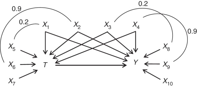
Simulated causal structure consisting of a dichotomous treatment (T), 6 binary covariates (X₁, X₃, X₅, X₆, X₈, and X₉), 4 standard-normal covariates (X₂, X₄, X₇, and X₁₀), and a continuous outcome (Y). The arrows represent causal effects. Each arc represents a correlation between the covariates, and the number above each arc represents the correlation coefficient.

In equation 3, we used the same parameter values for α₁ through α₇ as were used by Setoguchi et al. (18) and Lee et al. (19). We then simulated the outcome for each individual from a normal distribution with a mean of E[Y|X_i] (equation 3) and standard deviation of 1. Although binary outcomes are more common in pharmacoepidemiology, we chose to simulate a continuous outcome to simplify the analysis and to avoid issues with the noncollapsibility of the odds ratio (22). Because the PS models the relationship between covariates and treatment, we do not believe that the interpretation of the results when comparing various PS estimation methods will be substantially affected by using a continuous instead of a binary outcome.

As in the simulation structure used by Setoguchi et al. (18) and Lee et al. (19), correlations were induced between some of the covariates to be more reflective of practical settings (Figure 1). Lee et al. (23) provide a description and code for how these correlations were induced.

In each simulated study, we estimated the PS using logistic regression, bCART, and the CBPS. The logistic and CBPS models included only main effects for each of the covariates X₁–X₁₀ to reflect practical situations in which the true functional relations between covariates and treatment are unknown. For bCART, we used a maximum of 50,000 iterations with an iteration stopping point that minimized the mean of the Kolmogorov-Smirnov test statistic. We used 2 different parameter settings for the interaction depth. Because the scenarios in this simulation involve, at most, 2-way interactions, we used boosted classification and regression trees with an interaction depth of 2 (bCART2). In practice, the optimal interaction depth is unknown. Therefore, we also followed the recommendation of McCaffrey et al. (10), using boosted classification and regression trees with an interaction depth of 4 (bCART4). The bCART models were implemented using the twang package within the R statistical programming environment (24).

We implemented the PSs using both SMR weighting and inverse probability of treatment weighting (IPTW). For SMR weighting, weights were defined as 1 for individuals receiving treatment and PS / (1 − PS) (i.e., the odds of receiving treatment) for those not assigned to treatment. For IPTW, weights were defined as the inverse of the PS for individuals receiving treatment and 1 / (1 − PS) for those not receiving treatment. Because there is no treatment-effect heterogeneity built into the simulation structure, the average treatment effect in the treated and the average treatment effect in the population are equivalent. Therefore, both SMR weighting and IPTW should result in similar effect estimates when the PS is correctly specified. For each set of weights, we estimated the treatment effect using a weighted least squares regression of Y on T. We calculated the bias, defined as the expected value of the difference between the effect estimate and the true effect, by taking the mean of this difference over all simulation runs. The mean squared error (MSE) was calculated by taking the mean of the squared bias over all simulation runs. To evaluate precision, we estimated the standard error using the empirical standard deviation of the distribution of the treatment effect estimates across all simulation runs. We evaluated covariate balance by calculating the average standardized absolute mean difference (ASAMD) of the covariates across treatment groups. Because the data are simulated and the true PSs are known, we directly evaluated the mean prediction error for each PS model by calculating the absolute difference between the predicted PS and the true PS for each individual and then taking the mean of these differences across the entire population.

Empirical example: GLP-1 agonists versus sulfonylureas

We evaluated the performance of the described PS models using a 20% random sample of linked Medicare parts A (hospital), B (outpatient), and D (pharmacy) data. This sample included Medicare beneficiaries with fee-for-service enrollment in all 3 plans for at least 1 month during the calendar year between 2007–2009 (25). We compared new users of any GLP-1 agonist with new users of sulfonylureas in reducing combined coronary heart disease, cardiovascular disease, and all-cause mortality. The defined outcome included diagnostic codes for nonfatal myocardial infarction, angina, coronary revascularization, peripheral arterial disease, heart failure, stroke, and all-cause mortality. Our design decisions arose from the goal of simply demonstrating the PS methods under study, rather than producing a definitive comparison of GLP-1 agonists versus sulfonylureas.

New users were defined as individuals who began taking a GLP-1 agonist or sulfonylurea after having no prescription for any GLP-1 agonist or sulfonylurea during a 6-month washout period (i.e., allowing both cohorts to be taking other antidiabetic treatments, including metformin). We included all individuals who were continuously enrolled in Medicare for at least 12 months prior to drug initiation. All demographic and clinical covariates were defined during the 12 months prior to drug initiation. Individuals who had dual initiation of both a GLP-1 agonist and a sulfonylurea on the same day were excluded. The logistic PS model and the CBPS model included main effects for each of the covariates listed in Table 1. For the bCART models, we included the same parameter conditions described previously. The estimated PSs were implemented using SMR weighting. Because the true PSs are unknown, we evaluated the predictive performance for each of the PS models by calculating the mean absolute difference between the predicted PS value and the observed treatment status for each individual using 5-fold cross-validation to avoid rewarding models that overfit the data.

Table 1.

Unadjusted Distribution and SMR-Weighted Differences of Covariates Across New Users of GLP-1 Agonists and Sulfonylureas Within the Medicare Population, 2007–2009

Baseline Covariate	Unadjusted Distribution, %		Absolute Standardized Difference After SMR Weightinga
	GLP-1 Agonists (n = 725)	Sulfonylureas (n = 35,886)	Logisticb	bCART2	bCART4	CBPSc
Mean age, years	72.6	76.8	0.004	0.025	0.025	0.000
Female sex	34.3	38.9	0.001	0.027	0.009	0.000
Race
White	86.3	76.3	0.001	0.017	0.009	0.000
Black	6.9	12.4	0.000	0.034	0.024	0.000
Hispanic	3.4	4.9	0.021	0.036	0.025	0.000
Asian	1.4	3.6	0.000	0.019	0.016	0.000
Other	1.4	1.9	0.001	0.034	0.026	0.000
Medications
ACE inhibitor	36.3	38.7	0.000	0.030	0.020	0.000
Angiotensin receptor blocker	20.1	14.2	0.000	0.030	0.028	0.000
Anticholesteremic	2.9	2.8	0.002	0.003	0.005	0.000
Antidepressant	32.1	26.7	0.002	0.031	0.025	0.000
β Blocker	40.4	45.7	0.001	0.029	0.018	0.000
β2 Agonist	11.6	10.7	0.000	0.008	0.014	0.000
Bile acid sequestrant	1.9	1.1	0.001	0.024	0.020	0.000
Calcium channel blocker	25.9	30.0	0.001	0.028	0.016	0.000
Cholesterol absorption inhibitor	6.6	4.0	0.001	0.029	0.024	0.000
Fibrate	10.9	7.4	0.004	0.030	0.020	0.000
Glycoside	4.0	8.5	0.003	0.027	0.007	0.000
Loop diuretic	33.0	29.3	0.004	0.029	0.023	0.000
Metformin	59.7	50.7	0.002	0.024	0.016	0.000
Niacin	3.4	1.4	0.001	0.035	0.056	0.000
Nonloop diuretic	44.1	41.8	0.003	0.013	0.004	0.000
Progestin	0.3	1.3	0.000	0.041	0.029	0.000
Statin	64.7	56.3	0.001	0.032	0.023	0.000
Thiazolidinedione	28.6	16.3	0.004	0.019	0.023	0.000
Tests
Blood test	6.1	4.7	0.001	0.025	0.009	0.000
Electrocardiography	41.1	42.4	0.001	0.009	0.005	0.000
Lipid panel	77.9	63.1	0.001	0.034	0.028	0.000
Diagnoses
Cardiovascular heart failure	21.2	26.3	0.002	0.032	0.023	0.000
COPD	20.3	21.0	0.001	0.006	0.005	0.000
Depression	16.1	15.8	0.002	0.023	0.014	0.000
Diabetic complication	66.9	62.8	0.004	0.013	0.011	0.000
Gastrointestinal disorder	1.0	0.7	0.004	0.025	0.024	0.000
Infection	44.8	45.2	0.002	0.018	0.013	0.000
Nephropathy	9.8	6.3	0.002	0.016	0.020	0.000
Neuropathy	26.6	15.2	0.005	0.027	0.028	0.000
Retinopathy	20.0	12.2	0.005	0.026	0.025	0.000

Abbreviations: ACE, angiotensin-converting enzyme; bCART2, boosted classification and regression trees with interaction depth of 2; bCART4, boosted classification and regression trees with interaction depth of 4; CBPS, covariate-balancing propensity score; COPD, chronic obstructive pulmonary disease; GLP-1, glucagonlike peptide-1; SMR, standardized mortality ratio.

^a For binary covariates, we calculated the absolute standardized difference, not the absolute standardized percent differences.

^b Logistic model with main effects only.

^c CBPS with main effects only.

The effect of initiating GLP-1 agonists versus sulfonylureas in the weighted pseudopopulation was estimated using Cox proportional hazards models. Individuals were censored if they lost any part of Medicare coverage during follow-up or switched to or augmented treatment with the comparator drug during follow-up (i.e., as-treated analysis).

RESULTS

Simulation study

We present results for the simulation studies in Figures 2 and 3. Results are also provided in Web Tables 1–4, available at http://aje.oxfordjournals.org/. Figures 2 and 3 show that the CBPS performed best in terms of covariate balance for each of the scenarios. When treatment assignment was simulated using a logistic model, the ASAMDs for the CBPS model ranged from approximately 0.014 to 0.028 when PSs were implemented using SMR weighting and from 0.013 to 0.025 when PSs were implemented using IPTW (Figure 2). In these scenarios, the bCART models generally resulted in the greatest imbalance in the covariates. For example, the ASAMDs for the bCART2 model ranged from approximately 0.063 to 0.070 for SMR weighting and 0.091 to 0.108 for IPTW (Figure 2). Similar patterns were observed when treatment assignment was simulated using a probit model (Figure 3).

Figure 2.

Simulation results when treatment assignment was simulated using a logistic model. Propensity scores were implemented using standardized mortality ratio weighting in plots A, C, E, and G. Propensity scores were implemented using inverse probability treatment weighting in plots B, D, F, and H. The logistic and covariate-balancing propensity score (CBPS) models contained only main effects for each of the covariates. Scenario A, additivity and linearity; scenario B, mild nonlinearity; scenario C, moderate nonlinearity; scenario D, mild nonadditivity; scenario E, mild nonadditivity and nonlinearity; scenario F, moderate nonadditivity; scenario G, moderate nonadditivity and nonlinearity. ASAMD, average standardized absolute mean difference; bCART2, boosted classification and regression trees with interaction depth of 2; bCART4, boosted classification and regression trees with interaction depth of 4; MSE, mean squared error.

Figure 3.

Simulation results when treatment assignment was simulated using a probit model. Propensity scores were implemented using standardized mortality ratio weighting in plots A, C, E, and G. Propensity scores were implemented using inverse probability treatment weighting in plots B, D, F, and H. The logistic and covariate-balancing propensity score (CBPS) models contained only main effects for each of the covariates. Scenario A, additivity and linearity; scenario B, mild nonlinearity; scenario C, moderate nonlinearity; scenario D, mild nonadditivity; scenario E, mild nonadditivity and nonlinearity; scenario F, moderate nonadditivity; and scenario G, moderate nonadditivity and nonlinearity. ASAMD, average standardized absolute mean difference; bCART2, boosted classification and regression trees with interaction depth of 2; bCART4, boosted classification and regression trees with interaction depth of 4; MSE, mean squared error.

The CBPS model was the most consistent in terms of reducing both the bias and MSE in the estimated treatment effects. Figure 2 shows that the CBPS resulted in the lowest percent bias in 4 of the 7 scenarios for SMR weighting (scenarios B, D, E, and F), with percent bias ranging from 0.1% to 2.4%, and in 3 of the 7 scenarios for IPTW (scenarios C, F, and G), with percent bias ranging from 0.6% to 3.2%.

Figure 2 further shows that the CBPS resulted in the lowest MSE in 4 of the 7 scenarios when PSs were implemented using SMR weighting (scenarios A, B, C, and G), with the MSE ranging from 0.056 to 0.081, and in all 7 scenarios when PSs were implemented using IPTW, with the MSE ranging from 0.05 to 0.07 (Figure 2). Both the logistic regression and bCART models were less consistent in reducing the percent bias and MSE and were more sensitive to the method of weighting. Similar patterns were observed for scenarios in which the true PS followed a probit model (Figure 3).

In terms of predictive performance, Figure 2 shows that the bCART PS models were more stable across the 7 scenarios, with the mean prediction errors ranging from 0.075 to 0.086 for bCART2 and 0.085 to 0.091 for bCART4. The CBPS model generally resulted in a slightly higher prediction error than the logistic model, with the mean prediction errors ranging from approximately 0.04 to 0.18 for both SMR weighting and IPTW. Similar patterns were again observed when treatment assignment was simulated using a probit model (Figure 3).

To better understand the correspondence between the prediction of treatment assignment and covariate balance on the one hand and bias and MSE on the other, we aggregated the results from each of the simulations and plotted the percent bias and MSE against the ASAMD and mean prediction error (Figure 4). The ASAMD had a significant positive correlation with both percent bias (r = 0.82, P < 0.001) and MSE (r = 0.48, P < 0.001). The mean prediction error was not strongly related to bias (r = 0.13, P = 0.14) or MSE (r = −0.03, P = 0.78).

Figure 4.

Plotting covariate balance (average standardized absolute mean difference (ASAMD)) and mean prediction error against the percent bias in A and B and the mean squared error (MSE) in C and D. Plots include aggregated results from each of the simulations. The solid line in each plot represents the least squares regression line.

Empirical example: GLP-1 agonists versus sulfonylureas

Results for the empirical study comparing new users of GLP-1 agonists with new users of sulfonylureas are shown in Tables 1 and 2. In Table 1, we present the distribution of each of the covariates across treatment groups and standardized differences after SMR weighting. In Table 2, we present the estimated hazard ratios, standard errors, 95% confidence intervals, and overall covariate balance.

Table 2.

Comparing GLP-1 Agonists Versus Sulfonylureas on Time to Cardiovascular Event or All-Cause Mortality Within the Medicare Population, 2007–2009

Propensity Score Model	Hazard Ratio	Standard Error	95% CI	ASAMD	Prediction Errora
Unadjusted	0.719	0.102	0.589, 0.879	0.133
Logisticb	0.762	0.138	0.581, 0.999	0.002	0.038
bCART2	0.766	0.139	0.584, 1.005	0.025	0.038
bCART4	0.782	0.140	0.595, 1.029	0.020	0.037
CBPSc	0.763	0.138	0.582, 1.001	0.000	0.038

Abbreviations: ASAMD, average standardized absolute mean difference; bCART2, boosted classification and regression trees with interaction depth of 2; bCART4, boosted classification and regression trees with interaction depth of 4; CBPS, covariate-balancing propensity score; CI, confidence interval; GLP-1, glucagon-like peptide-1.

^a Prediction error was estimated by calculating the absolute difference between the predicted propensity score and observed treatment status using 5-fold cross-validation.

^b Logistic model with main effects only.

^c CBPS with main effects only.

For this example, each of the PS estimation methods resulted in covariates being approximately balanced across treatment groups. Although the differences were small, the CBPS model resulted in the best covariate balance (ASAMD < 0.000), followed by the logistic model (ASAMD = 0.002) and the bCART models (for bCART4, ASAMD = 0.02; for bCART2, ASAMD = 0.025).

The estimated treatment effect and precision were similar for each of the PS methods. Both the logistic and CBPS models resulted in a hazard ratio of approximately 0.76 with a standard error of 0.14. The bCART2 and bCART4 models resulted in hazard ratios of approximately 0.77 and 0.78, respectively, with a standard error of 0.14 for both models. Each of the models also resulted in similar performance in terms of the estimated prediction error (Table 2).

DISCUSSION

In this study, we used simulations and an empirical example to examine the performance of the CBPS relative to logistic regression and bCART when estimating PSs in situations where the logistic model assumptions are misspecified. For the scenarios assessed in the simulation, the CBPS method outperformed the other methods in terms of covariate balance. Although the CBPS model resulted in the lowest ASAMD for each scenario, no single method performed best in all scenarios in terms of bias in the estimated treatment effect. Many measures of covariate balance, including the ASAMD, do not take into account the strength of a particular variable's confounding. Further, the simulation structure reflects practical settings in which confounders induce bias in both directions. This can result in confounding bias canceling, even when covariates are not balanced across treatment groups. Therefore, the reduction in ASAMD did not always correspond with the greatest reduction in bias, although there was a strong correlation between the 2, and the CBPS generally performed well in terms of reduced bias compared with the logistic and bCART models.

We chose a simulation structure for treatment assignment that has been used in a number of previous studies (18, 19, 21, 26) and was originally constructed to include parameter values and covariate ranges that reflect those in pharmacoepidemiologic studies (18). As with any simulation, however, the observed results are specific to the scenarios considered, and one should avoid generalizing results to settings that have not been evaluated. Further, when the PS model is misspecified, results can be sensitive to the method of PS implementation, as illustrated in this study. Therefore, the observed results are specific not only to the causal scenarios assessed, but also to the methods of implementation that were considered in this study (SMR weighting and IPTW).

In the empirical example, the initial imbalance was modest (ASAMD = 0.13), and it was possible to balance all of the covariates well, regardless of the PS estimation method used. This may be due to the proper implementation of study design (e.g., active comparator, new user design and other restriction criteria) and the fact that covariates were primarily dichotomous. In settings with greater initial imbalance on important confounders, including continuous ones, larger performance differences may emerge. Small differences in percent bias due to model misspecification may well be outweighed by other biases (e.g., residual, information, measurement, misclassification, etc.), which cannot be addressed through PS models. This result supports the notion that, in pharmacoepidemiology and large database research, the greatest gains in the validity of effect estimates are likely achieved through state-of-the art study design rather than during the analytical phase (27).

Previous studies have shown that improving the predictive performance of a PS model through variable selection (e.g., including instrumental variables) does not necessarily correspond with improved confounding control (6–8). Results from this study showed that even when PS models controlled for the same set of covariates, there was not a strong correspondence between improved prediction of treatment assignment and improved confounding control.

By incorporating balance into the estimation process, the CBPS method does not approach PS parameter estimation with the objective of minimizing prediction error. In theory, incorporating covariate balance into PS estimation can provide a more robust method for estimating PSs in terms of covariate balance and bias. Researchers could improve covariate balance by refitting the logistic model using different functional forms of the covariates. In pharmacoepidemiology and large database research, however, refitting the logistic PS model until an acceptable degree of balance is achieved can be difficult. Because the CBPS estimates parameters in a way that minimizes covariate imbalance directly rather than minimizing prediction error, the CBPS can help to simplify the process of achieving covariate balance by avoiding the iterative process of refitting the logistic PS model. In principle, the CBPS can balance not only covariate means (as demonstrated in this paper), but also other distributional characteristics (15).

Similar to other parametric PS models, the CBPS method does not address variable selection. Ideally, one would estimate PSs that balance only risk factors for the outcome (7). Therefore, regardless of the PS estimation method used, we stress the importance of using study design and subject matter expertise to gain an understanding of the underlying causal structure before performing PS analysis (28). Within the CBPS and generalized method of moments framework, one could potentially improve bias reduction by placing more weight on balancing covariates with strong effects on the outcome. More research is needed in the area of automated weight/variable selection, as well as implementation of weights within the CBPS method.

It is unlikely that any single PS estimation method is optimal in every setting. More work is needed to better understand the performance of bCART and the CBPS over a wide variety of parameter constellations common to pharmacoepidemiology. We conclude that logistic regression with balance checks to assess model specification is a viable PS estimation method, but the CBPS seems to be a promising alternative.

REFERENCES

- 1.Rosenbaum PR, Rubin DB. The central role of the propensity score in observational studies for causal effects. Biometrika. 1983;70(1):41–55. [Google Scholar]
- 2.D'Agostino RB., Jr Tutorial in biostatistics: propensity score methods for bias reduction in the comparison of a treatment to a non-randomized control group. Stat Med. 1998;17(19):2265–2281. doi: 10.1002/(sici)1097-0258(19981015)17:19<2265::aid-sim918>3.0.co;2-b. [DOI] [PubMed] [Google Scholar]
- 3.Rosenbaum PR. Model-based direct adjustment. J Am Stat Assoc. 1987;82(398):387–394. [Google Scholar]
- 4.Robins JM. Association, causation, and marginal structural models. Synthese. 1999;121(1-2):151–179. [Google Scholar]
- 5.Rubin DB. On principles for modeling propensity scores in medical research. Pharmacoepidemiol Drug Saf. 2004;13(12):855–857. doi: 10.1002/pds.968. [DOI] [PubMed] [Google Scholar]
- 6.Westreich D, Cole SR, Funk MJ, et al. The role of the c-statistic in variable selection for propensity score models. Pharmacoepidemiol Drug Saf. 2011;20(3):317–320. doi: 10.1002/pds.2074. [DOI] [PMC free article] [PubMed] [Google Scholar]
- 7.Brookhart MA, Schneeweiss S, Rothman KJ, et al. Variable selection for propensity score models. Am J Epidemiol. 2006;163(12):1149–1156. doi: 10.1093/aje/kwj149. [DOI] [PMC free article] [PubMed] [Google Scholar]
- 8.Myers JA, Rassen JA, Gagne JJ, et al. Effects of adjusting for instrumental variables on bias and precision of effect estimates. Am J Epidemiol. 2011;174(11):1213–1222. doi: 10.1093/aje/kwr364. [DOI] [PMC free article] [PubMed] [Google Scholar]
- 9.Austin PC. Balance diagnostics for comparing the distribution of baseline covariates between treatment groups in propensity-score matched samples. Stat Med. 2009;28(25):3083–107. doi: 10.1002/sim.3697. [DOI] [PMC free article] [PubMed] [Google Scholar]
- 10.McCaffrey DF, Ridgeway G, Morral AR. Propensity score estimation with boosted regression for evaluating causal effects in observational studies. Psychol Methods. 2004;9(4):403–425. doi: 10.1037/1082-989X.9.4.403. [DOI] [PubMed] [Google Scholar]
- 11.Imai K, King G, Stuart EA. Misunderstandings between experimentalists and observationalists about causal inference. J R Stat Soc A. 2008;171(2):481–502. [Google Scholar]
- 12.Cepeda MS, Boston R, Farrar JT, et al. Comparison of logistic regression versus propensity score when the number of events is low and there are multiple confounders. Am J Epidemiol. 2003;158(3):280–287. doi: 10.1093/aje/kwg115. [DOI] [PubMed] [Google Scholar]
- 13.Stürmer T, Joshi M, Glynn RJ, et al. A review of the application of propensity score methods yielded increasing use, advantages in specific settings, but not substantially different estimates compared with conventional multivariable methods. J Clin Epidemiol. 2006;59(5):437–447. [Google Scholar]
- 14.Austin PC. An introduction to propensity score methods for reducing the effects of confounding in observational studies. Multivariate Behav Res. 2011;46(3):399–424. doi: 10.1080/00273171.2011.568786. [DOI] [PMC free article] [PubMed] [Google Scholar]
- 15.Imai K, Ratkovic M. Covariate balancing propensity score. J R Stat Soc B. 2014;76(1):243–263. [Google Scholar]
- 16.Graham BS, Campos de Xavier Pinto C, Egel D. Inverse probability tilting for moment condition models with missing data. Rev Econ Stud. 2012;79(3):1053–1079. [Google Scholar]
- 17.Hainmueller J. Entropy balancing for causal effects: a multivariate reweighting method to produce balanced samples in observational studies. Polit Anal. 2012;20(1):25–46. [Google Scholar]
- 18.Setoguchi S, Schneeweiss S, Brookhart MA, et al. Evaluating uses of data mining techniques in propensity score estimation: a simulation study. Pharmacoepidemiol Drug Saf. 2008;17(6):546–555. doi: 10.1002/pds.1555. [DOI] [PMC free article] [PubMed] [Google Scholar]
- 19.Lee BK, Lessler J, Stuart EA. Improving propensity score weighting using machine learning. Stat Med. 2010;29(3):337–346. doi: 10.1002/sim.3782. [DOI] [PMC free article] [PubMed] [Google Scholar]
- 20.Westreich D, Lessler J, Funk MJ. Propensity score estimation: neural networks, support vector machines, decision trees (CART), and meta-classifiers as alternatives to logistic regression. J Clin Epidemiol. 2010;63(8):826–833. doi: 10.1016/j.jclinepi.2009.11.020. [DOI] [PMC free article] [PubMed] [Google Scholar]
- 21.Austin PC. Using ensemble-based methods for directly estimating causal effects: an investigation of tree-based G-computation. Multivariate Behav Res. 2012;47(1):115–135. doi: 10.1080/00273171.2012.640600. [DOI] [PMC free article] [PubMed] [Google Scholar]
- 22.Greenland S, Pearl J, Robins JM. Confounding and collapsibility in causal inference. Stat Sci. 1999;14(1):29–46. [Google Scholar]
- 23.Lee BK, Lessler J, Stuart EA. Weight trimming and propensity score weighting. PLoS One. 2011;6(3):e18174. doi: 10.1371/journal.pone.0018174. [DOI] [PMC free article] [PubMed] [Google Scholar]
- 24.Ridgeway G, McCaffrey DF, Morral AR. Twang: Toolkit for Weighting and Analysis of Nonequivalent Groups. 2006. R Package Version 1.0-1. [Google Scholar]
- 25.United States renal data system. http://www.usrds.org/research.aspx . Published November 10, 1998. Updated May 23, 2014. Accessed May 28, 2014.
- 26.Leacy FP, Stuart EA. On the joint use of propensity and prognostic scores in estimation of the average treatment effect on the treated: a simulation study. Stat Med. doi: 10.1002/sim.6030. [published online ahead of print October 22, 2013]. ( doi:10.1002/sim.6030) [DOI] [PMC free article] [PubMed] [Google Scholar]
- 27.Stürmer T, Jonsson Funk M, Poole C, et al. Nonexperimental comparative effectiveness research using linked healthcare databases. Epidemiology. 2011;22(3):298–301. doi: 10.1097/EDE.0b013e318212640c. [DOI] [PMC free article] [PubMed] [Google Scholar]
- 28.Robins JM. Data, design, and background knowledge in etiologic inference. Epidemiology. 2001;12(3):313–320. doi: 10.1097/00001648-200105000-00011. [DOI] [PubMed] [Google Scholar]
Associated Data
This section collects any data citations, data availability statements, or supplementary materials included in this article.