

Abstract
The regional availability of oxygen in brain tissue is traditionally inferred from the magnitude of cerebral blood flow (CBF) and the concentration of oxygen in arterial blood. Measurements of CBF are therefore widely used in the localization of neuronal response to stimulation and in the evaluation of patients suspected of acute ischemic stroke or flow-limiting carotid stenosis. It was recently demonstrated that capillary transit time heterogeneity (CTH) limits maximum oxygen extraction fraction (OEFmax) that can be achieved for a given CBF. Here we present a statistical approach for determining CTH, mean transit time (MTT), and CBF using dynamic susceptibility contrast magnetic resonance imaging (DSC-MRI). Using numerical simulations, we demonstrate that CTH, MTT, and OEFmax can be estimated with low bias and variance across a wide range of microvascular flow patterns, even at modest signal-to-noise ratios. Mean transit time estimated by singular value decomposition (SVD) deconvolution, however, is confounded by CTH. The proposed technique readily identifies malperfused tissue in acute stroke patients and appears to highlight information not detected by the standard SVD technique. We speculate that this technique permits the non-invasive detection of tissue with impaired oxygen delivery in neurologic disorders such as acute ischemic stroke and Alzheimer's disease during routine diagnostic imaging.
Keywords: brain ischemia, imaging, kinetic modeling, mathematical modeling, MRI, neuroradiology
Introduction
Normal brain function requires a continuous supply of oxygen to meet the metabolic demands of neuroglial activity. The regional availability of oxygen in brain tissue is traditionally inferred from the magnitude of cerebral blood flow (CBF) and the concentration of oxygen in arterial blood. Cerebral blood flow is sensitive to regional levels of neuronal activity—known as neurovascular coupling—and methods to detect changes in CBF therefore provide powerful means of mapping brain function.
In disease, measurements of CBF are widely used in the evaluation of patients suspected having acute ischemic stroke or stenoocclusive carotid artery disease. The extent of CBF reduction below the ischemic threshold is thought to predict the development of permanent infarction in acute stroke,1 while the CBF response to well-defined vasodilator responses is used in the assessment of carotid artery disease severity.2
The microscopic distribution of CBF in brain tissue is rarely considered in the study of the pathogenesis of brain disorders. We recently demonstrated that the heterogeneity of capillary transit times affect oxygen extraction efficacy in tissue.3 By extending the classic flow-diffusion equation, we showed that the capillary blood mean transit time (MTT) and capillary transit time heterogeneity (CTH) combined determines the maximum oxygen extraction fraction (OEFmax) that can be achieved for a given tissue oxygen tension. In a series of recent papers, we review the putative effects of elevated CTH as a result of changes in capillary morphology in Alzheimer's disease,4 acute ischemic stroke,5 tumors,6 and subarachnoid hemorrhage.7 These reviews suggest that elevated CTH may reduce tissue oxygen availability, and thereby add to the propagation of tissue damage in these diseases. To study these hypotheses further, it is necessary to develop robust techniques for reliable estimation the MTT, CTH, and OEFmax. Such methods might reveal important information about the extent to which cerebral metabolism is limited by CBF, by the inability to homogenize capillary flows (so-called capillary dysfunction), or both.3
The heterogeneity of erythrocyte velocities along individual brain capillaries can be studied by direct microscopy in animal models.8, 9, 10 In humans, tracking of the passage of bolus-injected intravascular contrast agent by either computerized tomography or dynamic susceptibility contrast magnetic resonance imaging (DSC-MRI) can be used to indirectly quantify the retention of plasma in the cerebral microvasculature. The relative CBF and the tissue residue function, which denotes the proportion of contrast agent that remains in the vasculature at time t after it was injected as a narrow pulse, can be determined by deconvolving the tissue contrast concentration time curve with that of an artery.11 The residue function, in turn, is directly related to the distribution of vascular transit times, h(t), and hence to CTH.12 Owing to the inherent signal-to-noise constraints of computerized tomography and DSC-MRI, however, the use of model-free approaches may be suboptimal because of the unphysiological oscillations in the estimated residue function,13 which would propagate to its derivative and thereby CTH. While the regularization steps of model-free deconvolution approaches11, 13 may stabilize CBF estimates,14, 15, 16 they are not optimized to detect salient features of the residue function. This has led to the development of deconvolution approaches that instead use flexible, yet realistic, parametrized models to describe tissue residue in the deconvolution step.16, 17
We show that the expectation–maximization (EM) and Levenberg–Marquardt steps of an existing parametric approach17 can be explicitly calculated to allow simple and efficient computation of CTH and oxygen extraction capacity (OEFmax) in addition to the traditional ‘macroscopic' perfusion markers such as CBF and MTT. We assess the performance of the algorithm across a wide range of physiologic hemodynamic conditions,3 and evaluate its robustness to low signal-to-noise ratio (SNR) as well as bolus delay, and compare with model-free approaches.11, 13 Finally, we illustrate key similarities and differences between the new and the traditional perfusion maps in patients with acute ischemic stroke.
Theory
Tracer kinetic model
We assume that for a given tissue voxel, an intravascular tracer is delivered to the capillary bed with a characteristic arterial blood concentration denoted where t denotes time. Using indicator-dilution theory, the concentration of tracer in the capillaries at time  is proportional to the convolution of the arterial supply with the residue function, which represents the fraction of tracer still present in the capillaries at time t.
 |
where the constant κ depends on the hematocrit in the arterioles and capillaries, and the density of brain tissue, but is assumed constant in this paper.18
We adopt a gamma distribution for the capillary transit times3, 17, 19 to permit parametric estimation of the residue function.
 |
The gamma distribution has been used previously in studies of the dependence between CMRO2 and CBF.19 To accommodate any delay in tracer delivery to the capillaries relative to the site of arterial input function (AIF) measurement, an additional parameter is included in the model to permit shifts in the AIF timing, i.e., Ca(t)→Ca(t−δ).
Parameter estimation
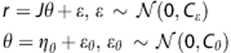
For measurements of the contrast concentration over time, we assume the nonlinear observation model
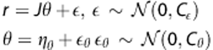
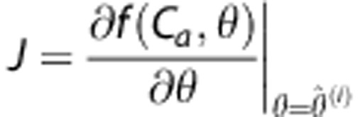
where f denotes the right hand side in equation (1), and θ represents the unknown parameter θ=(CBF,α,β,δ). We assume that the observation error ɛ follows a zero mean Gaussian distribution with covariance Cɛ. The parameter vector is also assumed to be stochastic with mean ηθ and covariance matrix Cθ. Parameter estimation can be performed from a frequentist point of view using the marginal distribution p(y) of y=(y1,…,yN). Owing to the unobserved stochastic elements in equation (4), EM is a natural way to estimate the free parameters.20 In the following, we use an EM-type algorithm based on a commonly applied linear expansion around a current estimate of the random effect,21, 22, 23 which still permits prior distributions on θ.17, 21 In contrast to previous methods, we develop an explicit equation for exact maximization in the M-step. A detailed description is provided in Appendix A. In brief, we use a Taylor expansion of the nonlinear function in equation (3) using the Jacobian.
 |
This leads to a linear model for the residual 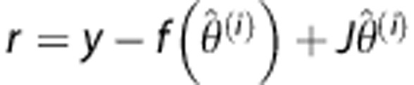 where y denotes the tissue concentration curve.
 |
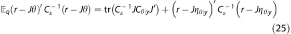
Parameter estimates can then be obtained by iteratively computing the posterior mean and covariance, ηθ|y and Cθ|y (see Appendix), and an exact expression of the variance.
 |
Materials and Methods
Calculating Oxygen Extraction Capacity
The relations between capillary transit times and OEFmax are described in detail in study by Jespersen and Østergaard.3 OEFmax is defined as
 |
where h(τ) is the capillary transit time distribution (equation (2)) and Q is the oxygen extraction along a single capillary with transit time τ. Further details of the computation of Q are presented in the Appendix.
Specifying the Prior Mean and Covariance
Computationally efficient estimates of CBF and MTT can be obtained using singular value decomposition (SVD).24 Although these estimates are known to be biased,13, 17 they may provide feasible first approximations, and are therefore used to center the prior. Delay is estimated as the time T-max to the maximum of the non-parametric estimate of the residue function.25 For the prior, we assume that the residue function is exponential by setting α=1 in equation (2), which implies β=MTT.
Acknowledging the inaccuracy of non-parametric estimates, the quality of the fit using the estimates of the EM algorithm is monitored by a relative root mean square error measure, i.e.,
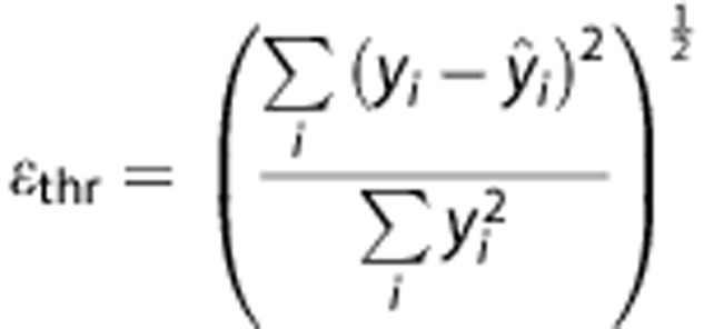 |
where yi represents data point i, and  the corresponding estimated value. If the squared error criterion exceeds a preset value for the final EM estimates (ɛthr>0.03), we reset the prior mean of CBF and δ to the current estimates while α is set to α=1 and β=MTT. The EM procedure is then repeated. This approach works well here, although we forego direct optimization of ɛthr.
For the prior covariance of the parameters, i.e., Cθ, we use a diagonal matrix, which reflects typical relative magnitudes of the corresponding parameters. Specifically, we set Cθ=diag(0.1,1,1,10). As in the study by Mouridsen et al,17 we model parameters on a log-scale, and the variances in Cθ therefore apply to the log-transformed parameters. We examine robustness to misspecification of Cθ below, see the section ‘Digital Phantom Images'.
Simulations
Concentration time curves were generated equation (1), and subsequently transformed to MRI signal. Specifically, the AIF was simulated using a gamma-variate function,26
 |
with a=1, t0=10, b=3, and c=1.5 to generate an arterial concentration time curve with a shape and amplitude typical of standard clinical injection schemes.13, 17, 18, 24 Simulations were performed for CBV=4%.27 Signal curves were then generated using
with S(0)=100 and echo time=50 ms and where r2 is the transverse relaxivity. The constant κr2 was calibrated as in the studies by Wu et al, Mouridsen et al, and Calamante et al13, 17, 18 to produce signal drops typically observed in DSC data, such that a CBF of 60 ml per 100 g/minute and a CBV of 4% produces a 40% signal drop relative to the baseline as is typical for normal gray matter. For the AIF, κr2 was fixed to produce a 60% signal drop relative to baseline.13
Gaussian noise with zero mean was added to the signal curves equation (11) to produce specific baseline SNRs. The sampling rate was fixed at repetition time=1.5 seconds and an acquisition time of 99 seconds including a 10.5 seconds baseline was simulated.
Digital Phantom Images
The capillary transit time distribution h(τ) in equation (8) is completely specified by its mean, MTT=αβ and s.d.  . To assess whether MTT and CTH can be independently estimated, we created a digital phantom where these quantities vary across a grid. This mimics Figure 4A in study by Jespersen and Østergaard,3 which illustrates the dependence of OEFmax on the transit time distribution, although in the present study, we consider a broader range of MTT and CTH values. Each phantom consists of 7 × 7 squares, all of which correspond to a certain combination of MTT and CTH. Each square is subdivided into 14 × 14 voxels, all with identical MTT and CTH, but different noise realizations. Mean transit time varied from 2 seconds to 20 seconds along the x-direction and CTH from 2 seconds to 20 seconds along the y-direction. Squares were separated by two voxels. The true values of CTH and OEFmax are shown in the left column in Figure 1 and the true MTT values are displayed in the left column in Figure 3.
Figure 4.

Standard deviation (A) and bias (B) of the mean transit time (MTT) for the different models as a function of the signal-to-noise ratio (SNR). Mean transit time values were fixed at 30 seconds if the estimates exceeded this value. The bias for the parametric model continues to decrease with increasing SNR, whereas for singular value decomposition (SVD), there is no considerable improvement beyond and SNR of ∼60. oSVD, oscillatory SVD; sSVD, standard SVD.
Figure 1.

The phantoms in the left column represent the true capillary transit time heterogeneity (CTH) and maximum oxygen extraction fraction (OEFmax) values of the digital phantom. Mean transit time (MTT) and CTH values vary from 2 to 20 seconds along columns (MTT) and rows (CTH). The center and right column shows estimated values at signal-to-noise ratio (SNR)=100 (center) and SNR=20 (right column). The unit of the color bar is seconds for the CTH maps, while the OEFmax maps are dimensionless. Little bias is observed at SNR=100. At SNR=20, the CTH estimates exhibit minor bias for very high MTT, while OEFmax is well estimated except for combinations of very high flow and CTH.
Figure 3.

Mean transit time (MTT) maps computed by the proposed parametric, standard singular value decomposition (sSVD), and oscillatory SVD (oSVD) methods for signal-to-noise ratio (SNR)=20 and SNR=100. The true values are shown in the left column. Mean transit time is well estimated at SNR=100 with the parametric model, whereas both the SVD methods demonstrate pronounced bias, even at high SNR. The SVD estimates are apparently confounded by capillary transit time heterogeneity (CTH) (which varies across rows), whereas the parametric technique appears able to produce independent estimates of MTT and CTH.
Phantoms were generated with SNRs between 10 and 500. We also simulated arterial tracer arrival delays by introducing a time difference between the start of the AIF and the start of the tissue curves C(t). Delays were varied between 0 seconds and 10 seconds.
While the non-parametric SVD provides adequate initial estimates of hemodynamic parameters to serve as centers of the prior distribution, the prior covariance is more difficult to determine. We examine the robustness to misspecification by varying the scales of CBF and the transport function parameter α, which together represent overall flow (CBF) and transit time distribution (α). We consider an alternative covariance matrix  where the variance of CBF has been scaled up by a factor of 10 and the variance of α has been scaled down by the same factor. This effectively interchanges the scales of CBF and α. We also evaluate algorithm performance in the digital phantom for covariance matrices with intermediate scale changes using as prior covariance matrix
 |
and calculate the mean square error in the phantom for values of ζ ranging from ζ=0 to ζ=1 with increments of 1/20. We compare results of the present algorithm with exact maximization to the iterative Fisher Scoring scheme in the study by Mouridsen et al.17
Patient Data
Magnetic resonance imaging from seven patients with anterior circulation strokes were studied to compare the hemodynamic maps produced with the proposed algorithm to the standard SVD methods. Patient data were obtained as part of the I-Know stroke imaging project (www.i-know-stroke.eu). The multicenter protocol was approved by the respective national Ethics Committees and informed consent was obtained before patient enrollment. Standard DSC-MRI was performed on a Siemens Avanto 1.5, a Siemens Sonata 1.5, or a Philips Intera 1.5 scanner. Dynamic echo planar imaging (echo time=50 ms, repetition time=1,500 ms, field-of-view=24 cm, matrix 128 × 128, slice thickness 5 mm) was performed during intravenous injection of Gadolinium-based contrast (0.1 mmol/kg) at rate of 5 ml/second, followed by 30 mL of physiologic saline injected at the same rate. Follow-up fluid-attenuated inversion recovery (FLAIR) images were acquired after 1 week or 1 month to assess the extent of the final infarct.
Image Processing
Analysis of phantom images as well as patient data was performed with the Penguin perfusion software developed at our institution (www.cfin.au.dk/software/penguin). In the clinical data, an AIF was identified semi-automatically by an expert radiologist. Parametric estimation of hemodynamic parameter maps was performed with the presets described above. Standard SVD was applied with a threshold of 0.2,24 and with oscillatory SVD (oSVD),13 the oscillation index was set to 0.095. With the SVD methods, delay was estimated as the time to maximum of the residue function (T-max).25
Quantification of Parameter Estimation Performance
Within fields in the digital phantom, we summarize the ability to estimate each marker using bias between true and estimated values and s.d. It is known that the mean square error can be decomposed into the sum of the squared bias and variance, but we consider the components individually to characterize accuracy as well as precision. Specifically, variance, bias and mean square error are calculated as
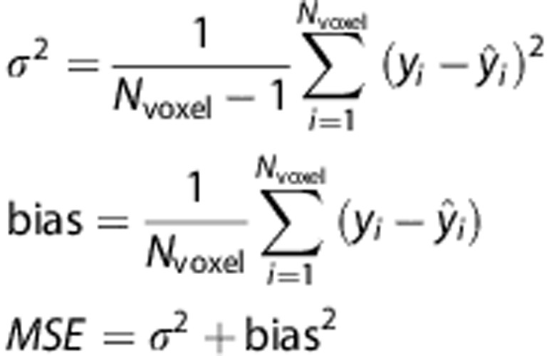 |
where Nvoxel is the number of voxels in a square, yi is the true value, and  is the estimated value. To summarize the performance over the entire phantom we use the average bias and s.d. across the 49 fields.
Results
Estimation of Capillary Transit Time Heterogeneity and Maximum Oxygen Extraction Fraction at specific Signal-to-Noise Ratios
Figure 1 shows OEFmax and CTH estimates in the digital phantom at SNR=100 and SNR=20. The true values are displayed in the phantom in the left column. At SNR=100 (center column), estimates of CTH and OEFmax are in good agreement with the true values, demonstrating no appreciable bias and little within-field intensity variation.
At SNR=20, the CTH estimates show low bias and little variation among squares in the horizontal direction, indicating that CTH can be estimated independently of MTT even in conditions with considerable image noise. As expected, within-square variance increases at the lower SNR, but CTH differences remain discernible across MTT levels. As shown by the lower panels, the variance and bias of the OEFmax estimates behaved in a similar fashion, except for some bias (overestimation) of OEFmax in cases of very high flow (low MTT) and high transit time heterogeneity.
In Figure 2, the bias and s.d. of the OEFmax and CTH parameters are plotted for SNR ranging from 10 to 500. Both parameters exhibit fast convergence about improvements in the SNR in terms of both bias and s.d., and it is observed that bias dominates over s.d., albeit the quantities are relatively small. The higher bias at low SNR results from cases with very high heterogeneity and flow as seen in Figure 1. This corresponds to the residue function rapidly dropping from its maximum to a level close to zero, which is maintained over a long time period to account for the high heterogeneity. At low SNR, this subtle characteristic may be difficult to identify.
Figure 2.

Standard deviation (alternating dot and dashed line) and bias (dashed line) of the capillary transit time heterogeneity (CTH) (cross) and maximum oxygen extraction fraction (OEFmax) (open diamonds) parameters as a function of signal-to-noise ratio (SNR). The units of CTH are in seconds.
Estimation of Mean Transit Time at Specific Signal-to-Noise Ratios
While CTH and OEFmax estimates are specific to our technique, MTT estimates can be compared with standard SVD (sSVD) and oSVD. Figure 3 shows MTT estimates by the parametric model and by the two SVD techniques at SNR=100 (top panels) and SNR=20 (bottom panels). Comparing with the true MTT values shown to the far left, we note that at SNR=100, the parametric model exhibits no discernible bias and exhibits low within-field variation. Combined with the similar results for CTH in Figure 1, this ascertains the algorithm's ability to provide independent estimates of MTT and CTH. In comparison, sSVD and oSVD both demonstrate substantial bias in MTT estimates. When CTH is low, as in the lower rows of the phantom, this bias is low, but it increases for moderate CTH (middle rows) and for high CTH, the MTT estimates appear close to uniform across columns, indicating little agreement with the varying true MTT values in the phantom across the columns.
At SNR=20, the parametric procedure demonstrates a slight bias in MTT for mid-range values of CTH. For high CTH values, the bias is more pronounced for low MTT values (upper left corner), and as for the CTH estimates discussed above we attribute the bias to the intricate behavior of the residue function for this particular combination of CTH and MTT. Meanwhile, the SVD methods display substantial bias even at very low CTH.
We note that the residue function is exponential along the diagonal from the lower left to the upper right corner. Both SVD techniques appear to give reasonable estimates of MTT along this direction, which is consistent with previous results13, 24 in this special case.
General Signal-to-Noise Ratio Sensitivity of Mean Transit Time
To compare the performance of the perfusion algorithms across a wider range of conditions, Figure 4 summarizes the concordance between the estimated and the true MTT values in terms of s.d. (Figure 4A) and bias (Figure 4B). Both quantities are observed to decrease rapidly as SNR increases for the parametric algorithm. For the SVD methods, only the s.d. decreases as SNR improves. The bias is observed to be virtually independent of SNR, leveling out at ∼6 seconds (oSVD) and 7 seconds (sSVD), respectively. This is in contrast to bias for the parametric method, which is below 0.5 seconds at high SNR. This confirms the visual assessment of Figure 3.
Sensitivity to Tracer Delay from the Site of Arterial Input Function Measurement
Figures 5A and 5B shows s.d. and bias for all modalities for tracer delays between 0 and 10 seconds for fixed SNR=50. Cerebral blood flow estimates are in arbitrary units.
Figure 5.

Standard deviation (A) and bias (B) as a function of delay using the parametric model (blue), standard singular value decomposition (sSVD) (green), and oscillatory SVD (oSVD) (red). The delay is given in seconds. CBF, cerebral blood flow; CTH, capillary transit time heterogeneity; MTT, mean transit time; OEF, maximum oxygen extraction fraction.
For all comparable parameters (MTT, CBF, delay), the performance on bias and s.d. is better with the parametric approach than SVD, with the exception of the CBF s.d. Notably, the bias in MTT is 2 to 3 seconds higher with SVD than the parametric approach, and the bias in SVD delay estimates averages ∼3 seconds, with the parametric delay maps below one. Although some dependence on tracer delay is observed in all curves, there appears to be no discernible systematic trends, and the order across modalities and techniques in terms of their bias and s.d. appears mostly unaffected by delay changes.
Parametric Model: Robustness about Prior Covariance
In Figure 6, ζ=0 corresponds to the prior covariance matrix used in this study and ζ=1 represents an alternative covariance matrix where the scales of CBF and α have changed by a factor of 10. Figure 6 shows the effect of scale changes in the prior covariance matrix on, respectively, the previously described approach17 and the present. We see that the exact optimization approach is more robust to prior covariance misspecification than the iterative procedure, where a sudden increase in bias is observed across all modalities around ζ=0.5. The s.d. is observed (Figure 6A)) to vary for both the iterative and exact step algorithms, but on much smaller scale compared with the bias in Figure 6B).
Figure 6.

The effect of scale changes in the prior covariance matrix on s.d. (A) and bias (B). The exact maximization (blue curves) derived in this study provides robustness to scale changes whereas a sudden increase in bias of parameter estimates is observed with the iterative approach (red curves). CTH, capillary transit time heterogeneity; MTT, mean transit time.
Patient Data
Clinical data for the seven stroke patients, labeled A to G, are presented in Table 1. Figure 7 shows perfusion maps from the parametric procedure and the SVD techniques, as well as follow-up FLAIR images showing the subsequent lesion. To visualize differences in CTH and MTT maps, we also generated maps of their ratio, CTH/MTT, which is the coefficient of variation for the transit time distribution (CoV).
Table 1. Clinical characteristics of the patients.
| ID | Age | Gender | NIHSS | Occlusion | Time from onset (hours) | Recanalization at 2 days | Time of follow-up (days) |
|---|---|---|---|---|---|---|---|
| A | 47 | F | 11 | M1 | 5.35 | Partial | 15 |
| B | 62 | M | 5 | Intracranial ICA | 6.05 | None | 29 |
| C | 70 | M | 14 | M2 | 1.55 | None | 14 |
| D | 74 | M | 14 | MCA distal | 0.22 | Minimal | 20 |
| E | 74 | F | 4 | M1 | 1.23 | Complete | 7 |
| F | 87 | F | NA | MCA distal | NA | NA | 56 |
| G | 89 | F | 10 | M2 | 01.02 | Partial | 8 |
ICA, internal carotid artery; MCA, middle cerebral artery with branches M1 and M2; NIHSS, national institutes of health stroke scale.
Figure 7.

Perfusion markers for a set of clinically acquired stroke data. Variation for the transit time distribution (CoV) denotes the coefficient of variation, and is a measure of the dissimilarity between the parametric capillary transit time heterogeneity (CTH) and mean transit time (MTT) maps. In general, the perfusion lesions appear more distinct on the parametric MTT and CTH maps compared with singular value decomposition (SVD)-based MTT. We also note the large difference in lesion volumes between the parametric and SVD techniques in patients E, F, and G, where the parametric maps appear in better correspondence with follow-up T2 fluid-attenuated inversion recovery shown in the bottom row. OEF, maximum oxygen extraction fraction; oSVD, oscillatory SVD; sSVD, standard SVD.
In patient A, all metrics demonstrate a large hypoperfused region consistent with the patient's neurologic deficits (national institutes of health stroke scale=11). Parametric MTT and CTH images, however, seem to distinguish the hypoperfused tissue more clearly from surrounding, unaffected tissue. Although MTT and CTH are both elevated, their ratio as indicated in the CoV map, display a more homogeneous distribution than the MTT and CTH maps within the lesion area. Note that CTH and MTT appear ‘matched', with CoV values just above unity, in unaffected tissue.
In patient B, the lesion appears much less clear on SVD MTT maps, compared with maps of parametric MTT, OEFmax, and CTH. Notably, the anterior boundary of the lesion is difficult to identify on SVD images, possibly because of the image noise. The CoV map indicates that the MTT increase is matched by an increase in CTH. We notice, however, a marked decrease in CTH relative to MTT (lower CoV) in a smaller subregion in which follow-up images show subsequent infarction (see arrow).
Scattered noise in SVD-based perfusion maps is common, as shown in patient C, in the hemisphere contralateral to the hypoperfused tissue. Low raw data contrast-to-noise ratios (typically 3 to 5 in this patient) result in negative values in the concentration time curves of single voxels, and therefore, fast oscillating residue functions and inaccurate CBF estimates after SVD deconvolution. The parametric model fits to realistic and flexible residue curves that, by construction, cannot become negative, and may therefore still fit meaningful values from the shape of the bolus passage. This finding is consistent with our phantom simulations, in which low SNR gave rise to a significant overestimation of MTT for the SVD methods, see Figure 3. In this patient, the MTT prolongation is matched by a CTH increase.
In patient D, there is less consistency in the lesion estimate across SVD and parametric images, with parametric MTT displaying a high-intensity volume consistent with the final outcome, whereas the SVD MTT maps may suggest less grading of intensities. Capillary transit time heterogeneity appears to be elevated throughout the lesion. According to the simulation results above, the lesion patterns on SVD MTT maps could represent bias due to elevated transit time heterogeneity. Again, only the region with low CoV showed signs of infarction on follow-up FLAIR.
The apparent overestimation of perfusion lesions with the SVD methods is more evident in patient E, in which parametric MTT and CTH are only slightly elevated. The modest degree of tissue involvement is consistent with the moderate neurologic deficits, national institutes of health stroke scale=4. In this patient, parametric and SVD methods all indicated a large bolus delay within an area that corresponds to the SVD MTT lesion (data not shown). This phenomenon may suggest that neurologic function was preserved because of the efficient collateral blood supply in the MCA territory. The CoV map indicates a minor CTH decrease relative to MTT.
In contrast to patient E, patients F and G do not show any hypoperfusion on oSVD MTT, whereas lesions are clearly visible on parametric MTT, OEFmax and CTH. The lesion is visible on the sSVD MTT map for patient G, but less so in patient F. In both cases, the lesions observed in the parametric perfusion images are consistent with the 1-month follow-up FLAIR lesions. Inspection of the underlying signal curves revealed that short data acquisition time, resulting in truncated signal curves in hypoperfused tissues, may have contributed to the low sensitivity of the oSVD MTT map. The parametric model maps and standard SVD MTT map seemed unaffected by the truncation phenomenon in these patients. Low CoV again appears to accurately match the 1-month follow-up lesions.
In addition to the visual assessment, Supplementary Figure 1 displays the summary of a quantitative analysis. We used the consensus outlines of end infarct as delineated on the follow-up FLAIR images by four experienced readers (with consensus defined as two or more ‘votes' for each voxel) to identify actual tissue outcome. For each patient and hemodynamic marker, we computed the average and s.d. of image intensities in the acute images in the location corresponding to the final infarct. We also computed analogous values in a region around, but not including, the end lesions. This region was established as a 10-voxel dilation of the end infarct (discounting CSF and non-brain voxels). This analysis was not limited to the image slices shown in Figure 7. After the arrangement in Figure 7, the Supplementary Figure 1 displays pairs of values in the end-lesion and perilesion areas for each patient. All values are relative to contralateral white matter. The top three bar plots confirm that the proposed method provides better contrast between regions that ultimately infarct, compared with the surrounding tissue. We also note that OEFmax values are consistently higher in tissue that proceeds to infarction, and we observe that s.d. values appear relatively small compared with the mean values. Furthermore, as is seen in the bottom graph, this numerical analysis confirms that CoV is typically lower in the tissue proceeding to infarct.
Discussion
We have modeled the combined effect of CBF, and its microscopic distribution across the capillary bed, on the tracer retention observed in DSC-MRI. We developed a statistical technique for estimating the resulting parameters, CTH and MTT, and determined the derived oxygen extraction capacity, OEFmax, based on raw data typical of clinical DSC-MRI. This method extends existing techniques for the estimation of ‘macroscopic' perfusion indices—CBF, CBV, and MTT—to take the effects of CTH on the retention of tracer in tissue into account. Our simulation results demonstrate low bias and variance in MTT, CTH, and OEFmax estimates across a wide range of residue functions, even in data with poor SNR. Importantly, these estimates are also relatively insensitive to delays between the site of AIF measurement and region of interest, which is a common concern in acute stroke imaging. We have examined how MTT estimates made by sSVD and oSVD reflect the underlying MTT and CTH values. We found that the MTT values retrieved by these widely used techniques fail to reflect the underlying MTT in cases where CTH is high (Figure 3), even at low noise levels (SNR=100).
We examined cases of acute ischemic stroke to confirm our simulation results, namely the characterization of tracer retention in brain tissue by CTH and MTT reveals information not detected by conventional MTT maps alone. This analysis revealed cases in which patients with severe neurologic symptoms showed no lesions on oSVD perfusion maps. In these cases, the new parameter maps revealed lesions at the location of subsequent infarction. We also observed cases in which lesions in parametric maps appeared more congruent with the neurologic deficits of the patients than those of the oSVD and SVD techniques. These preliminary findings are consistent with earlier reports, which suggested that abnormal capillary heterogeneity provides prognostic information not available by conventional MTT maps.
Mean transit time and CTH are hypothesized to co-determine net oxygen extraction in tissue.3 Elevated CTH reduces the oxygen extraction efficacy OEFmax, whereas increased MTT has competing effects in that it increases OEFmax on one hand, while reducing total oxygen supply (CBF falls rapidly as MTT increases) on the other. This phenomenon is particularly important in acute stroke, where a thromboembolic event is likely to reduce CBF and thus cause an increase in MTT, while changes in blood rheology or capillary morphology (as a result of cerebrovascular risk factors or prolonged ischemia), are likely to affect CTH.7 We observed clear differences between MTT and CTH maps, as illustrated with the CoV images. A low CTH relative to MTT appears to signal infarct across all patient cases with a specificity seemingly exceeding MTT alone (patients B, D). With the accuracy of the technique demonstrated in our simulations this is encouraging, but further investigations in larger patient cohorts are necessary to support this finding.
Our simulations clearly demonstrate shortcomings in the SVD techniques in accounting for more subtle characteristics of the residue function such as CTH. While so-called model-free deconvolution, (such as SVD) suggests that any residue function shape can be retrieved because the ‘range' of possible functions is not limited a priori, in practice, the range is indeed limited, and a model is indeed suggested albeit implicitly. For the SVD approach, residue functions are constructed as linear combinations of the columns of the inverse of the AIF (in matrix form).3 Therefore, a ‘model' is indirectly established that determines the range of possible residue functions (specifically functions in the column space of the inverse AIF matrix). Critically, random measurement error in the AIF will translate to systematic bias in the possible residue functions, which can be formed with this model, and may therefore prevent the detection of subtle characteristics in the microvascular flow. While noise reduction approaches will reduce oscillations by effectively reducing the complexity of the basis functions, they cannot overcome the inherent inadequacy of the model, and may further reduce the sensitivity to intricate residue function characteristics. Moreover, the residue function for a particular voxel is formed by weighing the basis functions by the values of the concentration curve, which are also offset by noise. In sum, SVD is not model independent, but rather establishes a model based entirely on the measured AIF, thereby inheriting its noise components, and uses as model coefficients the error prone measured concentrations. We therefore believe that the approach suggested in this study offers both a more realistic and flexible model and a more favorable noise reduction than the SVD by (a) directly addressing the residue functions (instead of the measured AIF), (b) fitting a realistic and noise-free model of the tracer retention to the data, rather than a model derived from noisy observations of an AIF typically measured relatively far from the voxel-of-interest and (c) avoiding restricting the physiologic plausibility of the residue functions in the regularization approach.
Limitations of the Study
The dimensions of a typical capillary bed in the human brain are typically of the order of hundreds of micrometers—far smaller than the typical image voxel of raw perfusion MRI images (typically 2.5 × 2.5 × 5 mm). Therefore, the fitted residue function represents the average retention across hundreds of (possibly interconnected) capillary beds. The extent to which the transit time characteristics of capillary beds vary in space (across neighboring capillary bed or regionally) and time (The model is typically fitted to 20 to 30 seconds of perfusion-weighted imaging data) remains poorly understood. Microscopy studies that examine the temporal and spatial dynamics of capillary flow patterns are therefore needed to address to which extent the values of CTH determined by this approach are typical of individual capillary bed. For example, large spatial and temporal variability in the MTT of individual capillary beds could be interpreted as a condition of high CTH by our method even if the capillary flow patterns of each capillary bed were homogenously distributed. We expect the capillary flow patterns of individual capillary beds to be very heterogeneous,3 but also note that redistribution of blood flow on the microscopic scale at a time scale of seconds by vasomotion may affect its estimates.
Perfusion-weighted imaging is sensitive to the susceptibility contrast generated by Gd-based contrast agent, which distributes only in plasma. The transit time characteristics determined by our method are therefore those of plasma rather than full blood, and, more specifically, those of plasma in the vascular compartments that the perfusion-weighted imaging method is most sensitive to. In healthy brain capillaries, transit time heterogeneity for plasma is slightly smaller than that of blood, seemingly because blood cells fail to compartmentalize plasma completely during their passage through individual capillaries.28 In disease, capillary morphology is often severely disturbed, and one might therefore expect the capillary passage of erythrocytes to be more affected in disease conditions than that of plasma. Perfusion-weighted imaging is typically performed by gradient echo echo planar imaging, which is sensitive to contrast agent in primarily larger, non-capillary vessels, whereas spin echo echo planar imaging is relatively more sensitive to contrast agent in capillary-sized vessels.29, 30 The use of spin echo-based perfusion-weighted imaging may therefore provide data that are relatively specific to the retention of tracer in capillaries as opposed to in larger, downstream venules and veins. Meanwhile, gradient echo-based perfusion-weighted imaging data may provide higher sensitivity to heterogeneity of capillary flow patterns among (as opposed to within) capillary beds within an image voxel by being sensitive to the transit time distributions of downstream venules and veins. Finally, we note that susceptibility contrast mechanisms may differ according to the distribution of plasma and red blood cells in individual capillaries.31
The present work improves the estimation step of our earlier technique17 by deriving the exact maximum in the M-step of the EM algorithm. When combined with a reinitialization strategy in case of poor convergence, the algorithm performs substantially better than the iterative optimization method across all perfusion markers (Figure 6). The estimation scheme still depends on the accuracy of the first order approximation (equation (13)). The error introduced by ignoring the nonlinearity in equation (3) could be characterized32 by means of Monte Carlo simulations, but the accuracy of perfusion estimates demonstrated above suggests the linear approximation to be adequate, and any further gain would come at the cost of excessive computing time.
We have compared the performance of our approach to that of the traditional sSVD and oSVD. Several model independent methods for retrieving CBF and MTT have been suggested,15, 33, 34 along with flexible analytical algorithms.14, 16 However, the SVD-based techniques are the most widely used techniques, and it is beyond the scope of this study to perform a comparison with other approaches
The simulations in our work are based on a gamma distribution for the capillary transit times. This is in line with previous work17 and the gamma distribution has previously been applied in studies on the relation between CMRO2 and CBF.19 The choice of this more complex transit time model extends previous investigations on the estimation of hemodynamic parameters,13, 18, 24 in which only simple residue functions (exponential, box-car and linear) were considered. We note that these simple residue functions, while intuitively compelling, restrict the variability of MTT and CTH. The exponential function models the microvasculature as a well-mixed compartment, and corresponds to the gamma distribution with the constraint MTT=CTH. The box-car residue function models ‘plug' flow and occur only in the special case of CTH=0. The linear residue function, in turn, implies that  . This study instead addresses a broad range of capillary transit time distribution, such as those studied in Jespersen.3 The gamma distribution represents a wide range of microvascular flow patterns and has been used previously in related studies.19 Still, direct measurements of transit time distributions by microscopy in animal models or preoperatively in humans, or rigorous simulation models of capillary systems35 could be used to examine the appropriateness of this choice in the healthy and diseased brain.
Perspectives
In clinical stroke data, an interesting evaluation of the proposed methodology would be the assessment of correspondence between clinical manifestations (national institutes of health stroke scale score) and volume or level of hypoperfusion as estimated by MTT and CTH, as patient examples A and E indicate the current method may estimate perfusion deficits in better correspondence with clinical findings. An even more detailed assessment taking into account differences in eloquence across different brain regions could be obtained with so called voxel-level predictive algorithms.
Although the oxygen extraction capacity computed with the proposed technique represent the maximum amount affordable for particular levels of MTT and CTH, a direct comparison in clinical data with positron emission tomography could give additional important information on the performance of this method. This may be an option primarily in other diseases than acute stroke, as any time difference between MRI and positron emission tomography acquisitions may influence the interpretability of the results.
In a recent review, we demonstrated that tissue oxygen availability might be critically reduced in conditions in which CTH is elevated.7 We expect CTH to be elevated as a result of cerebrovascular risk factors that alter the morphology and function of capillaries, thereby preventing the normal regulation of capillary flow patterns. Under such conditions, additional increases in CTH (caused for example by altered blood viscosity after infections or dehydration) or minor CBF changes (hypotensive episodes or a minor thromboembolic event) may elicit critical reductions in tissue oxygenation and trigger neurologic symptoms.5 While such patients may present with symptoms of an acute stroke and display lesions on both diffusion and perfusion-weighted MRI, this hypothesis predicts that tissue oxygenation can be improved by reducing CTH, for example, by managing blood rheology via rehydration or reduction of leukocytosis by appropriate management of infections. In this way, some neuroprotection may be instigated before thrombolytic therapy, and in patients who are ineligible for recanalization therapy. Similarly, ischemia has been shown to result in deteriorating capillary flow patterns36 and widespread capillary constrictions,37, 38 possibly contributing to the metabolic derangement of periinfarct tissue. We therefore speculate that knowledge of CTH may improve our understanding of acute stroke pathophysiology and the future management of this condition.
Acknowledgments
The authors wish to thank their I-Know study collaborators J.-C. Baron, A. Alawneh (Cambridge), S. Pedraza, J. Puig (Girona), N. Nighoghossian, T.-H. Cho (Lyon), and S. Siemonsen, J. Fiehler (Hamburg) for providing patient examples to this study.
APPENDIX
Oxygen Extraction Fraction
To calculate the oxygen extraction fraction in equation (9), we compute the numerical solution to the ordinary differential equation (see study by Jespersen and Østergaard3 for details)
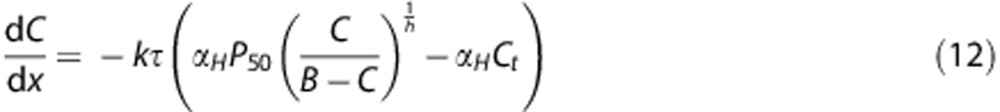 |
where k describes the capillary wall permeability to oxygen, C is the concentration of oxygen, and τ is the capillary transit time. Solving equation (9) for the oxygen concentration C immediately produces the oxygen extraction fraction, for a given transit time τ, as Q=1−C(1)/C(0.) The maximum oxygen extraction for a tissue voxel can then be calculated by equation (8) when the distribution of transit times is estimated. The remaining constants have been adopted from the study by Jespersen and Østergaard3 and are αH=3.1 × 10⁻⁵/mm Hg, B=0.1943 ml/mL, P50=26 mm Hg , and Ct=25 mm Hg. The rate constant k is set by requiring OEFmax=30% in normal-appearing white matter in the clinical stroke data included in this paper. The resulting value is found to be k=38/second.
Expectation–Maximization
In this appendix, we derive the exact expressions for the E- and M-step in the estimation algorithm described under ‘Theory'. Following Friston,20 we consider the first order expansion of f about a current estimate  of the random effect (equations (3), (4)),
 |
where
 |
For the residual  , where y denotes the tissue concentration curve, we have
 |
The marginal distribution of the data is
assuming that ɛ and ɛθ are independent on each other. Effectively, this is a special case of a statistical linear mixed model, where the second term in the covariance structure in equation (14) results from the random effects.39 However, to allow regularization of parameter estimates, we use a Bayesian approach where the hyperparameters  (ηθ, Cθ) of θ are given. An EM-type algorithm naturally applies to estimating the error covariance Cɛ and the posterior mean ηθ|y and covariance Cθ|y of θ.
 |
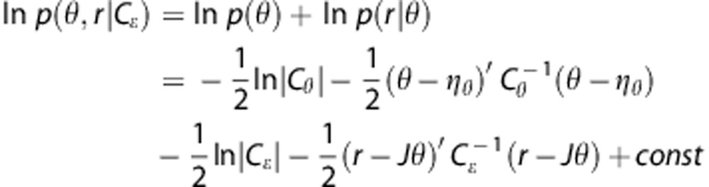
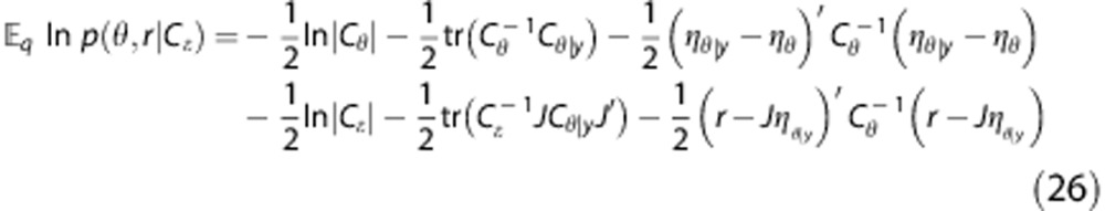
E-step. The joint density p(θ,r|Cɛ) in equation (15) can be written as
As both densities are Gaussian, we get
 |
The posterior density q(θ|y) is also Gaussian with parameters ηθ|y and Cθ|y given by
 |
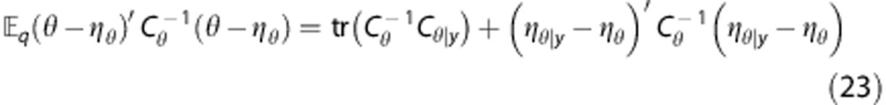
To calculate the mean of ln p(θ,r|Cɛ) when θ has the posterior density q, we use that the expectation of the quadratic form z′Az is
 |
Where A is a matrix,  z=μ and CoV(z)=Σ. Therefore, as under the posterior distribution we have
 |
it follows that
 |
Analogously
 |
which gives
 |
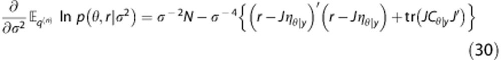
Therefore, the expression to be maximized about Cɛ in the M-step is
 |
M-step. To derive the exact optimization in the M-step, we first let Cɛ=σ2Q, where Q describes the structure (e.g., weighting) of co-variances, and calculate the partial derivative of equation (26). We note that
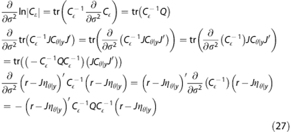 |
The first derivative of the expression in the M-step can then be written as
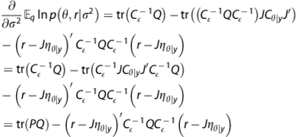 |
where
Now consider the case, where there is only a single variance component, i.e., Cɛ=σ2 I. In this case, equation (28) reduces to
 |
where N is the number of observations. The optimal value can now be found directly by setting the differential equal to zero, yielding
 |
As in study by Mouridsen et al,17 the expansion point, in equation (13) is reset using regularization with a Levenberg–Marquardt damping factor, by taking advantage of the equivalence of the EM-approach to estimating the posterior modes with a Newton algorithm maximizing the posterior density of θ, as pointed out in Friston.20
KM and MBH are co-applicants on a patent application based on the presented technique (EP 13185195.8). KM and MBH are shareholders in Combat Stroke. The remaining authors declare no conflict of interest.
Footnotes
Supplementary Information accompanies the paper on the Journal of Cerebral Blood Flow & Metabolism website (http://www.nature.com/jCBFm)
This study was supported by the Danish National Research Foundation (CFIN; KM, LØ, SNJ), the Danish Ministry of Science, Technology and Innovation's University Investment Grant (MINDLab; KM, MBH, LØ, SNJ), and the European Union's 6th Framework Program (I-Know; KM, LØ).
Supplementary Material
References
- Astrup J, Siesjo BK, Symon L. Thresholds in cerebral ischemia—the ischemic penumbra. Stroke. 1981;12:723–725. doi: 10.1161/01.str.12.6.723. [DOI] [PubMed] [Google Scholar]
- Powers WJ. Cerebral hemodynamics in ischemic cerebrovascular disease. Ann Neurol. 1991;29:231–240. doi: 10.1002/ana.410290302. [DOI] [PubMed] [Google Scholar]
- Jespersen SN, Østergaard L. The roles of cerebral blood flow, capillary transit time heterogeneity, and oxygen tension in brain oxygenation and metabolism. J Cereb Blood Flow Metab. 2012;32:264–277. doi: 10.1038/jcbfm.2011.153. [DOI] [PMC free article] [PubMed] [Google Scholar]
- Østergaard L, Aamand R, Gutierrez-Jimenez E, Ho Y-L, Blicher JU, Madsen SM, et al. The capillary dysfunction hypothesis of Alzheimer's disease. Neurobiol Aging. 2013;34:1018–1031. doi: 10.1016/j.neurobiolaging.2012.09.011. [DOI] [PubMed] [Google Scholar]
- Østergaard L, Jespersen SN, Mouridsen K, Mikkelsen IK, Jonsdottir K, Tietze A, et al. The role of the cerebral capillaries in acute ischemic stroke: the extended penumbra model. J Cereb Blood Flow Metab. 2013;33:635–648. doi: 10.1038/jcbfm.2013.18. [DOI] [PMC free article] [PubMed] [Google Scholar]
- Østergaard L, Tietze A, Nielsen T, Drasbek KR, Mouridsen K, Jespersen SN, et al. The relationship between tumor blood flow, angiogenesis, tumor hypoxia, and aerobic glycolysis. Cancer Res. 2013;73:5618–5624. doi: 10.1158/0008-5472.CAN-13-0964. [DOI] [PubMed] [Google Scholar]
- Østergaard L, Aamand R, Karabegovic S, Tietze A, Blicher JU, Mikkelsen IK, et al. The role of the microcirculation in delayed cerebral ischemia and chronic degenerative changes after subarachnoid hemorrhage. J Cereb Blood Flow Metab. 2013;33:1825–1837. doi: 10.1038/jcbfm.2013.173. [DOI] [PMC free article] [PubMed] [Google Scholar]
- Kleinfeld D, Mitra PP, Helmchen F, Denk W. Fluctuations and stimulus-induced changes in blood flow observed in individual capillaries in layers 2 through 4 of rat neocortex. Proc Natl Acad Sci USA. 1998;95:15741–15746. doi: 10.1073/pnas.95.26.15741. [DOI] [PMC free article] [PubMed] [Google Scholar]
- Stefanovic B, Hutchinson E, Yakovleva V, Schram V, Russell JT, Belluscio L, et al. Functional reactivity of cerebral capillaries. J Cereb Blood Flow Metab. 2008;28:961–972. doi: 10.1038/sj.jcbfm.9600590. [DOI] [PMC free article] [PubMed] [Google Scholar]
- Villringer A, Them A, Lindauer U, Einhaupl K, Dirnagl U. Capillary perfusion of the rat brain cortex. An in vivo confocal microscopy study. Circ Res. 1994;75:55–62. doi: 10.1161/01.res.75.1.55. [DOI] [PubMed] [Google Scholar]
- Østergaard L, Weisskoff RM, Chesler DA, Gyldensted C, Rosen BR. High resolution measurement of cerebral blood flow using intravascular tracer bolus passages. Part I: mathematical approach and statistical analysis. Magn Reson Med. 1996;36:715–725. doi: 10.1002/mrm.1910360510. [DOI] [PubMed] [Google Scholar]
- Østergaard L, Chesler DA, Weisskoff RM, Sorensen AG, Rosen BR. Modeling cerebral blood flow and flow heterogeneity from magnetic resonance residue data. J Cereb Blood Flow Metab. 1999;19:690–699. doi: 10.1097/00004647-199906000-00013. [DOI] [PubMed] [Google Scholar]
- Wu O, Østergaard L, Weisskoff RM, Benner T, Rosen BR, Sorensen aAG. Tracer arrival timing-insensitive technique for estimating flow in MR perfusion-weighted imaging using singular value decomposition with a block-circulant deconvolution matrix. Magn Reson Med. 2003;50:11. doi: 10.1002/mrm.10522. [DOI] [PubMed] [Google Scholar]
- Andersen IK, Have AS, Rasmussen CE, Hansson L, Marstrand JR, Larsson HB, et al. Perfusion Quantification Using Gaussian Process Deconvolution. Magn Res Med. 2002;48:351–361. doi: 10.1002/mrm.10213. [DOI] [PubMed] [Google Scholar]
- Calamante F, Gadian DG, Connelly A. Quantification of bolus-tracking MRI: improved characterization of the tissue residue function using Tikhonov regularization. Magn Reson Med. 2003;50:1237–1247. doi: 10.1002/mrm.10643. [DOI] [PubMed] [Google Scholar]
- Mehndiratta A, MacIntosh BJ, Crane DE, Payne SJ, Chappell MA. A control point interpolation method for the non-parametric quantification of cerebral haemodynamics from dynamic susceptibility contrast MRI. NeuroImage. 2013;64:560–570. doi: 10.1016/j.neuroimage.2012.08.083. [DOI] [PubMed] [Google Scholar]
- Mouridsen K, Friston K, Hjort N, Gyldensted L, Østergaard L, Kiebel S. Bayesian estimation of cerebral perfusion using a physiological model of microvasculature. NeuroImage. 2006;33:570–579. doi: 10.1016/j.neuroimage.2006.06.015. [DOI] [PubMed] [Google Scholar]
- Calamante F, Gadian DG, Connelly A. Delay and dispersion effects in dynamic susceptibility contrast MRI: simulations using singular value decomposition. Magn Res Med. 2000;44:466–473. doi: 10.1002/1522-2594(200009)44:3<466::aid-mrm18>3.0.co;2-m. [DOI] [PubMed] [Google Scholar]
- Buxton RB, Frank LR. A Model for the coupling between cerebral blood flow and oxygen metabolism during neural stimulation. J Cereb Blood Flow Metab. 1997;17:64–72. doi: 10.1097/00004647-199701000-00009. [DOI] [PubMed] [Google Scholar]
- Dempster AP, Laird NM, Rubin DB. Maximum likelihood from incomplete data via the EM algorithm. J Royal Stat Soc B. 1977;39:1–38. [Google Scholar]
- Friston KJ. Bayesian estimation of dynamical systems: an application to fMRI. NeuroImage. 2002;16:513–530. doi: 10.1006/nimg.2001.1044. [DOI] [PubMed] [Google Scholar]
- Lindstrom MJ, Bates DM. Newton-Raphson and EM algorithms for linear mixed-effects models for repeated-measures data. J Am Stat Assoc. 1988;83:1014–1022. [Google Scholar]
- Mentré F, Gomeni R. A Two-step iterative algorithm for estimation in nonlinear mixed-effect models with an evaluation in population pharmacokinetics. J Biopharm Stat. 1995;5:141–158. doi: 10.1080/10543409508835104. [DOI] [PubMed] [Google Scholar]
- Østergaard L, Weisskoff RM, Chesler DA, Gyldensted C, Rosen BR. High resolution measurement of cerebral blood flow using intravascular tracer bolus passages. Part I: mathematical approach and statistical analysis. Magn Res Med. 1996;36:715–725. doi: 10.1002/mrm.1910360510. [DOI] [PubMed] [Google Scholar]
- Calamante F, Christensen S, Desmond PM, Østergaard L, Davis SM, Connelly A. The physiological significance of the time-to-maximum (Tmax) parameter in perfusion MRI. Stroke. 2010;41:1169–1174. doi: 10.1161/STROKEAHA.110.580670. [DOI] [PubMed] [Google Scholar]
- Rausch M, Scheffler K, Rudin M, Radu EW. Analysis of input functions from different arterial branches with gamma variate functions and cluster analysis for quantitative blood volume measurements. Magn Res Imaging. 2000;18:1235–1243. doi: 10.1016/s0730-725x(00)00219-8. [DOI] [PubMed] [Google Scholar]
- Leenders KL, Perani D, Lammertsma AA, Heather JD, Buckingham P, Healy MJR, et al. Cerebral blood flow, blood volume and oxygen utilization. Normal values and effect of age. Brain. 1990;113:27–47. doi: 10.1093/brain/113.1.27. [DOI] [PubMed] [Google Scholar]
- Vogel J, Waschke KF, Kuschinsky W. Flow-independent heterogeneity of brain capillary plasma perfusion after blood exchange with a Newtonian fluid. Am J Physiol. 1997;272 (4 Pt 2:H1833–H1837. doi: 10.1152/ajpheart.1997.272.4.H1833. [DOI] [PubMed] [Google Scholar]
- Weisskoff RM, Zuo CS, Boxerman JL, Rosen BR. Microscopic susceptibility variation and transverse relaxation: theory and experiment. Magn Reson Med. 1994;31:601–610. doi: 10.1002/mrm.1910310605. [DOI] [PubMed] [Google Scholar]
- Kjolby BF, Ostergaard L, Kiselev VG. Theoretical model of intravascular paramagnetic tracers effect on tissue relaxation. Magn Reson Med. 2006;56:187–197. doi: 10.1002/mrm.20920. [DOI] [PubMed] [Google Scholar]
- Frohlich AF, Ostergaard L, Kiselev VG. Theory of susceptibility-induced transverse relaxation in the capillary network in the diffusion narrowing regime. Magn Reson Med. 2005;53:564–573. doi: 10.1002/mrm.20394. [DOI] [PubMed] [Google Scholar]
- Walker S. An EM algorithm for nonlinear random effects models. Biometrics. 1996;52:934–944. [Google Scholar]
- Grüner R, Taxt T. Iterative blind deconvolution in magnetic resonance brain perfusion imaging. Magn Reson Med. 2006;55:805–815. doi: 10.1002/mrm.20850. [DOI] [PubMed] [Google Scholar]
- Wirestam R, Ståhlberg F. Wavelet-based noise reduction for improved deconvolution of time-series data in dynamic susceptibility-contrast MRI. Magma. 2005;18:113–118. doi: 10.1007/s10334-005-0102-z. [DOI] [PubMed] [Google Scholar]
- Pries AR, Secomb TW. Comprehensive Physiology. John Wiley & Sons, Inc; 2011. Blood Flow in Microvascular Networks. [Google Scholar]
- Tomita Y, Tomita M, Schiszler I, Amano T, Tanahashi N, Kobari M, et al. Moment analysis of microflow histogram in focal ischemic lesion to evaluate microvascular derangement after small pial arterial occlusion in rats. J Cereb Blood Flow Metab. 2002;22:663–669. doi: 10.1097/00004647-200206000-00004. [DOI] [PubMed] [Google Scholar]
- Peppiatt CM, Howarth C, Mobbs P, Attwell D. Bidirectional control of CNS capillary diameter by pericytes. Nature. 2006;443:700–704. doi: 10.1038/nature05193. [DOI] [PMC free article] [PubMed] [Google Scholar]
- Yemisci M, Gursoy-Ozdemir Y, Vural A, Can A, Topalkara K, Dalkara T. Pericyte contraction induced by oxidative-nitrative stress impairs capillary reflow despite successful opening of an occluded cerebral artery. Nat Med. 2009;15:1031–1037. doi: 10.1038/nm.2022. [DOI] [PubMed] [Google Scholar]
- Laird NM, Ware JH. Random-effects models for longitudinal data. Biometrics. 1982;38:963–974. [PubMed] [Google Scholar]
Associated Data
This section collects any data citations, data availability statements, or supplementary materials included in this article.