

Abstract
We present a novel approach to the third order spectral analysis, commonly called bispectral analysis, of electroencephalographic (EEG) and magnetoencephalographic (MEG) data for studying cross-frequency functional brain connectivity. The main obstacle in estimating functional connectivity from EEG and MEG measurements lies in the signals being a largely unknown mixture of the activities of the underlying brain sources. This often constitutes a severe confounder and heavily affects the detection of brain source interactions. To overcome this problem, we previously developed metrics based on the properties of the imaginary part of coherency. Here, we generalize these properties from the linear to the nonlinear case. Specifically, we propose a metric based on an antisymmetric combination of cross-bispectra, which we demonstrate to be robust to mixing artifacts. Moreover, our metric provides complex-valued quantities that give the opportunity to study phase relationships between brain sources.
The effectiveness of the method is first demonstrated on simulated EEG data. The proposed approach shows a reduced sensitivity to mixing artifacts when compared with a traditional bispectral metric. It also exhibits a better performance in extracting phase relationships between sources than the imaginary part of cross-spectrum for delayed interactions. The method is then applied to real EEG data recorded during resting state. A cross-frequency interaction is observed between brain sources at 10 Hz and 20 Hz, i.e., for alpha and beta rhythms. This interaction is then projected from signal to source level by using a fit-based procedure. This approach highlights a 10–20 Hz dominant interaction localized in an occipito-parieto-central network.
Keywords: Functional connectivity, cross-frequency interactions, higher order spectral analysis, bispectrum, brain networks, volume conduction
1. Introduction
Electroencephalography (EEG) and Magnetoencephalography (MEG) are non invasive techniques which provide the opportunity to directly measure ongoing brain activity with very high temporal but relatively low spatial resolution. While in the past decades the main focus of EEG/MEG studies was on the analysis of event related potentials, i.e. the average brain response to a given stimulus, more recently the variability of brain activity has attracted many researchers. The recent interest in this field reflects the understanding that a mere localization of specific brain activities is far from sufficient to understand how the brain operates, but that it is necessary to study the brain as a network. In this framework, the analysis of brain rhythms has been recognized as a promising approach since coherent neuronal activity has been hypothesized to serve as a mechanism for neuronal communication (Fries, 2009; Gross et al., 2006; Miller et al., 2009; Tallon-Baudry et al., 1996; Womelsdorf and Fries, 2006).
The study of brain connectivity using noninvasive electrophysiological measurements like EEG or MEG also presents some problems which still need to be faced. Most notably, the fact that the data are a largely unknown mixture of the activities of the actual brain sources constitutes a severe confounder. For instance, two sensors can record from the same neural populations, opening the possibility for spurious interactions between sensors in the absence of true brain interactions. Though the problem of mixing artifact is well known (Nunez et al., 1997), it is increasingly acknowledged and studied not only for channel data (often referred to as volume conduction or field spread) (Srinivasan et al., 2007; Winter et al., 2007) but also at the source level, i.e., after source activities have been estimated from channel data using an inverse calculation (Schoffelen and Gross, 2009). Indeed, almost all the linear and nonlinear methods used to analyze multivariate data for neuroscientific applications (an excellent overview can be found in Pereda et al., 2005) are highly sensitive to mixing artifacts.
To overcome the problem of volume conduction it was suggested to exploit the fact that the propagation of electromagnetic fields is much faster than neural communication: while phase shifts between electric scalp potentials (EEG) or neuromagnetic fields (MEG) and the underlying source activity are too small to be observable (Stinstra and Peters, 1998), the temporal resolution of the data is still sufficient to capture phase shifts of neuronal signal propagation. This observation has been exploited in the imaginary part of coherency (ImCoh), a measure of brain connectivity which cannot be caused by mixtures of independent sources (Nolte et al., 2004). However, in the presence of interacting sources, the actual value still depends on how sources are mapped into sensors (Nolte et al., 2004) or on source space (Sekihara et al., 2011). This drawback was addressed for two sources using pairwise measures with the lagged phase coherence (Pascual-Marqui, 2007b; Pascual-Marqui et al., 2011) or with the weighted phase lag index (Vinck et al., 2011).
Nonlinear methods to estimate correlations between power addressing the issue of artifacts of volume conduction have also been recently suggested. In Brookes et al. (2012), the authors address the problem of field spread which generates spurious source space connectivity results. Using a seed based approach, the linear projection of the seed voxel is first regressed out from the signals at the test voxel and, then, power correlations are assessed both within and across multiple frequency bands. Similarly, in Hipp et al. (2012), sensor signals are orthogonalized before computing power envelope correlations at the same or different frequencies, thus removing signal components that share the same phase.
A noteworthy approach to the problem of volume conduction is proposed in Gómez-Herrero et al. (2008). Here, after an initial Principal Component Analysis (PCA), the authors propose to subtract a linear multivariate autoregressive model from sensor data to suppress all time-delayed correlations, with the idea that all neural interactions require a minimum delay. An Independent Component Analysis (ICA) is then applied to the residuals and the ICA mixing matrix is used to model the effects of volume conduction (see also Hyvärinen et al., 2010). This approach takes note of the fact that a direct application of ICA to the data would be a conceptual contradiction to the objective of the research, namely studying causality relationships between sources.
In this paper, we address the problem of mixing artifacts in relation to the use of nonlinear methods for studying cross-frequency phase-synchronization between neuronal populations. Specifically we refer to bispectral measures, which were developed and applied on EEG/MEG in abundance (Darvas et al., 2009a,b; Dumermuth et al., 1971; Helbig et al., 2006; Jirsa and Müller, 2013; Schwilden, 2006; Wang et al., 2007), and we examine the question of what information can be derived from such measures that estimates true functional connectivity between brain regions as opposed to mixing artifacts. Our new contribution is, essentially, the generalization to nonlinear methods of the concepts based on the imaginary part of coherency to solve the problem of volume conduction (Marzetti et al., 2008; Nolte et al., 2004, 2008, 2009). As will be shown below, for linear measures (e.g., cross-spectra), the imaginary part equals the antisymmetric part (apart from a factor ι, i.e., the imaginary unit) and the antisymmetry property is the more general principle from which measures robust to artifacts of volume conduction can be derived for second-order (linear) and for third-order (nonlinear) moments. In this way, antisymmetrized cross-bispectra can be used along with the imaginary part of cross-spectra for identifying phase-locked brain areas without being confounded by mixing artifacts, but with the important difference that the former reflects the presence of brain rhythms locked together at different frequencies, while the latter focuses on interactions at the same frequency. Moreover, the proposed approach has also the advantage of improving, for a certain class of interactions, a limitation of the imaginary part of the cross-spectrum, which cannot provide information about relative phases, i.e. the phase difference of the activities of two brain sources, in a way which is robust to artifacts of volume conduction. Indeed, the imaginary part of the cross-spectrum is itself a real and not a complex valued quantity, and real values do not contain information about relative phases. Hence, the dilemma of linear measures is the fact that possibly interesting quantities cannot be estimated in a way which is robust to artifacts of volume conduction. On the contrary, the antisymmetric part of third order moments (cross-bispectra) is itself complex and hence contains phase information which are not corrupted by noninteracting sources.
The paper is organized as follows. In the Material and methods section, we present the theory for cross-bispectral measures robust to mixing artifacts. Specifically, we first recall the basic principles of the imaginary part of cross-spectrum and, then, we introduce the antisymmetric part of the cross-bispectrum, discussing its properties with regards to mixing artifacts. We describe a strategy to project the interaction from channel to source level by using a fit-based procedure. We also discuss some examples of interpretation of the phase of cross-bispectral measures. In the Result section, we first analyze the performance of our method in a simulation study, where we apply it on simulated EEG data. We then describe an example of application of the method to real EEG data. Finally, the Discussion section provides remarks on the method features and on its ability to give an insight on cross-frequency functional connectivity.
2. Material and methods
2.1. Theory for cross-bispectral measures robust to mixing artifacts
2.1.1. Cross-spectra and mixing artifacts
We first recall some principles of second order statistical analysis in the frequency domain. The respective statistical moments, the elements of the cross-spectral matrix S, are defined as
| (1) |
where Xi(f) and Xj(f) are the Fourier coefficients of (eventually windowed) segments of data in channel i and channel j at frequency f, * denotes complex conjugation, and 〈·〉 denotes taking the expectation value, i.e. taking the hypothetical average over an infinite number of segments. Of course, the expectation value is unknown and will in general be estimated by a finite average over segments. Since S = S†, where (·)† denotes transpose and complex conjugation, S is an hermitian matrix. Complex coherency, C, is defined as the cross-spectrum normalized by power, i.e. the diagonal elements of it:
| (2) |
It was argued that the imaginary part of the coherency is a useful quantity to study brain interaction because it cannot be generated from a superposition of independent sources (Nolte et al., 2004). For later use we rederive this result assuming that the data have zero mean which, if not vanishing, has to be subtracted from the raw data. We now assume that all sources sk(f) are mapped instantaneously into channels as
| (3) |
with aik being real valued coefficients corresponding to the forward mapping of the kth source to the ith channel. Then the cross-spectrum can be written as
| (4) |
If we now assume that all sources are independent, the second term on the right hand side in the above equation vanishes because for k ≠ k′
| (5) |
Since the first term in (4) is real valued, a non-vanishing imaginary part of S must arise from interacting sources and can be used to study brain interactions. This applies equally to coherency where the cross-spectrum was normalized with the real valued power. Note, that the first term in (4) is not only real valued but also symmetric with respect to switching the channel indices i and j.
The relation between the antisymmetric part of S, , and the imaginary part of S follows immediately from the fact that S is hermitian, resulting in
| (6) |
where ι denotes the imaginary unit. The above relation (6) does not exist for higher order moments, and, as it will be seen below, it is the symmetry property which can be generalized to higher order statistical moments.
2.1.2. Bispectral analysis
Let Xi(f), Xj(f) and Xk(f) be the Fourier transforms of time series recorded by three EEG (or MEG) channels i, j, and k. The cross-bispectrum, which is essentially a measure of the quadratic phase coupling between signal components at frequencies f1, f2 and f1 + f2, is given by
| (7) |
where 〈·〉 represents the expectation value over a sufficiently large number of signal segments.
The cross-bispectrum and other bispectral measures, e.g., bicoherence (Nikias and Petropulu, 1993), have been widely used to detect and quantify the non-linear and non-gaussian properties of EEG/MEG signals (Dumermuth et al., 1971; Helbig et al., 2006; Schwilden, 2006; Wang et al., 2007), with a particular interest in sleep studies (Barnett et al., 1971; Bullock et al., 1997) and anaesthesia monitoring (Johansen and Sebel, 2000). Methods for nonlinear connectivity estimation based on bispectral analysis of EEG recordings have also been developed (e.g., Shils et al., 1996; Villa and Tetko, 2010). Almost all these methods, however, are highly sensitive to mixing artifacts, and spurious interactions might be detected when analyzing data. A solution is to first localize the sources of brain activity and, then, apply the bispectral analysis to source time courses (see for example Darvas et al., 2009b). However, the obtained results is in general only free of mixing artifacts if the inverse solution accurately separates all sources which is hardly ever the case.
Here, we introduce a new bispectral measure for sensor-level connectivity estimation which is robust to mixing artifacts. We do not replace the goal of a source-level analysis, since the interaction can further be projected onto brain space, but, in such way, the estimated interaction is not affected by the validity of the inverse method. In particular, we look at the part of the cross-bispectrum which is antisymmetric to the permutation of two channel indices, e.g., i and k in the following example1:
| (8) |
To see that the antisymmetrized cross-bispectrum of (8) cannot be generated from independent sources, we assume that all sources, sm(f), are independent and insert that into (7)
| (9) |
The ‘coupling terms’ contain expressions of the form where not all indices m, n, p are identical, i.e. at least one of the indices is different from the other two. If, e.g., this index is the first one, m, and all sources are independent, this term vanishes
| (10) |
and likewise for any other of the indices.
Hence, for independent sources we get
| (11) |
which is totally symmetric with respect to the three channel indices. From this it follows that an antisymmetric combination with respect to any pair of indices must vanish for independent sources. Below we will restrict ourselves mainly to the case f1 = f2, namely we will focus on cross-frequency interactions involving one frequency, f1 = f2 = f, and its double, f1 + f2 = 2f. In this case only one antisymmetric combination is relevant, namely antisymmetrization of the first and last index as given in (8). Since Bijk(f1, f2) = Bjik(f1, f2) the other two possible antisymmetric combination are either redundant, B[i|j|k](f1, f2) = Bj[ik](f1, f2), or vanish, B[ij]k(f1, f2) = 0. Note that in general B[i|j|k](f1, f2) is complex and allows to reconstruct phases also from quantities which are robust to mixing artifacts. This is in sharp contrast to second order statistics: when restricting to the imaginary (or antisymmetric) part of cross-spectrum, any information on phases is lost.
The above symmetry property required the vanishing of coupling terms for independent sources. We emphasize that this only holds up to third order statistical moments. For three (source) indices and if two indices are equal, the third index is either different from both and the corresponding (vanishing) mean can be factored out, or all indices are equal and the contribution to the cross-bispectrum is totally symmetric. For fourth or higher order, the coupling terms in general do not vanish even if the sources are independent. E.g. for m ≠ k, for independent sources sm and sk, and for f2 = −f1 one gets
| (12) |
for non-vanishing signal power.
2.1.3. Normalization
It has been shown (Nikias and Petropulu, 1993; Van Ness, 1966) that, for sufficiently large sample size, the estimation of the cross-bispectrum by using conventional methods provides unbiased estimates with asymptotic variance:
| (13) |
where δf1f2 is the Kronecker delta and is the power spectrum of the ith process and similarly for j and k. This means that, in general, the variance of the bispectral estimate increases with signal power and, if the averaging is insufficient, large peaks may appear in the cross-bispectrum because it is highly variable and not because there is a significant phase coupling at that frequency pair. A normalization is, then, required in order to avoid improper interpretations. Here, we divide the cross-bispectrum by the standard deviation of its estimate, as follows:
| (14) |
with the standard deviation being computed as the conventional standard error of the mean, i.e.,
| (15) |
where P denotes the number of segments into which the signals were divided. As an alternative, since it is known from (13) that the variances of the real and imaginary parts of the cross-bispectrum are asymptotically equal, a pooled estimator of the standard deviation can be calculated as , and used in the denominator of (14). The adopted normalization allows to suppress statistically meaningless estimates, thus assessing the robustness of obtained results. Similarly, the normalization of the antisymmetric part of the cross-bispectrum is achieved by dividing both the real and the imaginary part of B[i|j|k] by the standard deviation of their estimates, as follows:
| (16) |
2.1.4. Fit of the interaction
Once a statistically significant antisymmetric part of the cross-bispectrum has been detected and, thus, an interaction has been isolated at sensor level, the signal can be projected onto the brain space using a specific interaction model. In the following, we describe a model consisting of two arbitrarily distributed interacting sources.
Given an N-channel EEG (or MEG) recording, if we denote by s1(f) and s2(f) the source activities in the frequency domain and by ai and bi, i = 1…N, respectively, their real-valued topographies, i.e. Xi(f) = ais1(f) + bis2(f), then, according to (7) and (8), the antisymmetric part of the cross-bispectrum for each triplet of channel recordings is given by:
| (17) |
where
| (18) |
| (19) |
The unknown topographies are found by fitting the measured data to the above model. In actual measurements, we usually select the frequency pair (f̃1, f̃2) where the normalized antisymmetric part of the cross-bispectra have their maximum. In such a way, only the more reliable bispectral estimates are considered for the model fit. Then, the fit consists in finding 2N + 2 model parameters, namely 2N real-valued parameters for the topographies and 2 complex-valued parameters for α̃ = α(f̃1, f̃2) and β̃ = β(f̃1, f̃2), which best explain the available set of N3 observations from each possible triplet of channels, under the constraint of unit norm topographies. For simplicity, this problem can be reformulated as an unconstrained optimization problem by setting α̃ and β̃ as complex numbers of unit norm, which are representable by real phase factors, and incorporating their magnitude in the topographies. Hence, the problem reduces to the estimation of 2N + 2 real-valued parameters.
The model fit can be achieved by means of standard nonlinear optimization techniques. Herein, we use a Levenberg-Marquardt algorithm (Nocedal and Wright, 2006), minimizing the squared norm of the difference between the model and the observations. Since the algorithm is not guaranteed to converge to global minima, a standard multistart approach is also used.
An important point is that the obtained solution is not unique. In particular, we found that any linear combination of the estimated topographies is also a valid solution for the fit, provided that the phase factors are transformed accordingly (see Appendix A for details). Hence, in general, the fit procedure does not provide the actual source topographies, but an unknown superposition of them. Additional assumptions are required to disentangle the actual sources. Here, we apply the Minimum Overlap Component Analysis (MOCA), that is, we assume that the two sources are spatially separated (Marzetti et al., 2008). This is a reasonable constraint, which allows to uniquely disentangle the compound interacting system. To do this, the estimated topographies are first localized by using a standard inverse solver, e.g., the eLORETA reconstruction method (Pascual-Marqui, 2007a, 2009). According to the above considerations, also the localized brain activities do not represent the actual sources, but an unknown superposition of them. Therefore, a constraint of minimum spatial overlap is applied to uniquely disentangle the two sources. The actual topographies and the actual phase factors are then retrieved accordingly.
2.1.5. Interpretation of cross-bispectral phases
Without considering confounders like artifacts of volume conduction and additive noise, the interpretation of coherency is fairly simple: the magnitude indicates the strength of the coupling and the phase indicates a temporal relationship at a given frequency, even though the origin of such a temporal relationship is in general unclear. The interpretation for cross-bispectral values is much more complicated. Here, we want to discuss in some more detail the interpretation of cross-bispectral phases.
Let us introduce a sketchy notation and denote by Φ the phase difference between the activity at two sites (which could be identical) at two given frequencies (which could also be identical) from ranges which are in a 1:2 ratio, e.g., in the alpha (fα, at about 10Hz) or beta (fβ, at about 20 Hz) range. Then Φ(fα1, fα2) denotes the phase difference in the alpha range between site 1 and site 2, which could be measured with coherency. Restricting to two frequencies, alpha and beta, and to two sites, using coherency only two (non-vanishing) phases can be calculated, Φ(fα1, fα2) and Φ(fβ1, fβ2), whereas, trivially, Φ(fαk, fαk) = Φ(fβk, fβk) = 0 for any k.
For cross-bispectral measures six non-vanishing phases exist. Four of them are fairly obvious: Φ(fα1, fβ1), Φ(fα2, fβ2), Φ(fα1, fβ2), and Φ(fα2, fβ1). Two more arise from trivariate couplings expressed in the terms B122(f, f) and B211(f, f) in (7), for f corresponding to the alpha frequency, and can be denoted as Φ(fα1, fα2, fβ2) and Φ(fα2, fα1, fβ1) reflecting e.g. a phase relationship between alpha in one site and a combination of alpha and beta in the second site, namely Φ(fα1, fα2, fβ2) = ϕ(fα1) + ϕ(fα2) − ϕ(fβ2) and Φ(fα2, fα1, fβ1) = ϕ(fα2) + ϕ(fα1) − ϕ(fβ1), with ϕ(fα1) being the phase of the alpha activity at site 1 (and similarly for others).
When restricting to antisymmetric parts, no phase relationships can be detected for coherency because the imaginary parts are real valued. This is different for cross-bispectral measures where also the antisymmetric parts are complex giving rise to two non-trivial phase relationships expressed in the terms B[1|1|2](f, f) and B[2|2|1](f, f) in (8). These two phases are complicated to interpret, and we will here only consider two special cases.
First, if the activities of the two sites have disjoint frequency content and, say, the activity of site 1 is in the alpha range and the activity of site 2 is in the beta range, then B[2|2|1](f, f) = 0 and B[1|1|2](f, f) = B112(f, f). In this case, the six phases reduce to one, and this one is also contained in the antisymmetric part. We didn’t observe that in real data, but we emphasize that the corresponding interpretation requires that the separation of sites in the frequency domain, to be discussed below, is accurate.
The second case is more complicated. We now assume that the interaction between sites 1 and 2 consists in a time-delayed coupling, i.e.,
| (20) |
where and here denote the activities in the time domain of site 1 and site 2, s1(f) and s2(f) their respective Fourier transforms, C is a real scale factor and τ is a non-zero time delay. In this case, not only the term B[2|2|1](f, f) is non-vanishing for f corresponding to the alpha frequency, but we also get that the ratio between B[1|1|2](f, f) and B[2|2|1](f, f) reflects the phase difference in the alpha range, i.e, Φ(fα1, fα2). This result is non-trivial and it is derived below for any two given frequencies f1 and f2. We first note, for later use, that the expressions for B[1|1|2] and B[2|2|1] equate (apart from the sign) those for terms α and β in (18) and (19). Then, the following results will immediately apply to the case of the estimation of the phase difference between interacting brain sources, provided that they satisfy the assumption made in (20). Indeed, by inserting (20) into (18) and (19), we get:
| (21) |
| (22) |
from which we obtain
| (23) |
and, thus,
| (24) |
which is the phase difference between the two sites at frequency f2.
This is an important result since, if we compare (24) with the estimation of Φ(fα1, fα2) by using coherency, we find that, whereas the latter still depends on the real part of the cross-spectrum and, thus, in actual measurements, is possibly affected by volume conduction effects, the former only requires the antisymmetric part of the cross-bispectra to be estimated, which does not depend on self-interactions. Hence, a more robust estimate is achieved. However, it is important to recall that Δϕ cannot be interpreted in terms of causality because a discrete ambiguity remains due to the 2π-periodicity of the phase, that is, Δϕ(f2, τ) = Δϕ (f2, τ ± n/f2) for n = 0, 1, 2, ….
Of course, a nonlinear interaction between two or more sites could be arbitrarily complicated, and the interpretation of phases depends on the details of interaction. We only presented two special cases. A general theory is beyond the scope of this paper.
2.2. Simulations
2.2.1. Generation of simulated data
A simulation study was carried out to quantitatively evaluate the performance of the presented method. Ten minute EEG recordings, sampled at 1kHz, were generated for 118 channels located on the outermost layer of a standard realistic head model (Fonov et al., 2009, 2011). For each simulation repetition, a set of EEG sources was generated and channel recordings were numerically computed from sources by solving the EEG forward problem. All sources were modeled as single current dipoles located on the cortical mantle. Each set of sources included:
-
interacting sources: 2 interacting dipoles exhibiting a cross-frequency interaction between frequency components at f1 = f2 = 10 Hz and f3 = f1 + f2 = 20 Hz. The interaction between the two sources was simulated by first generating the timecourse of a self-interacting source, say , (namely whose frequency components at f1, f2 and f3 are phase-synchronous) and then setting the timecourse of a second source, say , to a time-delayed copy of , i.e., . The time delay τ was 10 milliseconds for all simulation repetitions. In particular, the timecourse of the self-interacting source, , was generated by summing the timecourse of a 10 Hz oscillator, obtained by band-pass filtering white Gaussian noise around 10 Hz, with 1 Hz bandwidth, and the timecourse of a 20 Hz oscillator which was phase-synchronous with the 10 Hz oscillator, i.e., obtained by squaring the 10 Hz oscillator followed by filtering around 20 Hz. For the filtering we used a Butterworth filter, performing filtering in both the forward and reverse directions to ensure zero phase distortion.
The choice of this particular interaction model was motivated by the fact that the interaction between two sources having intrinsic nonlinear dynamics and being one a delayed copy of the other has both linear and nonlinear features: the formers can be studied by using cross-spectra and the latters by using cross-bispectra. This allowed a comparison between the performances on phase delay estimation obtained by using our method and linear methods based on the imaginary part of cross-spectrum.
self-interacting sources: 4 uncorrelated self-interacting dipoles, 2 of them exhibiting a self-interaction between frequency components at f1 = f2 = 10 Hz and f3 = f1 + f2 = 20 Hz and the other 2 exhibiting a self-interaction between frequency components at f1 = f2 = 3 Hz and f3 = f1 + f2 = 6 Hz. These sources aimed to generate spurious interaction results that we propose to remove by using the antisymmetric part of the cross-bispectrum rather than the traditional cross-bispectrum.
sources of background noise: 100 uncorrelated dipoles generating white Gaussian noise.
Dipole locations and orientations were randomly chosen and varied for different simulation repetitions. We also required a minimum distance of 5 cm between dipoles (except for sources of background noise).
This simulation study aimed at reproducing a 10–20 Hz interaction which was also observed in real EEG data, corrupted by the signal from additional self-interacting sources (both at the same and at different frequencies than interaction) and background noise. Two kinds of signal-to-noise ratio were then defined: the signal-to-background-noise ratio (SbNR) and the signal-to-self-interacting-noise-ratio (SsiNR). Both SbNR and SsiNR were defined for the frequency component at 20 Hz, since it is always weaker than the frequency component at 10 Hz. In particular, the SbNR (or SsiNR) at 20 Hz was calculated as the ratio between the mean variance across channels of the signal generated by interacting sources and the mean variance of signal generated by sources of background noise (or self-interacting sources). For each simulation repetition, we analyzed all the combinations of these two signal-to-noise ratios with both SbNR and SsiNR being 10, 1 and 0.1. A total of 1000 simulation repetitions were performed.
2.2.2. Bispectral analysis
Bispectral analysis was preceded by a data dimension reduction using Principal Component Analysis (PCA). This stage was necessary to lower the computational costs required to estimate such a large number of cross-bispectral estimates for each triplet of channel recordings and for each frequency pair of a sampled 2D frequency domain. The original set of 118 recordings was, thus, reduced to a smaller dataset containing only the first 30 principal components. We also checked whether dimension reduction did not appreciably attenuate the signal from interacting and self-interacting sources. The obtained signals were divided into 1 second non-overlapping segments. Within each segment, data were Fourier transformed, Hanning windowed and the cross-bispectrum Bijk(f1, f2), its antisymmetric part B[i|j|k](f1, f2) and their normalized forms bijk(f1, f2) and b[i|j|k](f1, f2) were estimated for frequency pairs (f1, f2) up to f1 + f2 = 30 Hz. The resulting frequency resolution was 1 Hz on both the f1 and f2 axes.
2.2.3. Performance criteria
We first evaluated the performance of the antisymmetric part of the cross-bispectrum in recognizing true from spurious interactions generated by self-interacting sources. To this purpose, we looked at differences between the spectral content of the traditional cross-bispectrum Bijk(f1, f2) and its antisymmetric part B[i|j|k](f1, f2), e.g., to check whether the latter was not sensitive the self-interactions at 3–6 Hz.
The ability in recognizing truly interacting from self-interacting sources was also evaluated by analyzing separately the interaction at (f̃1, f̃2) = (10Hz, 10Hz), namely at the frequency pair where the interaction was simulated, corresponding to the 10–20 Hz interaction. In particular, we aimed to contrast the performance of the traditional cross-bispectrum versus its antisymmetric part in extracting information about interacting sources, i.e., when a given interaction model is fitted to experimental data. An interaction model for the antisymmetric part of the cross-bispectrum consisting of two interacting brain sources was given in (17). The corresponding model for the traditional cross-bispectrum is given in the equation below, which has been derived from (9) by expliciting the ‘coupling terms’:
| (25) |
where
| (26) |
Model equations were fitted to data at (f̃1, f̃2) = (10Hz, 10Hz) and the results were evaluated by comparing the correlation between the true (known in simulation) and estimated topographies of interacting sources. At this stage, i, e., before applying MOCA, the estimated topographies are still unique up to a two-dimensional mixing. Thus, the correlation was measured by the second of the two canonical correlation coefficients between the two-dimensional spaces spanned by each pair of topographies.
After applying MOCA (and the inverse method therein) to remove the non-uniqueness of solution, the complex-valued model coefficients (18), (19) and (26) contain information regarding the phase difference between interacting sources at 10 Hz. We then carried out a comparison between the results on phase difference obtained by using our method and those obtained by using: i) the traditional cross-bispectrum, and ii) a linear method based on the estimation of the imaginary part of cross-spectrum. Point ii) required to re-analyze data by using cross-spectra. To do this, we first detected the true linear interaction at 10 Hz by using only the imaginary parts of cross-spectra, since these quantities are not biased by the contribution of non-interacting sources (Nolte et al., 2004). Note that, for linear interactions, the role of non-interacting sources is played by self-interacting sources in this simulation. The imaginary part of cross-spectra at f̃ = 10Hz were fitted by the following two-source interaction model:
| (27) |
where is a real coefficient being equal to the imaginary part of cross-spectrum between source activities. The topographies estimated in this way also required to be demixed by MOCA, with transformed accordingly (see Marzetti et al., 2008, for a more detailed description of this model). However, by itself is not sufficient to provide information about phase difference between sources, but the real part of cross-spectrum between sources, say , is also required. A second fit was then performed, aimed at estimating from real part of cross-spectra at f̃ = 10Hz, by using the following equation:
| (28) |
where
| (29) |
For the second fit, the source topographies were considered as known parameters, having been previously estimated from quantities, i.e., the imaginary parts of cross-spectra, which, differently from real parts, were not corrupted by non-interacting sources.
We finally compared the estimates of phase differences obtained by using the three methods, i.e.,
Δϕ(10Hz) = arg(
 /
/
 ) for the traditional cross-bispectrum
Δϕ(10Hz) = arg(α/β) for the antisymmetric part of cross-bispectrum
for the cross-spectrum
2.3. Application to real EEG data
The presented method was also applied to the analysis of real EEG data recorded during resting state. The most pronounced rhythms that occur at rest are the alpha (8–12 Hz) and the beta (16–30 Hz) oscillations and a cross-frequency phase synchronization between this two components has been frequently observed (e.g. Nikulin and Brismar, 2006; Nikulin et al., 2011; Palva et al., 2005).
2.3.1. Data acquisition and preprocessing
Twenty healthy subjects participated in the study (15 males; 5 females; age: 29.4 years; range: 21–39). Written consent and local ethical committee agreement were obtained. Subjects were requested to sit in a quite and dimly lit room and to fix a cross in front of them. Measurements consisted of 10 minutes of continuous eyes-open resting state activity. EEG signals were recorded by an EGI (Electrical Geodesics, Inc.) 128-channel system, sampled at 1 kHz. The impedance of all the electrode was kept below 100 kΩ. The reference was set to Cz. Channel locations on the scalp and the locations of 3 fiducial points (nasion, left and right pre-auricular point) were measured by a 3D digitizer (Polhemus, Colchester, VT, USA).
Data preprocessing was carried out before proceeding with the bispectral analysis. Signals from electrodes located over the face and neck were taken out because they were contaminated by muscular activity, thus reducing the number of available channels to 98. Raw data were band-pass filtered at 0.5–100 Hz. All recordings were visually inspected and the segments of data containing spike artifacts were removed. An Independent Component Analysis (ICA) was also performed for instrumental and biological artifact removal. A particular attention was paid to the rejection of artifacts from the eyes, heart and neck muscles. Finally, clean signals were re-referenced to infinity by the Reference Electrode Standardization Technique (REST) (Yao, 2001) since this allows a more straightforward interpretation of scalp potentials and bispectral maps in terms of underlying source interactions, similarly to what has been demonstrated for EEG spectral imaging (Yao et al., 2005) and coherency studies (Marzetti et al., 2007).
2.3.2. Bispectral analysis
Bispectral analysis of EEG recordings was preceded by a PCA-based dimension reduction. The original set of 98 recordings was, thus, reduced to a smaller dataset containing only about the first 30 principal components. Signals were then divided into 1 second non-overlapping segments containing continuous data. Within each segment, data were Fourier transformed, Hanning windowed and both the cross-bispectrum, Bijk(f1, f2), and the antisymmetric part of the cross-bispectrum, B[i|j|k](f1, f2), were estimated for frequency pairs (f1, f2) up to f1 + f2 = 50 Hz. The resulting frequency resolution was 1 Hz on both the f1 and f2 axes.
Moreover, as discussed above, it is important to normalize the obtained estimates to reduce the variance effects and avoid to detect spurious interactions. We then plotted the normalized bispectral estimates bijk(f1, f2) and b[i|j|k](f1, f2), defined in (14) and (16), as function of f1 and f2 and we considered those values whose magnitude was larger than 5 as evidence of significant interaction. This threshold value was chosen on the basis of a Montecarlo simulation testing the normalized bispectral values generated by pure i.i.d. Gaussian noise. Finally, the frequency components showing a significant antisymmetric part of the cross-bispectrum, and thus necessarily reflecting true brain interactions, were chosen and considered for further analysis.
2.3.3. Visualizing cross-bispectral maps
For each frequency pair, the whole bispectral data contain a large amount of information, i.e., N × N × N estimates, where N is the number of recording channels (or principal components for reduced datasets). Then, the visualization of the coupling between all channel triplets might be quite complex. A simplified visualization is here proposed by looking at the coupling between channels pairs, rather than triplets. In particular, we generate scalp maps of interaction by first back-projecting the bispectral data from the principal component space to the original sensor space and, then, by visualizing the connections between all pairs of electrodes by means of the procedure described in Nolte et al. (2004) for coherency mapping.
For a selected frequency pair (f̃1, f̃2), we then visualize only the cross-bispectra (and their antisymmetric parts) which satisfy the index equality i = j. For simplicity, we collect those data in a N × N matrix whose entries read: B̃ik = Biik(f̃1, f̃2) (and B̃[ik] = B[i|i|k](f̃1, f̃2)), for all i and k. As an example, in figure 1 we show the magnitude of the (complex) cross-bispectra at frequency pair (f̃1, f̃2) = (10Hz, 10Hz) for one typical subject. The single large circle is a 2D representation of the whole scalp. At each electrode location, a small circle is placed representing the scalp and containing the magnitude of the cross-bispectrum of the respective electrode (marked as a black dot) with all other electrodes. In other words, the ith small circle contains the ith row of the matrix |B̃ik|. In order to avoid overlaps, the small circles have been slightly shifted with respect their actual locations using a dedicated procedure (Nolte et al., 2004).
Figure 1.

Magnitude of the cross-bispectrum between all channel pairs, Biik, at frequency pair (10Hz, 10Hz). Data from one subject.
2.3.4. Fit of the interaction
All the significant peaks of the antisymmetric part of the cross-bispectrum reflect actual interactions occurring in the brain. Among these, only the most significant (i.e., at frequency pair (f̃1, f̃2) corresponding to the largest value of b[i|j|k]) was chosen for localization. Then, the two-source model in (17) was fitted to real data.
The localization of interacting sources was achieved by using a distributed cortically-constrained source model, without preferred orientation, and a standard realistic head model, obtained by averaging the MNI of 152 normal adults (Fonov et al., 2009, 2011), for the EEG forward problem solution. In particular, for each subject, the EEG electrodes were co-registered to the standard head by aligning the fiducial points and fitting each electrode location on the outermost shell of the three-shell head model. The EEG inverse problem was finally solved by using the eLORETA reconstruction method (Pascual-Marqui, 2007a, 2009).
3. Results
3.1. Simulations
We first analyzed the differences between the spectral contents of the traditional cross-bispectrum, Bijk(f1, f2), and of its antisymmetric part, B[i|j|k](f1, f2), in order to evaluate the ability of the latter to recognize true from spurious interactions arising from self-interacting sources. At this purpose, we looked at the normalized quantities bijk(f1, f2) and b[i|j|k](f1, f2) since, as discussed previously, they reduce the variance effects and avoid the detection of spurious interactions. An example, chosen among all simulation repetitions, is shown in figure 2. Here, the magnitude of bijk(f1, f2) (on the left) and b[i|j|k](f1, f2) (on the right) are shown as function of frequencies f1 and f2 up to f1 + f2 = 30 Hz and for all combination of SbNR and SsiNR. We recall that N3 estimates are obtained for each frequency pair, where N is the number of channels (i.e., principal components for reduced datasets). To compactly represent this large amount of information, we decided to show only the maximum of these N3 estimates in the plots.
Figure 2.
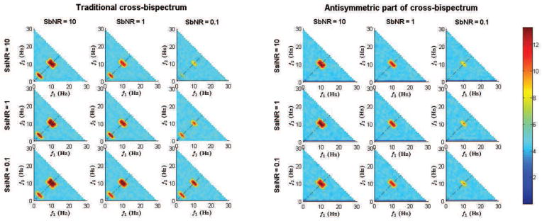
Comparison between the spectral content of the normalized cross-bispectrum and the normalized antisymmetric part of the cross-bispectrum for all combinations of SbNR and SsiNR. Data from one representative case among all simulation repetitions.
We observe that, in all cases, the antisymmetric part of cross-bispectrum suppresses the interaction peak shown by traditional cross-bispectrum at frequency pair (3Hz,3Hz), which was actually generated only by self-interacting sources. Moreover, the magnitude of the antisymmetric part of the cross-bispectrum (whose value is indicated by color) does not depend on SsiNR, contrary to the magnitude of the traditional cross-bispectrum which increases for decreasing SsiNR, that is for increasing nonlinear self-interacting noise. This was taken as first evidence that the our metric is not biased by the activity self-interacting sources. Conversely, both bijk(f1, f2) and b[i|j|k](f1, f2) are affected by background noise level, as their magnitude decrease for decreasing SbNR.
The interaction detected by the two metrics at (10Hz, 10Hz) was then fitted by model equations 17 and 25. The results are summarized in figure 3. In the top panels, the correlation between true and estimated source topographies is shown for the traditional cross-bispectrum (on the left) and for its antisymmetric part (on the right). In particular, we plotted the histograms of 1/(1 − r), with r being the second of of the two canonical correlation coefficients. Here, the correlation is used to quantify the ability of the two metrics in identifying truly interacting sources. We also recall that this value is computed before applying MOCA (and the inverse method therein), while an example of inverse reconstruction of interacting sources, as provided in output by MOCA, is given in the bottom panels of figure 3.
Figure 3.

Top panels: histograms of 1/(1 − r), with r being the second of the two canonical correlation coefficients between true and estimated topographies of interacting sources, for all combinations of SbNR and SsiNR. Bottom panels: an example of recovered brain sources (after MOCA and inverse method therein). The green dots mark the location of truly interacting sources; the green crosses mark the location of self-interacting sources.
We first note that both correlation values and source reconstruction are slightly affected by SbNR, while the main differences in using the traditional cross-bispectrum and its antisymmetric part depend on SsiNR. For SsiNR=10, namely for low level of self-interacting noise, both metrics successfully identify truly interacting sources. For SsiNR=1, namely for medium level of self-interacting noise, the antisymmetric part is still able to recognize truly interacting sources while the performances of the traditional cross-bispectrum become poorer, as revealed by i) lower values of correlation coefficients and ii) the appearance of ghosts in source reconstruction at the locations of self-interacting sources. However, for SsiNR=0.1, namely for high level of self-interacting noise, also the antisymmetric part of the cross-bispectrum is biased by self-interacting sources. This was explained as evidence that, in presence of strong non-linear noise, the symmetric components of bispectra may be not suppressed completely for finite length data.
We finally evaluated the ability of the antisymmetric part of the cross-bispectrum to provide more robust estimates of the phase difference between interacting sources than i) the traditional cross-bispectrum and ii) the cross-spectrum. A comparison between the results obtained by using the three methods are shown in figure 4. Here, data have been plotted in the range [0;1.2] and the vertical dashed lines mark the true simulated value, i.e., Δϕ = 0.628.
Figure 4.

Estimation of phase difference between interacting sources obtained by using: i) the traditional cross-bispectrum (top left), ii) the antisymmetric part of the cross-bispectrum (top right) and iii) cross spectra (bottom), for all combinations of SbNR and SsiNR. The vertical dashed line denotes the true value of phase difference, i.e., Δϕ = 0.628. m and s denote the mean value and the standard deviation, respectively. Data from all simulation repetitions.
We note that, similarly to correlation coefficients, the results of phase estimation are moderately affected by the background noise level. In particular, we observe a slight shift of the main peak of the histograms towards lower values for of high background noise level (SbNR=0.1). Furthermore, the main differences between the three methods rely only on the self-interacting noise level. In particular, for low self-interacting noise level (SsiNR=10), all the three methods provide reliable estimates of the phase difference. For increasing self-interacting noise level (SsiNR=1) the performance of the antisymmetric part of the cross-bispectrum is slightly affected, while we can observe: i) a higher variability of results for the traditional cross-bispectrum, as measured by the standard deviation of the estimates; ii) a drift towards lower values for the main peak in the estimate distribution of the cross-spectra, as was expected since the real parts of cross-spectra are corrupted by self-interacting sources. Finally, for high self interacting noise level (SsiNR=0.1) both the traditional cross-bispectrum and its antisymmetric part do not provide a stable estimation of the phase difference, being this result dependent on the performance of the fit.
3.2. Real EEG recordings
We first analyzed the antisymmetric part of the cross-bispectrum, B[i|j|k](f1, f2), of all subjects in order to identify those who exhibited a significant interaction signal. As outlined in the previous section, we looked at its normalized form, b[i|j|k], (rather than B[i|j|k] itself) since, while still proportional to the strength of the interaction, it suppresses the spurious peaks resulting from high variance of the estimates. We observed significant values of the antisymmetric part of the cross-bispectrum in approximately one-half of all subjects (9 out of 20). For these subjects, hereinafter referred to as Subject 1–9, the antisymmetric part of the cross-bispectrum showed one significant peak at around the frequency pair (f1, f2) = (10Hz, 10Hz), reflecting a cross-frequency interaction between sources of alpha- and beta-band signals, namely at around f1 = f2 = 10 Hz and f3 = f1 + f2 = 20 Hz. However, a certain amount of intersubject variability in channel and source topographies was also observed. The remaining subjects did not show significant interactions and, thus, were dropped out from the analysis. In the following, we will illustrate the results from a few subjects chosen from those exhibiting a significant interaction signal and which best reflect the observed intersubject variability.
From a comparison between the cross-bispectrum and its antisymmetric part, we found interesting differences which are described below. By looking at their frequency profiles, we found that the antisymmetric part of the cross-bispectrum effectively suppressed peaks in the cross-bispectrum, which were thus attributed to self-interaction phenomena. As an example, in figure 5 we show the results from Subjects 1 and 5, distinguished in two panels, for which the differences were more clear. In each panel, both the normalized cross-bispectrum bijk(f1, f2) (on the left) and the normalized antisymmetric part of the cross-bispectrum b[i|j|k](f1, f2) (on the right) are shown. The plots read as follows. In the upper part, the magnitudes of bijk(f1, f2) and b[i|j|k](f1, f2) are shown as function of frequencies f1 and f2 up to f1 + f2 = 50 Hz. Moreover, since the main peaks always occured at frequency pairs located on the diagonal axis f2 = f1, the magnitudes of bijk(f1, f2) and b[i|j|k](f1, f2) for f2 = f1 are shown separately in the bottom part of each plot, where the reader can appreciate the values obtained for each channel triplet. In the top panel, we note that the normalized cross-bispectrum has a broad maximum, peaking at two frequency pairs, i.e., (10Hz,10Hz) and (12Hz,12Hz), which reflects a significant phase synchronization between signal components lying in the alpha and beta bands. However, when looking at the normalized antisymmetric part of the cross-bispectrum, we note that the interaction at (12Hz,12Hz) is less prominent, and thus the larger peak in the normalized cross-bispectrum magnitude was possibly generated by self interactions. Therefore, only the frequency pair at around (10Hz,10Hz) has to be considered for connectivity analysis. Similarly, in the bottom panel, we observe that the normalized antisymmetric part of the cross-bispectrum keeps only the peak at around (11Hz,11Hz), while suppresses the peaks at around (20Hz,20Hz), (22Hz,11Hz) and (11Hz,22Hz), possibly generated by self interaction processes, e.g., higher harmonic generation.
Figure 5.

Comparison between the normalized cross-bispectrum bijk(f1, f2) (on the left) and the normalized antisymmetric part of the cross-bispectrum b[i|j|k](f1, f2) (on the right). Data from Subject 1 (top panel) and Subject 5 (bottom panel).
We further investigated the differences between the cross-bispectrum and its antisymmetric part by analysing their channel topographies. We found that, as opposed to the cross-bispectrum, the spatial pattern of its antisymmetric part was straightforwardly interpretable in terms of underlying source interactions. An example is given in figure 6. Here, the magnitude of the antisymmetric part of the cross-bispectrum, i.e., |B[i|j|k](f̃1, f̃2)|, at frequency pair of maximum interaction, i.e., (f̃1, f̃2) = (10Hz, 10Hz) is shown for Subject 1. We refer to figure 1 for a comparison with the cross-bispectrum magnitude for the same data set. We observe that both the cross-bispectrum (figure 1) and its antisymmetric part (figure 6) reveal an interaction between EEG activities in the occipital, parietal and central regions. However, while in figure 1 we observe an high cross-bispectrum between nearby electrodes, which is consistent with uniform distributed independent sources, the antisymmetric part of the cross-bispectrum (figure 6) reflects an interesting interaction structure: the parietal electrodes are mostly interacting with the occipital and the central ones, and vice versa. This structure is more evident in the maps of figure 7, where we display the antisymmetric part of the cross-bispectrum (here, the real and the imaginary components are shown separately) for a small subset of actual recording channels, i.e., at the approximate locations of 20 electrodes of the international 10–20 system. In particular, we wish to point out that, within each small circle, the bispectral map still has the spatial resolution of the 98 channel system. Moreover, we marked the locations of all the 20 electrodes and highlighted with a circled black dot the electrode with respect to which the cross-bispectrum is calculated.
Figure 6.

Magnitude of the antisymmetric part of the cross-bispectrum between all channel pairs, B[i|i|k], at frequency pair (10Hz, 10Hz). Data from Subject 1.
Figure 7.
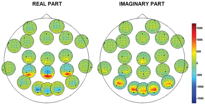
Real and imaginary components of the antisymmetric part of the cross-bispectrum, B[i|i|k], at frequency pair (10Hz, 10Hz) for a subset of actual recording channels. Data from Subject 1.
In summary, as opposed to the cross-bispectrum, the spatial pattern of its antisymmetric part was able to reveal an interaction between distinct sources, located in the parietal and occipital/central regions.
We finally carried out the localization of interacting sources by using the strategy described in the method section. As pointed out at the beginning of this section, a certain amount of individual variability was observed both at channel and at source level. Then, to summarize the obtained results, in figure 8 we show the localized electrical activities (top row) and the corresponding scalp potentials (bottom row) for 5 subjects which best reflect the observed variability. In particular, Subject 1 showed an interacting system composed by one source located in the occipital and central regions (source A) and one source located in the parietal region (source B), thus confirming what was expected from the analysis of the bispectral maps in figures 6 and 7. A similar correspondence between brain source localization and bispectral maps was observed in all the other subjects.
Figure 8.

Localization of interacting source activities (top row) and the corresponding scalp potentials (bottom row). The plot uses arbitrary color units. Data from Subjects 1–5.
4. Discussion
In this paper, we propose to use the antisymmetric part of third order statistical moments, i.e. cross-bispectra, as a nonlinear measure of functional connectivity. The reason comes from the observation that these components cannot be generated from mixtures of independent sources but solely reflect the existence of genuine interactions.
The proposed method allows to detect functional quadratic phase coupling between brain sources and to localize their generators. A key step to identify such quadratic phase couplings from cross-bispectra is that of being able to reject spurious, i.e. non-significant, occurrences which are often found in real data analysis. Indeed, the absence of a quadratic phase coupling would produce no peaks in cross-bispectrum only for data of an infinite length. However, due to the finite length encountered in practice, spurious peaks may appear in the cross-bispectrum and in its antisymmetric part. To assess statistical significance of the peaks, we here adopted a normalization procedure in which the cross-bispectral values are divided by the standard deviation of their estimates. Specifically, the real and the imaginary part of complex cross-bispectral values are normalized separately. We observed in simulations that a reasonable threshold value for the magnitude of the normalized antisymmetric part of the cross-bispectrum to be distinguishable from values generated by pure Gaussian noise for finite data length (e.g., 600 s) was found to be about 5. Other possible normalization could be used to the same end: e.g., the use of a pooled estimator for the standard deviations of the real and the imaginary part of cross-bispectra.
The above identified interactions were fitted to a two source model, and their topographies were localized using a linear inverse method and demixed using MOCA. This was based on the assumption that i) all observed interactions are pairwise; ii) the linear solver is adequate; and iii) the sources have a minimum overlap (MOCA constraint). The last assumption is necessary because the topographies of the two sources for each pair are only unique up to a mixing factor, mathematically similar to the case of an eigenvector decomposition of a matrix with eigenvalues coming in pairs. To generalize our approach, all these three assumptions could be replaced by others. First, we could extend the interaction model to allow for more than two interacting sources. In this case, the model equation to be fitted to data would include more additive terms similar to those at the right-hand side of equation 17, representing all possible relationships between brain sources taken in pairs or triplets. Also in this case the non-uniqueness of the solution needs to be faced. To this purpose, a generalization of the MOCA-algorithm able to take into account systems composed by more than two sources is presented in Nolte et al. (2009). However, fitting this more complicated model to the data might be less straightforward. We did not investigate this possibility in the present work, but multilinear decomposition methods (see, e.g., Kolda and Bader, 2009) are a possible approach to face this issue. Second, for the inverse method, an alternative is to use RAP-MUSIC similarly to what done by (Shahbazi Avarvand et al., 2012) to analyze the singular vectors of the imaginary part of the cross-spectra. In contrast to the present approach, RAP-MUSIC assumes dipolar sources, which, trivially, is an advantage if the assumption is true, because the variance is reduced, and a disadvantage if not, because the bias is increased. In any event, also RAP-MUSIC would fail in general if three sources are interacting with each other but spanning only a two-dimensional subspace of the sensor space. This situation is analogous to applying RAP-MUSIC to covariance matrices for perfectly correlated sources which would also lead to a collapse of signal dimension in sensor space. With the present techniques such cases cannot be treated. We will address these problems in a future work.
The proposed method was first tested in simulations. The simulations showed that the antisymmetric part of the cross-bispectrum allows to identify interacting sources in most circumstances where the traditional cross-bispectrum is confounded by non-linear noisy sources. We also observed that, if noisy sources are very strong, our metric is still able to detect the presence of an interaction, but further analysis, such as fitting an interaction model to the data, is possibly affected by the noise bias. This is essentially due to the fact that, in the computation of the antisymmetric part of cross-bispectra, the contribution of non-linear non-interacting sources is suppressed in a statistical sense and, if too large, it may be not completely removed. Simulations allowed us also to compare phase estimations obtained with the antisymmetric part of the cross-bispectrum to phase estimation from linear metrics that we previously introduced to study linear interactions robust to mixing artifacts. This was achieved by simulating a particular interaction, namely the delayed coupling between two non-linear sources, which implies the synchronization between rhythms both at the same and at different frequencies and, thus, both linear and nonlinear measures can be used complementarily to analyze interaction dynamics. The antisymmetric part of the cross-bispectrum offers an advantage over the aforementioned linear approaches since it results in complex-valued quantities which contain phase information related to source interaction. On the other hand, the physical interpretation of the phase of the antisymmetric part of the cross-bispectrum might be complicated, depending on the nature of the interaction. In this work, we gave explicit interpretations in the following two cases: i) a pure nonlinear interaction between two sources whose activities are contributed by oscillations at different frequencies; ii) interaction between two sources with intrinsic nonlinear dynamic and which are time-delayed copies. The latter case was explored in our simulations showing that the antisymmetric part of the cross-bispectrum exhibits better performances then cross-spectrum in recovering the phase difference between interacting sources.
The analysis pipeline was applied to real EEG data recorded during eyes-open resting state. The approach revealed an interaction occurring between brain sources at 10 Hz and 20 Hz in about half of the measured subjects. A possible reason for this is given by a general practical problem of nonlinear methods: nonlinear phenomena are typically weaker than linear ones. Indeed, the observed interactions were mainly occurring between 10 Hz and 20 Hz, which are the most pronounced rhythms at rest. Even though couplings between other frequencies are possibly observable, the spectral content is surely richer when using linear methods. Moreover, the observed topographies for interacting sources are less stable than those usually obtained from second order moments. In our data interacting sources are localized, for all subjects showing meaningful results for the antisymmetric part of cross-bispectra, in occipito-parietal and central areas, consistently with previous observations (Palva et al., 2005). Indeed, when dealing with non linear approaches, we are faced with a trade-off: if a nonlinear signal can be observed, a deeper insight into brain dynamic is possible but such signals are more difficult to detect consistently in all subjects. Nevertheless, non linear dynamics might represent a key mechanism for brain interaction: cross-frequency phase synchronization have been recognized to be a mechanism for different networks to interact and integrate spectrally distributed processing (Palva et al., 2005). In this framework, cross-frequency phase synchronization between alpha and beta rhythms is already known to occur at rest (Nikulin and Brismar, 2006; Nikulin et al., 2011) and to be modulated by task and shown to be involved in the coordination between attention and perception (Palva et al., 2005).
Although, a comprehensive comparison with other non linear methods is beyond the scope of this work, we want to emphasize that our method is based on third order moments which are a “pure” nonlinearity in the sense that for Gaussian distributed data these moments vanish apart from random fluctuations. This is a substantial difference to many other nonlinear measures, e.g., the phase locking value (Lachaux et al., 1999) which does not vanish for Gaussian distributions and which measures properties of phase distributions well consistent with Gaussian distributions (Aydore et al., 2013). It is hence unclear whether an interaction observed with phase locking cannot equally be observed with coherence. Similarly, transfer entropy (Schreiber, 2000), which is a nonlinear measure of effective connectivity, is formally equivalent to Granger Causality for Gaussian distributed data. Also, correlations of power of signals at the same frequency can always be expressed as functions of complex coherency which follows from the fact that cross-spectra form a complete and sufficient statistics for Gaussian distributed and zero-mean stationary processes. Methods based on correlations of power designed to remove artifacts of volume conduction were suggested in Brookes et al. (2012) and in Hipp et al. (2012). These methods are based on the orthogonalization of segments of data between pairs of sensors in the time-domain and in the frequency domain, respectively. It is an open question, under which conditions this orthogonalization actually removes rather than just attenuates artifacts of volume conduction.
Functional connectivity based on the antisymmetric part of cross-bispectra for EEG and MEG can also be estimated directly between brain source activities. An appealing framework would be the characterization of resting state network (RSNs) (Deco and Corbetta, 2011) phenomenon. Frequency specific coupling in RSNs have been recently studied with the imaginary part of coherency (Marzetti et al., 2013; Martino et al., 2011) as well as with correlation of power (Betti et al., 2013; Brookes et al., 2011; de Pasquale et al., 2010; de Pasquale et al., 2012; Hipp et al., 2012). All these approaches have investigated coupling between brain regions at the same frequency, with an emphasis on phase coupling or on amplitude coupling. Conversely, the proposed method, while being intrinsically robust to mixing artifacts, is designed to reveal cross-frequency interactions or might serve as a basis for getting further insight into the study of phase delayed coupling at a given frequency.
In conclusion, we believe that the proposed method might provide a new framework for further understanding the role of brain rhythms in the functional integration and segregation of brain networks.
Highlights.
We investigate cross-frequency coupling in EEG using third order spectral analysis.
We generalize the properties of imaginary part of cross-spectrum to nonlinear case.
The antisymmetrized cross-bispectra offer reduced sensitivity to mixture artifacts.
We demonstrate non linear coupling between cortical loci at specific frequency pairs.
Acknowledgments
This work was partially supported by the “Mapping the Human Connectome Structure, Function, and Heritability” (1U54MH091657-01) from the 16 National Institutes of Health Institutes and Centers that support the NIH Blueprint for Neuroscience Research, by the Italian Ministry of Education, University and Research (PRIN 2010–2011 n. 2010SH7H3F 006 “Functional connectivity and neuroplasticity in physiological and pathological aging”) and by grants from the EU (ERC-2010-AdG-269716), the DFG (SFB 936/A3), and the BMBF (031A130).
Appendix A
Let us consider the antisymmetric part of the cross-bispectrum between three channel recordings, namely i, j and k, as defined in equation 17:
| (A.1) |
where α(f1, f2) and β(f1, f2) are complex valued functions and ai and bi, i = i, j, k, are the real valued topographies of the two interacting sources at those channels. Let us now replace ai and bi, i = i, j, k, by a linear mixture of them, i.e.,
| (A.2) |
with arbitrary coefficients A, B, C and D. For simplicity, we will use the matrix notation by collecting the coefficients in a 2×2 mixing matrix Γ, i.e.,
| (A.3) |
In general, the above substitution also changes the antisymmetric part of the cross-bispectrum, which depends on source topographies. Therefore, if we want to keep unchanged the value of B[i|j|k], we also have to replace α(f1, f2) and β(f1, f2) by new complex functions α′(f1, f2) and β′(f1, f2), i.e.,
| (A.4) |
In particular, by combining the equations A.2 and A.4, we get:
| (A.5) |
Then, a straightforward comparison of equations A.5 and A.1 yields to:
| (A.6) |
or, in matrix notation,
| (A.7) |
where ΓT is the transpose of the mixing matrix.
Hence, according to equation A.7, the antisymmetric part of the cross-bispectrum is invariant to the arbitrary linear combination of source topographies defined in equation A.2, if we simultaneously take α′(f1, f2) and β′(f1, f2) such that:
| (A.8) |
Footnotes
It is common to denote the antisymmetrizing operation on tensor indices by a bracket notation in which [·] indicates antisymmetrization over subset of indices included in the brackets, e.g., Bi[jk] = Bijk − Bikj. In the event that indices to be antisymmetrized are not adjacent to each other, the preceding notation is extended by using vertical lines to exclude indices from the antisymmetrization, i.e.: B[i|j|k] = Bijk − Bkji.
6. Conflict of interest
The authors disclose any actual or potential conflict of interest.
Publisher's Disclaimer: This is a PDF file of an unedited manuscript that has been accepted for publication. As a service to our customers we are providing this early version of the manuscript. The manuscript will undergo copyediting, typesetting, and review of the resulting proof before it is published in its final citable form. Please note that during the production process errors may be discovered which could affect the content, and all legal disclaimers that apply to the journal pertain.
References
- Aydore S, Pantazis D, Leahy RM. A note on the phase locking value and its properties. NeuroImage. 2013;74 (0):231–244. doi: 10.1016/j.neuroimage.2013.02.008. URL http://www.sciencedirect.com/science/article/pii/S1053811913001286. [DOI] [PMC free article] [PubMed] [Google Scholar]
- Barnett TP, Johnson LC, Naitoh P, Hicks N, Nute C. Bispectrum analysis of electroencephalogram signals during waking and sleeping. Science. 1971;172 (3981):401–402. doi: 10.1126/science.172.3981.401. URL http://www.sciencemag.org/content/172/3981/401.abstract. [DOI] [PubMed] [Google Scholar]
- Betti V, Penna SD, de Pasquale F, Mantini D, Marzetti L, Romani GL, Corbetta M. Natural scenes viewing alters the dynamics of functional connectivity in the human brain. Neuron. 2013;79 (4):782–797. doi: 10.1016/j.neuron.2013.06.022. URL http://www.sciencedirect.com/science/article/pii/S0896627313005382. [DOI] [PMC free article] [PubMed] [Google Scholar]
- Brookes MJ, Hale JR, Zumer JM, Stevenson CM, Francis ST, Barnes GR, Owen JP, Morris PG, Nagarajan SS. Measuring functional connectivity using MEG: Methodology and comparison with fcmri. NeuroImage. 2011;56 (3):1082–1104. doi: 10.1016/j.neuroimage.2011.02.054. URL http://www.sciencedirect.com/science/article/pii/S1053811911002102. [DOI] [PMC free article] [PubMed] [Google Scholar]
- Brookes MJ, Woolrich MW, Barnes GR. Measuring functional connectivity in MEG: A multivariate approach insensitive to linear source leakage. NeuroImage. 2012;63 (2):910–920. doi: 10.1016/j.neuroimage.2012.03.048. URL http://www.sciencedirect.com/science/article/pii/S1053811912003291. [DOI] [PMC free article] [PubMed] [Google Scholar]
- Bullock TH, Achimowicz JZ, Duckrow RB, Spencer SS, Iragui-Madoz VJ. Bicoherence of intracranial EEG in sleep, wakefulness and seizures. Electroencephalography and Clinical Neurophysiology. 1997;103 (6):661–678. doi: 10.1016/s0013-4694(97)00087-4. URL http://www.sciencedirect.com/science/article/pii/S0013469497000874. [DOI] [PubMed] [Google Scholar]
- Darvas F, Miller KJ, Rao RPN, Ojemann JG. Nonlinear phase-phase cross-frequency coupling mediates communication between distant sites in human neocortex. The Journal of Neuroscience. 2009a;29 (2):426–435. doi: 10.1523/JNEUROSCI.3688-08.2009. URL http://www.jneurosci.org/content/29/2/426.abstract. [DOI] [PMC free article] [PubMed] [Google Scholar]
- Darvas F, Ojemann JG, Sorensen LB. Bi-phase locking - a tool for probing non-linear interaction in the human brain. NeuroImage. 2009b;46 (1):123–132. doi: 10.1016/j.neuroimage.2009.01.034. URL http://www.sciencedirect.com/science/article/pii/S1053811909000949. [DOI] [PMC free article] [PubMed] [Google Scholar]
- de Pasquale F, Della Penna S, Snyder AZ, Lewis C, Mantini D, Marzetti L, Belardinelli P, Ciancetta L, Pizzella V, Romani GL, Corbetta M. Temporal dynamics of spontaneous MEG activity in brain networks. Proceedings of the National Academy of Sciences. 2010;107 (13):6040–6045. doi: 10.1073/pnas.0913863107. URL http://www.pnas.org/content/107/13/6040.abstract. [DOI] [PMC free article] [PubMed] [Google Scholar]
- de Pasquale F, Della Penna S, Snyder AZ, Marzetti L, Pizzella V, Romani GL, Corbetta M. A cortical core for dynamic integration of functional networks in the resting human brain. Neuron. 2012;74 (4):753–764. doi: 10.1016/j.neuron.2012.03.031. URL http://www.sciencedirect.com/science/article/pii/S089662731200342X. [DOI] [PMC free article] [PubMed] [Google Scholar]
- Deco G, Corbetta M. The dynamical balance of the brain at rest. The Neuroscientist. 2011;17 (1):107–123. doi: 10.1177/1073858409354384. URL http://nro.sagepub.com/content/17/1/107.abstract. [DOI] [PMC free article] [PubMed] [Google Scholar]
- Dumermuth G, Huber PJ, Kleiner B, Gasser T. Analysis of the interrelations between frequency bands of the EEG by means of the bispectrum a preliminary study. Electroencephalography and Clinical Neurophysiology. 1971;31 (2):137–148. doi: 10.1016/0013-4694(71)90183-0. URL http://www.sciencedirect.com/science/article/pii/0013469471901830. [DOI] [PubMed] [Google Scholar]
- Fonov V, Evans AC, Botteron K, Almli CR, McKinstry RC, Collins DL. Unbiased average age-appropriate atlases for pediatric studies. NeuroImage. 2011;54 (1):313–327. doi: 10.1016/j.neuroimage.2010.07.033. URL http://www.sciencedirect.com/science/article/pii/S1053811910010062. [DOI] [PMC free article] [PubMed] [Google Scholar]
- Fonov VS, Evans AC, McKinstry RC, Almli CR, Collins DL. Unbiased nonlinear average age-appropriate brain templates from birth to adulthood. NeuroImage. 2009;47(Supplement 1 )(0):S102. URL http://www.sciencedirect.com/science/article/pii/S1053811909708845. [Google Scholar]
- Fries P. Neuronal gamma-band synchronization as a fundamental process in cortical computation. Annual Review of Neuroscience. 2009;32 (1):209–224. doi: 10.1146/annurev.neuro.051508.135603. URL http://www.annualreviews.org/doi/abs/10.1146/annurev.neuro.051508.135603. [DOI] [PubMed] [Google Scholar]
- Gómez-Herrero G, Atienza M, Egiazarian K, Cantero JL. Measuring directional coupling between EEG sources. NeuroImage. 2008;43 (3):497–508. doi: 10.1016/j.neuroimage.2008.07.032. URL http://www.sciencedirect.com/science/article/pii/S1053811908008549. [DOI] [PubMed] [Google Scholar]
- Gross J, Schmitz F, Schnitzler I, Kessler K, Shapiro K, Hommel B, Schnitzler A. Anticipatory control of long-range phase synchronization. European Journal of Neuroscience. 2006;24 (7):2057–2060. doi: 10.1111/j.1460-9568.2006.05082.x. URL http://dx.doi.org/10.1111/j.1460-9568.2006.05082.x. [DOI] [PubMed] [Google Scholar]
- Helbig M, Schwab K, Leistritz L, Eiselt M, Witte H. Analysis of time-variant quadratic phase couplings in the tracé alternant EEG by recursive estimation of 3rd-order time-frequency distributions. Journal of Neuroscience Methods. 2006;157 (1):168–177. doi: 10.1016/j.jneumeth.2006.04.012. URL http://www.sciencedirect.com/science/article/pii/S0165027006001890. [DOI] [PubMed] [Google Scholar]
- Hipp JF, Hawellek DJ, Corbetta M, Siegel M, Engel AK. Large-scale cortical correlation structure of spontaneous oscillatory activity. Nat Neurosci. 2012;15:884–890. doi: 10.1038/nn.3101. URL http://dx.doi.org/10.1038/nn.3101. [DOI] [PMC free article] [PubMed] [Google Scholar]
- Hyvärinen A, Zhang K, Shimizu S, Hoyer PO. Estimation of a structural vector autoregression model using non-gaussianity. Journal of Machine Learning Research. 2010 Aug;11:1709–1731. URL http://dl.acm.org/citation.cfm?id=1756006.1859907. [Google Scholar]
- Jirsa V, Müller V. Cross-frequency coupling in real and virtual brain networks. Frontiers in Computational Neuroscience. 2013;7(78) doi: 10.3389/fncom.2013.00078. URL http://www.frontiersin.org/computationalneuroscience/10.3389/fncom.2013.00078/abstract. [DOI] [PMC free article] [PubMed] [Google Scholar]
- Johansen JW, Sebel PS. Development and clinical application of electroencephalographic bispectrum monitoring. Anesthesiology. 2000;93:1336–1344. doi: 10.1097/00000542-200011000-00029. URL http://journals.lww.com/anesthesiology/Fulltext/2000/11000/Development_and_Clinical_Application_of.29.aspx. [DOI] [PubMed] [Google Scholar]
- Kolda T, Bader B. Tensor decompositions and applications. SIAM Review. 2009;51 (3):455–500. URL http://epubs.siam.org/doi/abs/10.1137/07070111X. [Google Scholar]
- Lachaux JP, Rodriguez E, Martinerie J, Varela FJ. Measuring phase synchrony in brain signals. Human Brain Mapping. 1999;8 (4):194–208. doi: 10.1002/(SICI)1097-0193(1999)8:4<194::AID-HBM4>3.0.CO;2-C. URL http://dx.doi.org/10.1002/(SICI)1097-0193(1999)8:4<194::AID-HBM4>3.0.CO;2-C. [DOI] [PMC free article] [PubMed] [Google Scholar]
- Martino J, Honma SM, Findlay AM, Guggisberg AG, Owen JP, Kirsch HE, Berger MS, Nagarajan SS. Resting functional connectivity in patients with brain tumors in eloquent areas. Annals of Neurology. 2011;69 (3):521–532. doi: 10.1002/ana.22167. URL http://dx.doi.org/10.1002/ana.22167. [DOI] [PMC free article] [PubMed] [Google Scholar]
- Marzetti L, Del Gratta C, Nolte G. Understanding brain connectivity from EEG data by identifying systems composed of interacting sources. NeuroImage. 2008;42 (1):87–98. doi: 10.1016/j.neuroimage.2008.04.250. URL http://www.sciencedirect.com/science/article/pii/S1053811908005971. [DOI] [PubMed] [Google Scholar]
- Marzetti L, Della Penna S, Snyder A, Pizzella V, Nolte G, de Pasquale F, Romani GL, Corbetta M. Frequency specific interactions of MEG resting state activity within and across brain networks as revealed by the multivariate interaction measure. NeuroImage. 2013;79 (0):172–183. doi: 10.1016/j.neuroimage.2013.04.062. URL http://www.sciencedirect.com/science/article/pii/S1053811913004096. [DOI] [PMC free article] [PubMed] [Google Scholar]
- Marzetti L, Nolte G, Perrucci MG, Romani GL, Del Gratta C. The use of standardized infinity reference in EEG coherency studies. NeuroImage. 2007;36 (1):48–63. doi: 10.1016/j.neuroimage.2007.02.034. URL http://www.sciencedirect.com/science/article/pii/S105381190700122X. [DOI] [PubMed] [Google Scholar]
- Miller KJ, Weaver KE, Ojemann JG. Direct electrophysiological measurement of human default network areas. Proceedings of the National Academy of Sciences. 2009;106 (29):12174–12177. doi: 10.1073/pnas.0902071106. URL http://www.pnas.org/content/106/29/12174.abstract. [DOI] [PMC free article] [PubMed] [Google Scholar]
- Nikias CL, Petropulu AP. Prentice Hall signal processing series. PTR Prentice Hall; 1993. Higher-order spectra analysis: a nonlinear signal processing framework. URL http://books.google.it/books?id=DhSAAAAMAAJ. [Google Scholar]
- Nikulin VV, Brismar T. Phase synchronization between alpha and beta oscillations in the human electroencephalogram. Neuroscience. 2006;137 (2):647–657. doi: 10.1016/j.neuroscience.2005.10.031. URL http://www.sciencedirect.com/science/article/pii/S0306452205011711. [DOI] [PubMed] [Google Scholar]
- Nikulin VV, Nolte G, Curio G. A novel method for reliable and fast extraction of neuronal EEG/MEG oscillations on the basis of spatio-spectral decomposition. NeuroImage. 2011;55 (4):1528–1535. doi: 10.1016/j.neuroimage.2011.01.057. URL http://www.sciencedirect.com/science/article/pii/S1053811911000930. [DOI] [PubMed] [Google Scholar]
- Nocedal J, Wright S. Springer Series in Operations Research and Financial Engineering. Springer; 2006. Numerical Optimization. URL http://books.google.it/books?id=eNlPAAAAMAAJ. [Google Scholar]
- Nolte G, Bai O, Wheaton L, Mari Z, Vorbach S, Hallett M. Identifying true brain interaction from EEG data using the imaginary part of coherency. Clinical Neurophysiology. 2004;115 (10):2292–2307. doi: 10.1016/j.clinph.2004.04.029. URL http://www.sciencedirect.com/science/article/pii/S1388245704001993. [DOI] [PubMed] [Google Scholar]
- Nolte G, Marzetti L, Valdes Sosa P. Minimum overlap component analysis (MOCA) of EEG/MEG data for more than two sources. Journal of Neuroscience Methods. 2009;183 (1):72–76. doi: 10.1016/j.jneumeth.2009.07.006. URL http://www.sciencedirect.com/science/article/pii/S0165027009003690. [DOI] [PubMed] [Google Scholar]
- Nolte G, Ziehe A, Nikulin VV, Schlögl A, Krämer N, Brismar T, Müller K-R. Robustly estimating the flow direction of information in complex physical systems. Phys Rev Lett. 2008 Jun;100:234101. doi: 10.1103/PhysRevLett.100.234101. URL http://link.aps.org/doi/10.1103/PhysRevLett.100.234101. [DOI] [PubMed] [Google Scholar]
- Nunez PL, Srinivasan R, Westdorp AF, Wijesinghe RS, Tucker DM, Silberstein RB, Cadusch PJ. EEG coherency: I: statistics, reference electrode, volume conduction, laplacians, cortical imaging, and interpretation at multiple scales. Electroencephalography and Clinical Neurophysiology. 1997;103 (5):499–515. doi: 10.1016/s0013-4694(97)00066-7. URL http://www.sciencedirect.com/science/article/pii/S0013469497000667. [DOI] [PubMed] [Google Scholar]
- Palva JM, Palva S, Kaila K. Phase synchrony among neuronal oscillations in the human cortex. The Journal of Neuroscience. 2005;25 (15):3962–3972. doi: 10.1523/JNEUROSCI.4250-04.2005. URL http://www.jneurosci.org/content/25/15/3962.abstract. [DOI] [PMC free article] [PubMed] [Google Scholar]
- Pascual-Marqui RD. Discrete, 3D distributed, linear imaging methods of electric neuronal activity. Part 1: exact, zero error localization. ArXiv e-prints 2007a Oct; [Google Scholar]
- Pascual-Marqui RD. Instantaneous and lagged measurements of linear and nonlinear dependence between groups of multivariate time series: frequency decomposition. ArXiv e-prints 2007b Nov; [Google Scholar]
- Pascual-Marqui RD. Quantitative EEG Analysis: Methods and Clinical Applications. In: Tong S, Thakor NV, editors. Ch Theory of the EEG Inverse Problem. Chapter 5. Artech House; Boston: 2009. pp. 121–140. [Google Scholar]
- Pascual-Marqui RD, Lehmann D, Koukkou M, Kochi K, Anderer P, Saletu B, Tanaka H, Hirata K, John ER, Prichep L, Biscay-Lirio R, Kinoshita T. Assessing interactions in the brain with exact low-resolution electromagnetic tomography. Philosophical Transactions of the Royal Society A: Mathematical, Physical and Engineering Sciences. 2011;369 (1952):3768–3784. doi: 10.1098/rsta.2011.0081. URL http://rsta.royalsocietypublishing.org/content/369/1952/3768.abstract. [DOI] [PubMed] [Google Scholar]
- Pereda E, Quiroga RQ, Bhattacharya J. Nonlinear multivariate analysis of neurophysiological signals. Progress in Neurobiology. 2005;77 (1–2):1–37. doi: 10.1016/j.pneurobio.2005.10.003. URL http://www.sciencedirect.com/science/article/pii/S030100820500119X. [DOI] [PubMed] [Google Scholar]
- Schoffelen JM, Gross J. Source connectivity analysis with MEG and EEG. Human Brain Mapping. 2009;30 (6):1857–1865. doi: 10.1002/hbm.20745. URL http://dx.doi.org/10.1002/hbm.20745. [DOI] [PMC free article] [PubMed] [Google Scholar]
- Schreiber T. Measuring information transfer. Phys Rev Lett. 2000 Jul;85:461–464. doi: 10.1103/PhysRevLett.85.461. URL http://link.aps.org/doi/10.1103/PhysRevLett.85.461. [DOI] [PubMed] [Google Scholar]
- Schwilden H. Concepts of EEG processing: from power spectrum to bispectrum, fractals, entropies and all that. Best Practice and Research Clinical Anaesthesiology. 2006;20 (1):31–48. doi: 10.1016/j.bpa.2005.09.001. URL http://www.sciencedirect.com/science/article/pii/S1521689605000728. [DOI] [PubMed] [Google Scholar]
- Sekihara K, Owen J, Trisno S, Nagarajan S. Removal of spurious coherence in MEG source-space coherence analysis. Biomedical Engineering, IEEE Transactions on. 2011;58 (11):3121–3129. doi: 10.1109/TBME.2011.2162514. [DOI] [PMC free article] [PubMed] [Google Scholar]
- Shahbazi Avarvand F, Ewald A, Nolte G. Localizing true brain interactions from EEG and MEG data with subspace methods and modified beamformers. Computational and Mathematical Methods in Medicine. 2012;2012 doi: 10.1155/2012/402341. URL http://dx.doi.org/10.1155/2012/402341. [DOI] [PMC free article] [PubMed] [Google Scholar]
- Shils JL, Litt M, Skolnick BE, Stecker MM. Bispectral analysis of visual interactions in humans. Electroencephalography and Clinical Neurophysiology. 1996;98 (2):113–125. doi: 10.1016/0013-4694(95)00230-8. URL http://www.sciencedirect.com/science/article/pii/0013469495002308. [DOI] [PubMed] [Google Scholar]
- Srinivasan R, Winter WR, Ding J, Nunez PL. EEG and MEG coherence: Measures of functional connectivity at distinct spatial scales of neocortical dynamics. Journal of Neuroscience Methods. 2007;166 (1):41–52. doi: 10.1016/j.jneumeth.2007.06.026. URL http://www.sciencedirect.com/science/article/pii/S016502700700307X. [DOI] [PMC free article] [PubMed] [Google Scholar]
- Stinstra JG, Peters MJ. The volume conductor may act as a temporal filter on the ECG and EEG. Medical and Biological Engineering and Computing. 1998;36 (6):711–716. doi: 10.1007/BF02518873. URL http://dx.doi.org/10.1007/BF02518873. [DOI] [PubMed] [Google Scholar]
- Tallon-Baudry C, Bertrand O, Delpuech C, Pernier J. Stimulus specificity of phase-locked and non-phase-locked 40 hz visual responses in human. The Journal of Neuroscience. 1996;16 (13):4240–4249. doi: 10.1523/JNEUROSCI.16-13-04240.1996. URL http://www.jneurosci.org/content/16/13/4240.abstract. [DOI] [PMC free article] [PubMed] [Google Scholar]
- Van Ness JW. Asymptotic normality of bispectral estimates. The Annals of Mathematical Statistics. 1966;37(5):1257–1272. URL http://www.jstor.org/stable/2239079. [Google Scholar]
- Villa AEP, Tetko IV. Cross-frequency coupling in mesiotemporal EEG recordings of epileptic patients. Journal of Physiology-Paris. 2010;104 (3–4):197–202. doi: 10.1016/j.jphysparis.2009.11.024. URL http://www.sciencedirect.com/science/article/pii/S0928425709001065. [DOI] [PubMed] [Google Scholar]
- Vinck M, Oostenveld R, van Wingerden M, Battaglia F, Pennartz CMA. An improved index of phase-synchronization for electrophysiological data in the presence of volume-conduction, noise and sample-size bias. NeuroImage. 2011;55 (4):1548–1565. doi: 10.1016/j.neuroimage.2011.01.055. URL http://www.sciencedirect.com/science/article/pii/S1053811911000917. [DOI] [PubMed] [Google Scholar]
- Wang X, Chen Y, Ding M. Testing for statistical significance in bispectra: A surrogate data approach and application to neuroscience. Biomedical Engineering, IEEE Transactions on. 2007;54 (11):1974–1982. doi: 10.1109/TBME.2007.895751. [DOI] [PubMed] [Google Scholar]
- Winter WR, Nunez PL, Ding J, Srinivasan R. Comparison of the effect of volume conduction on EEG coherence with the effect of field spread on MEG coherence. Statistics in Medicine. 2007;26 (21):3946–3957. doi: 10.1002/sim.2978. URL http://dx.doi.org/10.1002/sim.2978. [DOI] [PubMed] [Google Scholar]
- Womelsdorf T, Fries P. Neuronal coherence during selective attentional processing and sensory-motor integration. Journal of Physiology-Paris. 2006;100 (4):182–193. doi: 10.1016/j.jphysparis.2007.01.005. URL http://www.sciencedirect.com/science/article/pii/S092842570700006X. [DOI] [PubMed] [Google Scholar]
- Yao D. A method to standardize a reference of scalp EEG recordings to a point at infinity. Physiological Measurement. 2001;22 (4):693. doi: 10.1088/0967-3334/22/4/305. URL http://stacks.iop.org/0967-3334/22/i=4/a=305. [DOI] [PubMed] [Google Scholar]
- Yao D, Wang L, Oostenveld R, Nielsen KD, Arendt-Nielsen L, Chen ACN. A comparative study of different references for EEG spectral mapping: the issue of the neutral reference and the use of the infinity reference. Physiological Measurement. 2005;26 (3):173. doi: 10.1088/0967-3334/26/3/003. URL http://stacks.iop.org/0967-3334/26/i=3/a=003. [DOI] [PubMed] [Google Scholar]