

Abstract
We used microsecond time scale molecular dynamics simulations to compute, at high precision, binding enthalpies for cucurbit[7]uril (CB7) with eight guests in aqueous solution. The results correlate well with experimental data from previously published isothermal titration calorimetry studies, and decomposition of the computed binding enthalpies by interaction type provides plausible mechanistic insights. Thus, dispersion interactions appear to play a key role in stabilizing these complexes, due at least in part to the fact that their packing density is greater than that of water. On the other hand, strongly favorable Coulombic interactions between the host and guests are compensated by unfavorable solvent contributions, leaving relatively modest electrostatic contributions to the binding enthalpies. The better steric fit of the aliphatic guests into the circular host appears to explain why their binding enthalpies tend to be more favorable than those of the more planar aromatic guests. The present calculations also bear on the validity of the simulation force field. Somewhat unexpectedly, the TIP3P water yields better agreement with experiment than the TIP4P-Ew water model, although the latter is known to replicate the properties of pure water more accurately. More broadly, the present results demonstrate the potential for computational calorimetry to provide atomistic explanations for thermodynamic observations.
Introduction
Calorimetric studies of molecular recognition provide not only the free energy of binding but also the breakdown of the free energy into its entropic and enthalpic components.1 Such breakdowns promise insight into the molecular driving forces for binding2−4 and hence guidance in the design of supramolecular systems and of high-affinity ligands for targeted proteins.5−7 However, in practice, calorimetric data often generate new questions and paradoxes. For example, there is still no generally accepted explanation for the widespread phenomenon of entropy–enthalpy compensation,8−13 and although cyclization of small molecule ligands may be expected to reduce the entropy cost of binding, this is by no means consistently observed.14−16 Host–guest systems, which have significantly fewer degrees of freedom than protein–ligand systems, yet still exemplify many of the aforementioned paradoxes,17 are informative and tractable models of molecular recognition with readily available isothermal titration calorimetry (ITC) data.18−21 However, ITC data, regardless of system size, still lack a detailed decomposition of the physical interactions responsible for the measured thermodynamic quantities and therefore cannot yield full explanations of the binding thermodynamics.
Here, we propose the use of atomistic molecular simulations on small host guests systems as a first step toward providing detailed insight into the molecular determinants of binding thermodynamics and thus complementing experimental calorimetry. Previously, calculating well-converged binding enthalpies22−24 has proved challenging,25−ref30 and the low precision of the results has inhibited rigorous comparisons between calculation and experiment. In addition, most computational methods for calculating binding enthalpies, such as by calculating the entropy from the temperature derivative of the binding free energy and subtracting it from the free energy to obtain the enthalpy,25,27,29,30 do not directly provide the decompositions of the binding enthalpy into molecular (e.g., solvent–solvent, solvent–solute, or solute–solute) or force-field component contributions that could provide insight into the molecular basis for the changes in enthalpy associated with molecular recognition.
The present study takes advantage of the dramatic speedup31,32 of molecular simulations afforded by graphical processor units (GPUs) to compute the binding enthalpies of the host cucurbit[7]uril (CB7) with five high-affinity aliphatic guests and three relatively low affinity aromatic guests, with numerical precision equal to or better than the reported error of the associated ITC data. The calculations correlate well with experiment and, in particular, replicate the experimental observation that the aliphatic guests bind with substantially more favorable enthalpy changes than the aromatics. Energy decomposition analysis indicates that the aromatic guests are less enthalpically favored than the aliphatic guests due primarily to their poorer steric fit into the circular structure of CB7. More broadly, the calculations indicate that the binding enthalpies are delicate balances of much larger energetic shifts in solute–solute, solute–solvent, and solvent–solvent interactions. Dispersion forces emerge as a major contributor, despite the polar nature of the host and most of the guests.
Results
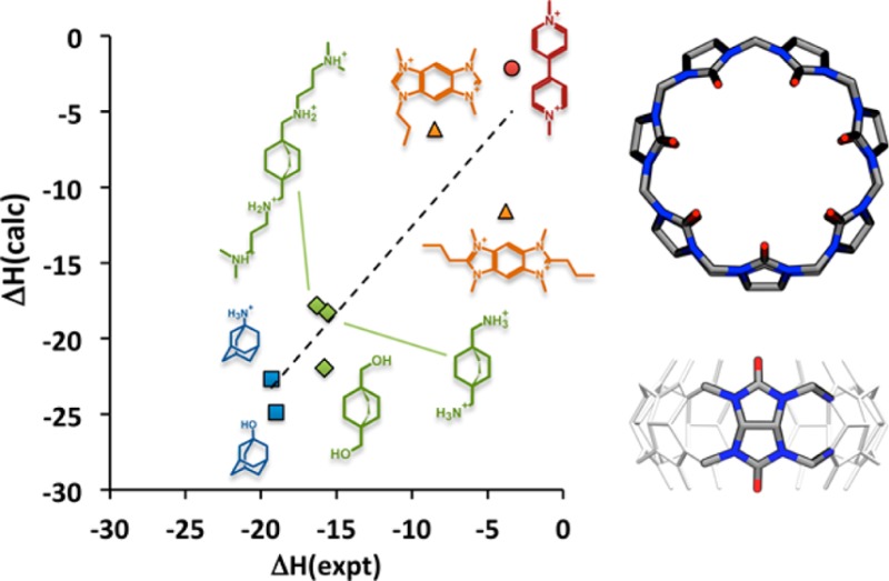
We used microsecond time scale molecular dynamics simulations, with explicit solvent comprising water and dissolved ions, to compute the binding enthalpies for the synthetic host CB7 with eight guest molecules (Figure 1). The experimental binding enthalpies, ΔH, correlate with the guests’ structural scaffolds: the most exothermic are the adamantanes (A1, A2),21 followed by the bicyclo[2.2.2]octanes (B2, B5, B11),21 the benzo-bis(imidazoles) (G8, G9),33 and finally methylviologen.34 The following subsections compare the computations with experiment and use energy decomposition analysis to study the physical determinants of these host–guest binding enthalpies.
Figure 1.
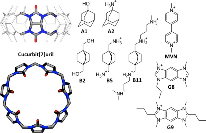
Structures of the host CB7 (left) and eight guest molecules for which binding enthalpies were computed here.
Comparison of Calculation with Experiment
Binding enthalpies computed with the TIP3P35 water model (Table 1) correlate well with experiment (Figure 2): linear regression analysis yields a correlation coefficient R = 0.91 ± 0.01, a slope near unity (1.15 ± 0.02), and a small y-intercept (−1.12 ± 0.21). There is a modest tendency to overestimate the binding enthalpies, indicated by a mean signed error (MSE) of −2.97 ± 0.09 kcal/mol across all eight guests. The calculations furthermore capture the physical interactions in the systems well enough to replicate the ranking of enthalpies according to the guests’ structural features, as indicated by the color-coding of data points in Figure 2. Matched simulations using the TIP4P-Ew36 water model, instead of TIP3P, also correlate well with experiment (R = 0.87 ± 0.01, slope 1.03 ± 0.02, y-intercept −6.35 ± 0.24) but further overestimate the measured affinities (MSE −6.75 ± 0.11 kcal/mol). Therefore, the energy decomposition studies that follow focus on the TIP3P results. However, the trends discussed here are consistent for TIP4P-Ew, as detailed in the SI.
Table 1. Binding Enthalpies (kcal/mol) and Associated Uncertainties from Experiment21,33,34 and Computation with Water Models TIP3P and TIP4P-Ew, As Noted.
| guest | ΔH (expt) | ΔH (calc,TIP3P) | ΔH (calc,TIP4P-Ew) |
|---|---|---|---|
| A1 | –19.0 ± 0.2 | –24.9 ± 0.2 | –25.4 ± 0.2 |
| A2 | –19.3 ± 0.2 | –22.7 ± 0.2 | –24.6 ± 0.2 |
| B2 | –15.8 ± 0.1 | –21.9 ± 0.2 | –23.9 ± 0.2 |
| B5 | –15.6 ± 0.2 | –18.3 ± 0.2 | –23.5 ± 0.2 |
| B11 | –16.3 ± 0.2 | –17.8 ± 0.2 | –24.3 ± 0.3 |
| G8 | –8.5 ± 0.3 | –6.2 ± 0.2 | –11.4 ± 0.2 |
| G9 | –3.8 ± 0.1 | –11.6 ± 0.2 | –17.4 ± 0.2 |
| MVN/Tris | –3.4 ± 0.2 | –2.1 ± 0.2 | –4.7 ± 0.2 |
Figure 2.
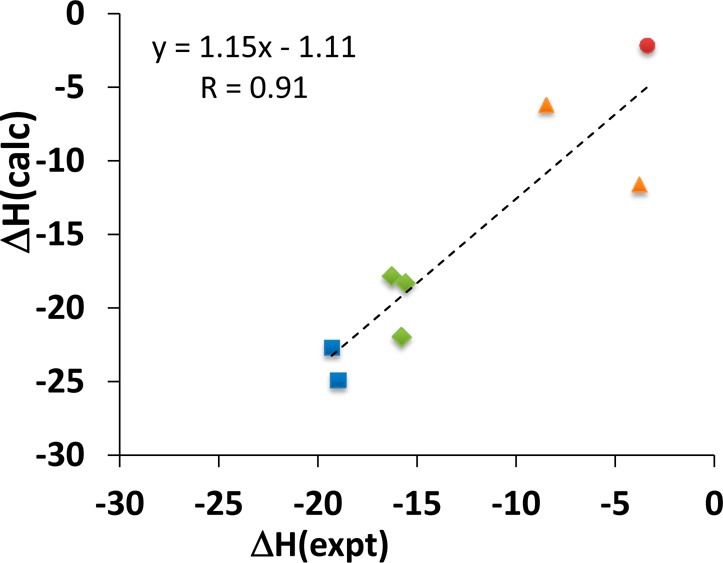
Comparison of binding enthalpies (kcal/mol) from experiment (expt) and simulation with TIP3P water model (calc), for CB7 with eight guest molecules. Blue squares: adamantyl derivatives, A1, A2. Green diamonds: bicyclo[2.2.2]octane derivatives: B2, B5. Orange triangles: G8, G9. Red circle: MVN (Tris included in simulation).
In assessing these results, it is essential to consider the uncertainties associated with both the computational and experimental results. As shown in Table 1, the reported experimental uncertainties of the mean range between 0.1 and 0.3 kcal/mol, and the numerical uncertainties of the computed enthalpies, based on blocking analysis (see Methods and SI), are commensurate, at 0.2 to 0.3 kcal/mol. (Note, we report standard deviations of the mean as our measure of computational uncertainty. Thus, to compare directly with experiment, we converted all previously reported experimental uncertainty values into standard deviations of the mean by dividing by the square root of the number of replicates.) The high precision of these calculations is supported by the fact that the correlation times estimated by blocking and statistical inefficiency analysis are at most 1.0 ps (see SI); therefore, each microsecond-duration simulation provided a minimum of ∼500 000 independent estimates of the mean energy. In addition, geometric analysis (see SI) shows that the guests thoroughly sample rotations about the symmetry axis of the CB7 host; and although the overall orientation of the guests within the host (“head in” versus “head out”) does not change during the simulations, sampling such reversals is not required to achieve convergence, because both orientations are chemically equivalent, due to the symmetry of CB7. The small uncertainties in the computational and experimental data lead to the correspondingly small uncertainties in the regression parameters reported above, based on bootstrap resampling of the experimental and computed enthalpies (see Methods).
We also determined the best agreement that could possibly be obtained with calculations at the present level of numerical precision, by imagining calculations which correctly yield the experimental binding enthalpies, but still with a numerical uncertainty of 0.2–0.3 kcal/mol (Table 1). Bootstrap resampling of data from this imagined computational study, and from the experimental data set with its own uncertainties, yields R = 1.00 ± 0.00, slope 1.00 ± 0.02, y-intercept −0.01 ± 0.23 kcal/mol, and MSE 0.00 ± 0.10 kcal/mol. The high quality of these idealized statistics suggest that the experimental and numerical precision are good enough that deficiencies in the simulation force field now represent the only obstacle to obtaining clear-cut agreement with experiment.
Physical Determinants of Binding Enthalpies
The present computational methodology enables informative decompositions of the binding enthalpy into energy components, and these components can furthermore be correlated with conformational preferences observed in the simulations. In this section, we use these capabilities to seek insight into the determinants of the observed binding enthalpies for the eight cucurbituril–guest systems.
van der Waals Interactions, Electrostatics, and the Role of Solvent
Table 2 provides a breakdown of binding enthalpies for all eight guests, computed with the TIP3P water model, into three contributions: one from the net change in the Lennard-Jones force field term, which primarily models van der Waals forces; one from the net change in Coulombic electrostatic interactions; and one from changes in valence terms, which comprise bond-stretch, bond-angle, and dihedral terms.
Table 2. Analysis of Binding Enthalpies (kcal/mol) Computed with the TIP3P Water Modela.
| ΔH (calc) |
||||||
|---|---|---|---|---|---|---|
| guest | tot | LJ | elec | val | charge | ΔNclose |
| A1 | –24.9 | –15.2 | –7.3 | –2.3 | 0 | 247 |
| A2 | –22.7 | –17.3 | –3.3 | –2.1 | 1 | 255 |
| B2 | –21.9 | –13.1 | –7.6 | –1.3 | 0 | 215 |
| B5 | –18.3 | –15.3 | –2.6 | –0.3 | 2 | 229 |
| B11 | –17.8 | –18.4 | 0.3 | 0.3 | 4 | 256 |
| G8 | –6.2 | –14.8 | 4.3 | 4.4 | 2 | 186 |
| G9 | –11.6 | –14.6 | 0.3 | 2.7 | 2 | 200 |
| MVN/Tris | –2.1 | 4.6 | –7.6 | 0.9 | 2 | –242 |
| MVN/noTris | –4.7 | –7.3 | 0.3 | 2.3 | 2 | 26 |
Tot: total computed enthalpy change on binding. LJ: Lennard-Jones contribution. Elec: Coulombic electrostatic contribution. Val: contribution from changes in bond-stretch, angle-bend, and dihedral terms. Charge: net charge of the guest (e). Nclose: change on binding in the number of atoms, solute or solvent, within 4.25 Å of any atom of the host and guest.
It is immediately noticeable that the Lennard-Jones term is consistently favorable (negative), except in the case of the methylviologen (MVN/Tris). The unique feature of the MVN system is the use of an organic buffer, Tris, which was included not only in the experiments but also in these initial methylviologen simulations (see Methods). It was therefore of interest to rerun the enthalpy calculation for MVN without Tris. The resulting binding enthalpy is more favorable by −2.6 kcal/mol, and the Lennard-Jones contribution is now favorable, similar to that of the other guests; see MVN/noTris in Table 2. Examination of the simulations in the presence of Tris reveals that this cationic compound takes up residence in the binding cavity of the free CB7 host (Figure 3) and is necessarily displaced when methylviologen binds. The consequent loss of favorable Lennard-Jones interactions between the Tris molecule and the host helps balance the gain in Lennard-Jones interactions between the guest and host, which is further discussed below.
Figure 3.
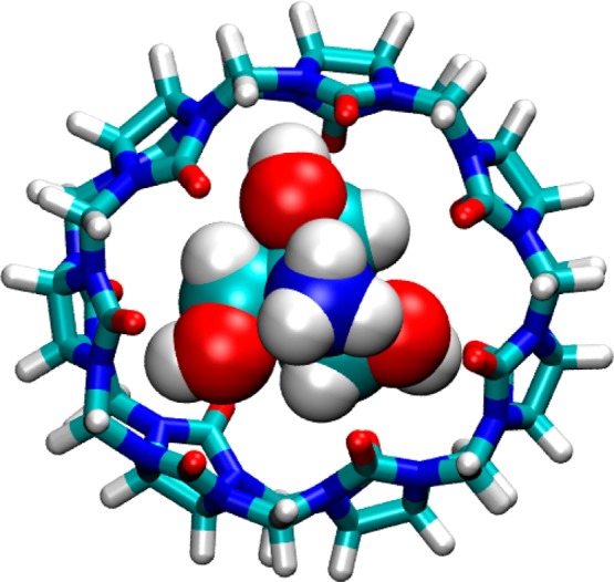
Representative conformation from simulation of CB7 host containing a molecule of Tris buffer (MVN/Tris).
Unlike the Lennard-Jones contribution, which is uniformly favorable in the absence of Tris, the electrostatic contribution varies in sign and tends to be smaller in magnitude (Table 2). Interestingly, when the TIP3P water model is used, the electrostatic contribution is anticorrelated with the charge of the guest, especially if the MVN/tris and G8 data are removed (see Table 2). However, there is little correlation between the electrostatic component and the charge of the guest when the TIP4P-Ew water model is used (see SI, Table S2). Further decomposition of the electrostatic contribution into solute and solvent parts reveals that its small and variable character results from systematic compensation of solute–solute interactions by changes in solvent electrostatics. Thus, as shown in the left panel of Figure 4, the net solvent contribution to the electrostatic contribution (green symbols) almost exactly cancels the strongly favorable solute–solute contributions (x-axis). Indeed, a linear regression fit gives y = −1.04x – 6.52 kcal/mol, with R = 1.00. Decomposition of the solvent contribution itself reveals strongly unfavorable losses in solute–solvent electrostatics on binding (blue symbols; y = −1.96x + 5.93 kcal/mol, R = 1.00) and favorable gains in solvent–solvent interactions (red symbols; y = 0.92x – 12.45, R = 0.98). Thus, although the host–guest electrostatic interactions range to almost −180 kcal/mol (Figure 4, left), they are almost perfectly balanced by compensating interactions involving the solvent: for every −1 kcal/mol of solute–solute electrostatic energy, there is a penalty of about +2 kcal/mol in solute–solvent energy, and a gain of about −1 kcal/mol of solvent–solvent energy. These powerful trends are consistent with the well-known concept that forming a new hydrogen-bond between two solutes in water requires sacrificing two solute-water hydrogen bonds, but also leads to the formation of one new water–water hydrogen bond between the released water molecules.
Figure 4.
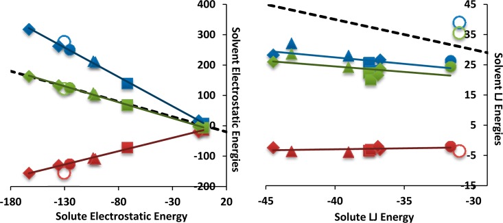
Role of solvent in electrostatic and Lennard-Jones interaction energies (kcal/mol). The shapes coincide with the same guests as shown in Figure 2. Solid green: net solvent contribution (solute–solvent + solvent–solvent). Solid blue: solute–solvent. Solid red: solvent–solvent contribution. The methylviologen calculations used for the trend lines exclude Tris. The methylviologen data points with Tris are shown as unfilled. Total cancellation between the net solvent effect and the solute–solute interaction energy is depicted as a dashed line, with a slope of −1.
Such strong solvent compensation is not observed for the Lennard-Jones contribution (Figure 4, right). Although the net solvent contributions to the Lennard-Jones term are unfavorable by roughly 25 kcal/mol, they do not fully cancel the solute–solute contribution, except in the special case of MVN/Tris (unfilled, green circle), where the solvent includes a molecule of Tris. Moreover, there is only a weak trend for the net solvent contribution to become more unfavorable as the solute–solute Lennard-Jones interaction becomes more favorable. One may conclude that the new solute–solute interactions formed on binding are stronger than the solute–solvent interactions that were sacrificed (blue symbols), and little solvent–solvent Lennard-Jones energy is recovered by water release (red symbols). As a consequence, much of the favorable solute–solute interaction remains in effect, leading to the favorable overall Lennard-Jones interactions listed in Table 2.
The fact that the solute–solute (i.e., host–guest) Lennard-Jones interactions formed on binding come at a relatively modest cost in solvent Lennard-Jones interactions may be attributed to the high packing density of atoms in the host–guest complex, relative to that of the water. The mesh of covalent bonds within the host and guest molecules means that there are more non-hydrogen atoms per unit volume than in liquid water, with its comparatively long interoxygen distances. As a consequence, binding increases the number of short-ranged (<4.25 Å) atom–atom interactions (Nclose in Table 2), except for MVN/Tris, and hence also increases the number of favorable Lennard-Jones interactions. This interpretation is supported by the correlation (R2 = 0.98) between Nclose and the net Lennard-Jones contribution to the binding enthalpy.
Aromatic versus Aliphatic Guests
The measured binding enthalpies of the three aromatic guests (G8, G9, and methylviologen) are notably less favorable than those of the five aliphatic guests (A1, A2, B2, B5, and B11). The calculations capture this experimental trend (Table 1 and Figure 2) and may be analyzed to seek a possible explanation for it. Because all three aromatic guests are dications, we compare them with the one cationic aliphatic guest, B5.
Although one might expect the aromatic, and hence relatively polarizable, methylviologen guest to form more favorable dispersion interactions with the CB7 host, relative to the aliphatic B5, its overall Lennard-Jones contribution is far less favorable, even when Tris is not included in the simulations (Table 2). This difference, along with more modest electrostatic and valence contributions, accounts for the less favorable binding overall enthalpy computed for MVN/noTris relative to B5. These differences are rationalized, at least in part, by comparison of representative structures of B5 and methylviologen complexed with CB7 (Figure 5). In particular, whereas the round bicyclo[2.2.2]octane core of B5 nicely fills the round cavity of CB7, the relatively flat core of methylviologen does not fit well. The unfilled gaps between this guest and the host correlate with the less favorable Lennard-Jones term, and the distortion of the normally circular host to an elliptical shape accounts for the valence penalty. In addition the net electrostatic contribution to the binding enthalpy of methylviologen is not favorable, when Tris is absent. This may reflect a combination of partial desolvation of its relatively delocalized positive charge, and its inability to donate hydrogen bonds to the carbonyl groups at the portal of CB7.
Figure 5.
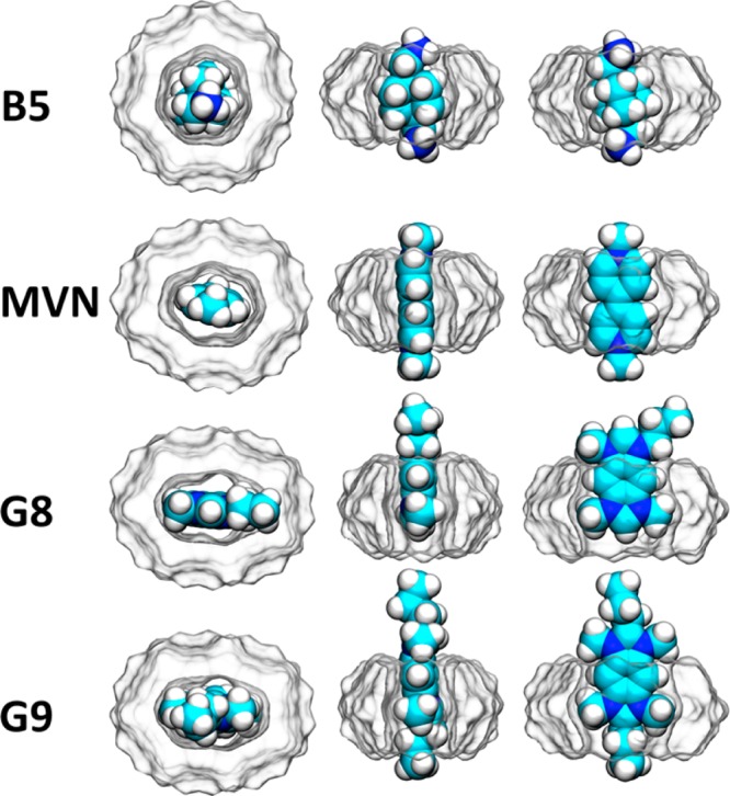
Representative conformations from the most probable cluster based on RMSD37 of the complexes of the dicationic guests B5, G8, G9, and MVN (space-filling representation) bound to CB7 (solvent-accessible surface representation), each shown from three viewpoints. Rendered with the program VMD.38
Interestingly, the pattern is somewhat different for the other two aromatic guests, G8 and G9. These maintain strongly favorable Lennard-Jones interactions with the host, despite their flattened shape, apparently because their methyl groups, absent in methylviologen, tuck neatly into equatorial grooves of the distorted CB7 host (Figure 5). In addition, the more elongated shape adopted by CB7 when G8 and G9 are bound may allow closer packing along the flat faces of these guests. However, the enthalpy decompositions of these two guests resemble methylviologen in the sense that they also do not have favorable net electrostatic contributions.
Discussion
Physical Basis of Aqueous Host–Guest Binding Enthalpies
The attractive component of the Lennard-Jones energy term, which accounts primarily for dispersion forces, contributes strongly to the computed binding enthalpies in all cases studied here, except in the special case where the organic buffer Tris is present in solution. The conclusion that dispersion interactions contribute strongly and consistently to the binding enthalpies may appear contrary to an elegant experimental study,39 which suggested that dispersion interactions contribute minimally to the folding free energy of a molecular torsion balance40 in various solvents. The authors argue that the favorable solute–solute dispersion interactions formed upon folding are closely balanced by simultaneous unfavorable losses in solute–solvent interactions. In the present calculations, too, the net dispersion interaction is a balance of solute–solute and solvent terms, but there is only partial cancellation by solvent, so the net dispersion contribution is strongly favorable. This result is explained by the increased number of close atom pairs for the complex versus the free host and guest, which in turn traces to the high packing density of the polycyclic host and guest molecules, relative to liquid water. The rigidity and the close fit of these complexes also presumably play a role. In contrast, for the torsion balance study, the interacting species in the torsion balance study are hexyl chains, which are much more flexible and less densely packed than the polycyclic molecules considered here. The relatively poor packing of these hexyl chains may well account for the modest contribution of dispersion forces to their association.
Another probing study41 used the correlation of a spectroscopic feature with solvent polarizability to suggest that the binding site of CB7 is of especially low polarizability, and argued on this basis that dispersion forces, which are closely related to electronic polarizability, play little role in the binding of guests by CB7. However, because the net contribution of dispersion interactions to the binding enthalpy is a balance between newly formed host–guest interactions and lost solute–water interactions, the net effect of a low polarizability binding cavity is hard to predict. Put differently, even if the CB7 host forms only weak dispersion interactions with the molecules in its binding cavity, it also loses only weak dispersion interactions with the water ejected from the cavity upon binding. As a consequence, the net change in dispersion energy could still be favorable.
A robust trend in the present experimental data is that the aromatic guests bind less enthalpically than the aliphatic ones; recent results for the guest berberine fit this pattern as well.42 Decomposition of the binding enthalpies into Lennard-Jones, electrostatic, and valence contributions, along with inspection of the structures of the complexes, suggests that this difference can be explained primarily by considerations of shape complementarity and electrostatics. Thus, the rounded bicyclooctane and adamantane cores of the aliphatic guests fit well into the preferred circular shape of the host, while positioning their polar groups outside the binding cavity and forming hydrogen bonds with host carbonyls. In contrast, the flatter aromatics distort the host and pay large electrostatic desolvation penalties that are not outweighed by favorable host–guest electrostatic interactions.
Implications for the Evaluation and Improvement of Simulation Force Fields
The TIP3P water model yields clearly more accurate results than TIP4P-Ew in the present application, even though the two models provide similarly accurate small molecule hydration free energies.43 In addition, TIP4P-Ew more faithfully reproduces various water properties, such as the oxygen–oxygen radial distribution function of neat water,36 the preferred geometries of gas-phase water clusters,44 the hydration enthalpy of methane,45 and the hydration enthalpies of both hydrophobic and polar amino acid side chain analogs.46 The fact that TIP4P-Ew yields stronger electrostatic contributions to the binding enthalpies than TIP3P appears consistent with the fact that TIP4P-Ew water has a room temperature dielectric constant lower than that of TIP3P: 62.936 versus 96.9.47 However, more subtle factors may also contribute to the differences in results from these two models. For example, they may ascribe different thermodynamic properties to the water in the binding cavity of the host molecule.48 Whatever the explanation, the present results strongly suggest that a water model optimized for one type of application, such as replicating the properties of neat water, may not be optimal for another application, such as the study of host–guest binding. It would appear that water models should tested against actual binding data, if they are to be used in applications where binding is of central interest, such as computer-aided drug design.
More generally, the fact that tightly converged host–guest binding enthalpies can now be computed efficiently on a commodity computer means that binding enthalpies can be added to the experimental data set for testing and improving simulation force fields. The set of observables currently used for this purpose primarily comprises small molecule hydration free energies46,49−54 and properties of pure liquids,55,56 such as densities and heats of vaporization. Although this data set is valuable, it does not probe many of the noncovalent interactions important in drug discovery, and as noted above, it does not test the ability of water models to correctly handle confined environments, such as protein binding sites. Kirkwood–Buff approaches,57−61 and approaches based on the conformational preferences of proteins and nucleic acids usefully examine the critical balance between solute–solvent and solute–solute interactions but are still limited in chemical scope and do not address the problem of confined water. Experimentally and computationally tractable host–guest systems offer new possibilities to probe the accuracy with which force fields account for the interactions of varied functional groups and for the thermodynamics of water in concave binding sites.48
Toward Computational Calorimetry
Although there are a number of computational techniques for estimating enthalpy changes,25,26,29 obtaining tightly converged binding enthalpies from simulations has been technically challenging. The present study demonstrates that microsecond simulations of host–guest systems, which are now readily achievable with GPU technology,31,32 can provide computed binding enthalpies with a precision comparable to the corresponding experimental uncertainties. We used the direct approach, which involves simulations only of the system’s initial and final states. Most other enthalpy methods require multiple simulations at stages along a pathway leading from the initial to the final state. For example, the finite difference (FD) method uses a pathway approach to compute the binding free energy at multiple temperatures, and then estimates the binding entropy, and hence enthalpy, from the temperature derivative of the free energy. Which of the various methods will be most numerically efficient likely depends upon the nature of the system being simulated. For example, the FD method may be preferable for large systems, where large energy fluctuations slow convergence of the direct method. On the other hand, the numerical properties of the direct method may be preferable for systems where the change in enthalpy is large,25,26,29,30 and its technical simplicity also is appealing. It should also be emphasized that the direct enthalpy method has the particular advantage of providing informative decompositions of the binding enthalpy, which may furthermore be connected with conformational preferences, as illustrated by the present study. It is not clear that other enthalpy methods can support such analyses.
Thus, the present study establishes that detailed atomistic simulations can provide tightly converged estimates of noncovalent binding enthalpies for molecular systems in aqueous solution, and can be used to seek explanations for calorimetric characterizations of binding. This is an important direction, because calorimetric data are often puzzling or even paradoxical.62,16 For example, small changes in chemical structure often lead to correspondingly small changes in free energy, but seemingly disproportionately large changes in enthalpy and entropy.8−13 Similarly, the efforts of medicinal chemists to enhance binding by making ligands more rigid, and thereby presumably reducing the entropy penalty, sometimes enhances the binding enthalpy instead of the entropy.14,15,23 The ability to informatively decompose binding enthalpies, as done here, should help resolve such calorimetric paradoxes. Moreover, by combining an enthalpy calculation with a precise calculation of the binding free energy,63−67 one can immediately obtain the binding entropy, a quantity which has been notoriously difficult to obtain at high precision from simulations. Such analyses are in progress in our laboratory. We anticipate that continuing growth in computer power will likely make such computational calorimetry studies routine before long, not only for host–guest binding but also for more challenging biomolecular systems.
Methods
We compute the enthalpy of binding as the difference between the mean energies of four systems (Figure 6), where the two initial states are the free host and guest in aqueous solvent, and the final states are the complex in solvent as well as an amount of pure solvent that exactly balances the solvent of the initial and final states. Although this solvent-balance approach was reported previously,68 it was presented without derivation. The Theory subsection therefore derives this direct enthalpy method; the subsection entitled Computational Methods section then details the simulations and their analysis.
Figure 6.
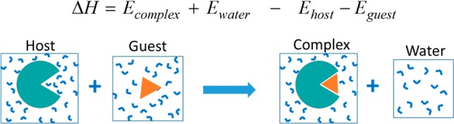
Solvent-balance method of computing binding enthalpies.
Theory of Solvent-Balance Binding Enthalpy Calculations
The standard free energy change on binding may be written in terms of the standard chemical potentials of the solvated reactant species, A, B and their product complex, AB:
| 1 |
The standard chemical potential of a solvated molecule or complex, X = A, B, or AB, at standard concentration in idealute solution is69
| 2 |
where R is the gas constant, C0 is the concentration at standard state conditions, and ZNX,X and ZNX,0 are the partition functions of NX water molecules with and without the solute, respectively. The symmetry number σX is included in case the partition function of X is written in a manner that includes indistinguishable conformations.70 We have omitted the momentum contribution to the partition function, as this will cancel when one assembles an expression for the standard free energy of binding from the chemical potential of the three molecular species. We also neglect a pressure–volume term, as its contribution to the binding enthalpy and free energy is negligibly small relative to the other terms in a solvated system.
The chemical potential μX0 is the partial molar free energy of species X = A, B, or AB and can be written in terms of the partial molar enthalpy hX and entropy sX: μX0 = hX – TsX. The binding enthalpy then is given by
| 3 |
One may use the fact that
| 4 |
to write the partial molar enthalpy as
| 5 |
Substituting eq 2 into eq 5 yields
| 6 |
The two partition functions here have the same basic form, Z = ∫ e–U(r)/RTdr, where U(r) is the potential energy of the system as a function of r, which comprises the coordinates of the solvent molecules as well as the solute, if present. It is straightforward to show that
| 7 |
where ⟨U⟩ is the Boltzmann average of the potential energy. Substituting eq 7 into eq 6 yields the partial molar enthalpy as
| 8 |
Here, the quantities in the angle brackets are the mean potential energies of the solute X with NX solvents, and of the NX solvent molecules without any solute, respectively. Finally, combining the partial molar enthalpies of the complex and the free solutes yields the desired enthalpy change on binding as
| 9 |
The first three terms here are the difference in the mean energy of the solute-water systems, and the last three terms are the mean energies of the waters from each system without the solutes. If dissolved ions, such as sodium and chloride, are present in any of the simulations with a solute present, then these must similarly be balanced between the initial and final states; see SI. Here, we evaluate the last term in eq 9 by computing the mean energy of a box of waters with (NAB – NA – NB) water molecules, along with a balancing set of ions as may be required.
Molecular Dynamics Simulations
The initial docked poses of the guests with CB7 were the lowest energy minima in a semiempirical quantum energy landscape as found via an aggressive conformational search.71 The GAFF72 force field was used for all the bonded and nonbonded parameters of CB7 and the guest molecules. Partial atomic charges were generated with the AM1-BCC73,74 method as implemented in the program Antechamber.75 Each system (free CB7, free guest, and CB7-guest) was then solvated with TIP3P35 and TIP4P-Ew36 explicit water molecules. Counter ions76 were added to neutralize the total charge of a given system. The ITC experiments associated with the aliphatic guests were done in “pure water”,21 but pH buffers were used in the experiments for the aromatic guests. The experiments involving methylviologen were done in the presence of 50 mM TRIS chloride at pH 7,34 which corresponds to 1.3 TRIS+ and Cl– ions in the volume of the simulation box, so one of each ionic species was included. The guests G8 and G9 were studied in 10 mM sodium phosphate buffer,33 which corresponds to only 0.3 phosphates and 0.4 sodiums in our simulation volumes, so these were not included. The number of explicit water molecules in each system was set such that the total number of waters in the bound state (complex and pure water simulations) and in the free state (CB7 and guest simulations) were equal. For each separate simulation, the orthorhombic box lengths were set equal in each spatial direction. A Langevin thermostat with the collision frequency set to 1.0 ps–1 was used for the NVT and NPT stages of equilibration, and the Berendsen barostat with the pressure set to 1 bar and the relaxation time set to 2 ps was used during the NPT stage of equilibration. Additional details on the minimization and equilibration protocols are given in the SI. Production NPT simulations used the same settings for the thermostat and barostat as during equilibration, except that the nonbonded cut off value was set to 9.0 Å. The first 10 ns of production simulation were discarded to allow for additional equilibration. The production simulation times were at least 1 μs for each system simulated (pure solvent, CB7, CB7–guest, and guests) for a total simulation time of over 38 μs across both water models.
Precise Calculation of Mean Potential Energies and Energy Components
We used the SANDER module of AMBER 1277 to recompute the potential energy for each trajectory snapshot when all the atoms are present (total), when only the solvent is present (solvent–solvent), and when only the solute is present (solute–solute). CPPTRAJ78 was used for the generation of all the modified topology and trajectory files necessary for the potential energy decomposition analysis. Convergence of the total potential energy was evaluated by plotting the cumulative average as a function the total simulation time, and by using block-averaging analysis79 to estimate the standard deviation of the mean potential energy. All reported average potential energies have a standard deviation of the mean of 0.13 kcal/mol or less (see SI); thus, if the same simulation were repeated multiple times, with different randomly assigned initial velocities, the standard deviation of the mean potential energy should be about 0.13 kcal/mol. The mean energies obtained for our pure water simulations are within 0.3 kcal/mol of published values.35,36 Because the binding enthalpy is an additive combination of four mean energies, the variances of the mean energies add, and the standard deviation of the mean binding enthalpy is given by σH = √Σi = 14σi, where σi is the standard deviation of the mean for simulation i.
Several variations of this protocol were run for one host–guest pair, CB7 with A2, to consider sources of error. First, one test calculation used NVT production runs, with box volumes set to the smallest or largest volume sampled from a prior NPT simulation of the same system. These extreme tests yielded binding enthalpies as much as 160 kcal/mol different from those obtained by otherwise identical NPT production runs. On the other hand, NVT calculations with the box volume set to the average obtained from the prior NPT calculation yielded results very similar to those from NPT production runs. We conclude that the mean energy is highly sensitive to the volume and that it is safest to use NPT conditions for enthalpy calculations. Therefore, all of the results reported here were obtained from NPT simulations. Second, because the default GPU implementation of AMBER employed here uses mixed precision arithmetic, we compared the results to those from matched simulations using full double precision on the GPU; the two results differed by only 0.09 kcal/mol. Finally, to address possible concerns regarding the use of a cutoff for Lennard-Jones interactions,80 we recomputed the energy of each snapshot for CB7 and A2, using the maximum cutoff value possible given the size of the simulation box. This change had minimal impact (0.07 kcal/mol) on the computed binding enthalpy. Further details are provided in the SI.
Linear Regression Analysis
The significance of the reported linear regression parameters and mean errors was assessed through bootstrap resampling (100 000 samples) of the computed and experimental binding enthalpies, based on their respective means and standard deviation of the mean. For the experimental data, the reported standard deviations divided by the square root of the number of independent runs were taken to be the reported uncertainties. Linear regressions were performed for each bootstrap sample, and we report the means, X, and standard deviations, σ, of the resulting regression parameters, in the form X ± σ.
Geometric Analysis of Near Atom-Pairs
The number of atoms close to the host and guest, Nclose, was calculated for all of the host, guest, and host–guest simulations using 100 000 frames (every 10 ps) from each 1 μs simulation via the “radial” command in CPPTRAJ.78 For a given simulation, all host–solvent, guest–solvent, and/or host–guest pairwise interactions within 4.25 Å were included in the average. Any self-pairwise interactions (e.g., host–host or guest–guest) were excluded from the average pairwise count.
Acknowledgments
We thank Dr. Ross C. Walker for helpful discussions regarding the Berendsen barostat implementation in the AMBER simulation package and Dr. William Swope for helpful discussions regarding the blocking analysis technique. M.K.G. has an equity interest in, and is a cofounder and scientific advisor of VeraChem LLC. This publication was supported by the National Institute of General Medical Sciences of the National Institutes of Health (NIH) Grant GM61300. These findings are solely of the authors and do not necessarily represent the views of the NIH.
Supporting Information Available
Alternative decomposition of the binding enthalpies based on solute–solute, solute–solvent, and solvent–solvent interactions; binding enthalpy results using the TIP4P-Ew water model; details on simulation convergence and estimation of the standard deviation of the means; sensitivity analysis to simulation ensemble parameters; derivation of binding enthalpy including the presence of counterions; and minimization and equilibration protocol for the molecular dynamics simulations. This material is available free of charge via the Internet at http://pubs.acs.org.
The authors declare no competing financial interest.
Funding Statement
National Institutes of Health, United States
Supplementary Material
References
- Wiseman T.; Williston S.; Brandts J. F.; Lin L.-N. Rapid Measurement of Binding Constants and Heats of Binding Using a New Titration Calorimeter. Anal. Biochem. 1989, 179, 131–137. [DOI] [PubMed] [Google Scholar]
- Talhout R.; Villa A.; Mark A. E.; Engberts J. B. F. N. Understanding Binding Affinity: A Combined Isothermal Titration Calorimetry/Molecular Dynamics Study of the Binding of a Series of Hydrophobically Modified Benzamidinium Chloride Inhibitors to Trypsin. J. Am. Chem. Soc. 2003, 125, 10570–10579. [DOI] [PubMed] [Google Scholar]
- Bissantz C.; Kuhn B.; Stahl M. A Medicinal Chemist’s Guide to Molecular Interactions. J. Med. Chem. 2010, 53, 5061–5084. [DOI] [PMC free article] [PubMed] [Google Scholar]
- Reynolds C. H.; Holloway M. K. Thermodynamics of Ligand Binding and Efficiency. ACS Med. Chem. Lett. 2011, 2, 433–437. [DOI] [PMC free article] [PubMed] [Google Scholar]
- Velázquez Campoy A.; Freire E. ITC in the Post-Genomic Era? Priceless. Biophys. Chem. 2005, 115, 115–124. [DOI] [PubMed] [Google Scholar]
- Freire E. Do Enthalpy and Entropy Distinguish First in Class from Best in Class?. Drug Discovery Today 2008, 13, 869–874. [DOI] [PMC free article] [PubMed] [Google Scholar]
- Ladbury J. E.; Klebe G.; Freire E. Adding Calorimetric Data to Decision Making in Lead Discovery: A Hot Tip. Nat. Rev. Drug Discovery 2010, 9, 23–27. [DOI] [PubMed] [Google Scholar]
- Lumry R.; Rajender S. Enthalpy–Entropy Compensation Phenomena in Water Solutions of Proteins and Small Molecules: A Ubiquitous Properly of Water. Biopolymers 1970, 9, 1125–1227. [DOI] [PubMed] [Google Scholar]
- Krug R. R.; Hunter W. G.; Grieger R. A. Statistical Interpretation of Enthalpy–Entropy Compensation. Nature 1976, 261, 566–567. [Google Scholar]
- Dunitz J. D. Win Some, Lose Some: Enthalpy–Entropy Compensation in Weak Intermolecular Interactions. Chem. Biol. 1995, 2, 709–712. [DOI] [PubMed] [Google Scholar]
- Sharp K. Entropy–Enthalpy Compensation: Fact or Artifact?. Protein Sci. 2001, 10, 661–667. [DOI] [PMC free article] [PubMed] [Google Scholar]
- Chodera J. D.; Mobley D. L. Entropy–Enthalpy Compensation: Role and Ramifications in Biomolecular Ligand Recognition and Design. Annu. Rev. Biophys. 2013, 42, 121–142. [DOI] [PMC free article] [PubMed] [Google Scholar]
- Fenley A. T.; Muddana H. S.; Gilson M. K. Entropy–Enthalpy Transduction Caused by Conformational Shifts Can Obscure the Forces Driving Protein–Ligand Binding. Proc. Natl. Acad. Sci. U.S.A. 2012, 109, 20006–20011. [DOI] [PMC free article] [PubMed] [Google Scholar]
- Udugamasooriya D. G.; Spaller M. R. Conformational Constraint in Protein Ligand Design and the Inconsistency of Binding Entropy. Biopolymers 2008, 89, 653–667. [DOI] [PubMed] [Google Scholar]
- Benfield A. P.; Teresk M. G.; Plake H. R.; DeLorbe J. E.; Millspaugh L. E.; Martin S. F. Ligand Preorganization May Be Accompanied by Entropic Penalties in Protein–Ligand Interactions. Angew. Chem., Int. Ed. 2006, 45, 6830–6835. [DOI] [PubMed] [Google Scholar]
- DeLorbe J. E.; Clements J. H.; Teresk M. G.; Benfield A. P.; Plake H. R.; Millspaugh L. E.; Martin S. F. Thermodynamic and Structural Effects of Conformational Constraints in Protein–Ligand Interactions. Entropic Paradoxy Associated with Ligand Preorganization. J. Am. Chem. Soc. 2009, 131, 16758–16770. [DOI] [PubMed] [Google Scholar]
- Rekharsky M. V.; Mori T.; Yang C.; Ko Y. H.; Selvapalam N.; Kim H.; Sobransingh D.; Kaifer A. E.; Liu S.; Isaacs L.; Chen W.; Moghaddam S.; Gilson M. K.; Kim K.; Inoue Y. A Synthetic Host–Guest System Achieves Avidin–Biotin Affinity by Overcoming Enthalpy–Entropy Compensation. Proc. Natl. Acad. Sci. U.S.A. 2007, 104, 20737–20742. [DOI] [PMC free article] [PubMed] [Google Scholar]
- Inoue Y.; Hakushi T.; Liu Y.; Tong L.; Shen B.; Jin D. Thermodynamics of Molecular Recognition by Cyclodextrins. 1. Calorimetric Titration of Inclusion Complexation of Naphthalenesulfonates with α-, β-, and γ-Cyclodextrins: Enthalpy–Entropy Compensation. J. Am. Chem. Soc. 1993, 115, 475–481. [Google Scholar]
- Rekharsky M.; Inoue Y. Chiral Recognition Thermodynamics of B-Cyclodextrin: The Thermodynamic Origin of Enantioselectivity and the Enthalpy–Entropy Compensation Effect. J. Am. Chem. Soc. 2000, 122, 4418–4435. [Google Scholar]
- Inoue Y.; Liu Y.; Tong L. H.; Shen B. J.; Jin D. S. Calorimetric Titration of Inclusion Complexation with Modified.beta.-Cyclodextrins. Enthalpy–Entropy Compensation in Host-Guest Complexation: From Ionophore to Cyclodextrin and Cyclophane. J. Am. Chem. Soc. 1993, 115, 10637–10644. [Google Scholar]
- Moghaddam S.; Yang C.; Rekharsky M.; Ko Y. H.; Kim K.; Inoue Y.; Gilson M. K. New Ultrahigh Affinity Host–Guest Complexes of Cucurbit[7]uril with Bicyclo[2.2.2]octane and Adamantane Guests: Thermodynamic Analysis and Evaluation of M2 Affinity Calculations. J. Am. Chem. Soc. 2011, 133, 3570–3581. [DOI] [PMC free article] [PubMed] [Google Scholar]
- Deng N.; Zhang P.; Cieplak P.; Lai L. Elucidating the Energetics of Entropically Driven Protein–Ligand Association: Calculations of Absolute Binding Free Energy and Entropy. J. Phys. Chem. B 2011, 115, 11902–11910. [DOI] [PMC free article] [PubMed] [Google Scholar]
- Shi Y.; Zhu C. Z.; Martin S. F.; Ren P. Probing the Effect of Conformational Constraint on Phosphorylated Ligand Binding to an SH2 Domain Using Polarizable Force Field Simulations. J. Phys. Chem. B 2012, 116, 1716–1727. [DOI] [PMC free article] [PubMed] [Google Scholar]
- Baron R.; Setny P.; Andrew McCammon J. Water in Cavity–Ligand Recognition. J. Am. Chem. Soc. 2010, 132, 12091–12097. [DOI] [PMC free article] [PubMed] [Google Scholar]
- Levy R. M.; Gallicchio E. Computer Simulations with Explicit Solvent: Recent Progress in the Thermodynamic Decomposition of Free Energies and in Modeling Electrostatic Effects. Annu. Rev. Phys. Chem. 1998, 49, 531–567. [DOI] [PubMed] [Google Scholar]
- Lu N.; Kofke D. A.; Woolf T. B. Staging Is More Important than Perturbation Method for Computation of Enthalpy and Entropy Changes in Complex Systems. J. Phys. Chem. B 2003, 107, 5598–5611. [Google Scholar]
- Peter C.; Oostenbrink C.; van Dorp A.; van Gunsteren W. F. Estimating Entropies from Molecular Dynamics Simulations. J. Chem. Phys. 2004, 120, 2652–2661. [DOI] [PubMed] [Google Scholar]
- Wan S.; Stote R. H.; Karplus M. Calculation of the Aqueous Solvation Energy and Entropy, as Well as Free Energy, of Simple Polar Solutes. J. Chem. Phys. 2004, 121, 9539–9548. [DOI] [PubMed] [Google Scholar]
- Wyczalkowski M. A.; Vitalis A.; Pappu R. V. New Estimators for Calculating Solvation Entropy and Enthalpy and Comparative Assessments of Their Accuracy and Precision. J. Phys. Chem. B 2010, 114, 8166–8180. [DOI] [PubMed] [Google Scholar]
- Roy A.; Hua D. P.; Ward J. M.; Post C. B. Relative Binding Enthalpies from Molecular Dynamics Simulations Using a Direct Method. J. Chem. Theory Comput. 2014, 1072759–2768 10.1021/ct500200n. [DOI] [PMC free article] [PubMed] [Google Scholar]
- Lai B.; Oostenbrink C. Binding Free Energy, Energy and Entropy Calculations Using Simple Model Systems. Theor. Chem. Acc. 2012, 131, 1–13. [Google Scholar]
- Le Grand S.; Götz A. W.; Walker R. C. SPFP: Speed without Compromise—A Mixed Precision Model for GPU Accelerated Molecular Dynamics Simulations. Comput. Phys. Commun. 2013, 184, 374–380. [Google Scholar]
- Salomon-Ferrer R.; Götz A. W.; Poole D.; Le Grand S.; Walker R. C. Routine Microsecond Molecular Dynamics Simulations with AMBER on GPUs. 2. Explicit Solvent Particle Mesh Ewald. J. Chem. Theory Comput. 2013, 9, 3878. [DOI] [PubMed] [Google Scholar]
- Muddana H. S.; Varnado C. D.; Bielawski C. W.; Urbach A. R.; Isaacs L.; Geballe M. T.; Gilson M. K. Blind Prediction of Host–Guest Binding Affinities: A New SAMPL3 Challenge. J. Comput.-Aided Mol. Des. 2012, 26, 475–487. [DOI] [PMC free article] [PubMed] [Google Scholar]
- Kim H.-J.; Jeon W. S.; Ko Y. H.; Kim K. Inclusion of Methylviologen in Cucurbit[7]uril. Proc. Natl. Acad. Sci. U.S.A. 2002, 99, 5007–5011. [DOI] [PMC free article] [PubMed] [Google Scholar]
- Jorgensen W. L.; Chandrasekhar J.; Madura J. D.; Impey R. W.; Klein M. L. Comparison of Simple Potential Functions for Simulating Liquid Water. J. Chem. Phys. 1983, 79, 926–935. [Google Scholar]
- Horn H. W.; Swope W. C.; Pitera J. W.; Madura J. D.; Dick T. J.; Hura G. L.; Head-Gordon T. Development of an Improved Four-Site Water Model for Biomolecular Simulations: TIP4P-Ew. J. Chem. Phys. 2004, 120, 9665. [DOI] [PubMed] [Google Scholar]
- Shao J.; Tanner S. W.; Thompson N.; Cheatham T. E. Clustering Molecular Dynamics Trajectories: 1. Characterizing the Performance of Different Clustering Algorithms. J. Chem. Theory Comput. 2007, 3, 2312–2334. [DOI] [PubMed] [Google Scholar]
- Humphrey W.; Dalke A.; Schulten K. VMD: Visual Molecular Dynamics. J. Mol. Graph. 1996, 14, 33–38. [DOI] [PubMed] [Google Scholar]
- Yang L.; Adam C.; Nichol G. S.; Cockroft S. L. How Much Do van Der Waals Dispersion Forces Contribute to Molecular Recognition in Solution?. Nat. Chem. 2013, 5, 1006–1010. [DOI] [PubMed] [Google Scholar]
- Paliwal S.; Geib S.; Wilcox C. S. Molecular Torsion Balance for Weak Molecular Recognition Forces. Effects of “Tilted-T” Edge-to-Face Aromatic Interactions on Conformational Selection and Solid-State Structure. J. Am. Chem. Soc. 1994, 116, 4497–4498. [Google Scholar]
- Marquez C.; Nau W. M. Polarizabilities Inside Molecular Containers. Angew. Chem., Int. Ed. 2001, 40, 4387–4390. [DOI] [PubMed] [Google Scholar]
- Miskolczy Z.; Biczók L. Kinetics and Thermodynamics of Berberine Inclusion in Cucurbit[7]uril. J. Phys. Chem. B 2014, 118, 2499. [DOI] [PubMed] [Google Scholar]
- Klimovich P. V.; Mobley D. L. Predicting Hydration Free Energies Using All-Atom Molecular Dynamics Simulations and Multiple Starting Conformations. J. Comput.-Aided Mol. Des. 2010, 24, 307–316. [DOI] [PubMed] [Google Scholar]
- Kiss P. T.; Baranyai A. Sources of the Deficiencies in the Popular SPC/E and TIP3P Models of Water. J. Chem. Phys. 2011, 134, 054106. [DOI] [PubMed] [Google Scholar]
- Ashbaugh H. S.; Collett N. J.; Hatch H. W.; Staton J. A. Assessing the Thermodynamic Signatures of Hydrophobic Hydration for Several Common Water Models. J. Chem. Phys. 2010, 132, 124504. [DOI] [PubMed] [Google Scholar]
- Hess B.; van der Vegt N. F. A. Hydration Thermodynamic Properties of Amino Acid Analogues: A Systematic Comparison of Biomolecular Force Fields and Water Models. J. Phys. Chem. B 2006, 110, 17616–17626. [DOI] [PubMed] [Google Scholar]
- Höchtl P.; Boresch S.; Bitomsky W.; Steinhauser O. Rationalization of the Dielectric Properties of Common Three-Site Water Models in Terms of Their Force Field Parameters. J. Chem. Phys. 1998, 109, 4927–4937. [Google Scholar]
- Nguyen C. N.; Young T. K.; Gilson M. K. Grid Inhomogeneous Solvation Theory: Hydration Structure and Thermodynamics of the Miniature Receptor cucurbit[7]uril. J. Chem. Phys. 2012, 137, 044101. [DOI] [PMC free article] [PubMed] [Google Scholar]
- Nicholls A.; Mobley D. L.; Guthrie J. P.; Chodera J. D.; Bayly C. I.; Cooper M. D.; Pande V. S. Predicting Small-Molecule Solvation Free Energies: An Informal Blind Test for Computational Chemistry. J. Med. Chem. 2008, 51, 769–779. [DOI] [PubMed] [Google Scholar]
- Mobley D. L.; Dumont É.; Chodera J. D.; Dill K. A. Comparison of Charge Models for Fixed-Charge Force Fields: Small-Molecule Hydration Free Energies in Explicit Solvent. J. Phys. Chem. B 2007, 111, 2242–2254. [DOI] [PubMed] [Google Scholar]
- Mobley D. L.; Wymer K. L.; Lim N. M.; Guthrie J. P.. Blind Prediction of Solvation Free Energies from the SAMPL4 Challenge. J. Comput.-Aided Mol. Des. 1–16. [DOI] [PMC free article] [PubMed] [Google Scholar]
- Mobley D. L.; Bayly C. I.; Cooper M. D.; Shirts M. R.; Dill K. A. Small Molecule Hydration Free Energies in Explicit Solvent: An Extensive Test of Fixed-Charge Atomistic Simulations. J. Chem. Theory Comput. 2009, 5, 350–358. [DOI] [PMC free article] [PubMed] [Google Scholar]
- Guthrie J. P. A Blind Challenge for Computational Solvation Free Energies: Introduction and Overview. J. Phys. Chem. B 2009, 113, 4501–4507. [DOI] [PubMed] [Google Scholar]
- Geballe M. T.; Skillman A. G.; Nicholls A.; Guthrie J. P.; Taylor P. J. The SAMPL2 Blind Prediction Challenge: Introduction and Overview. J. Comput.-Aided Mol. Des. 2010, 24, 259–279. [DOI] [PubMed] [Google Scholar]
- Jorgensen W. L.; Maxwell D. S.; Tirado-Rives J. Development and Testing of the OPLS All-Atom Force Field on Conformational Energetics and Properties of Organic Liquids. J. Am. Chem. Soc. 1996, 118, 11225–11236. [Google Scholar]
- Chapman D. E.; Steck J. K.; Nerenberg P. S. Optimizing Protein–Protein van Der Waals Interactions for the AMBER ff9x/ff12 Force Field. J. Chem. Theory Comput. 2013, 10, 273–281. [DOI] [PubMed] [Google Scholar]
- Klasczyk B.; Knecht V. Kirkwood–Buff Derived Force Field for Alkali Chlorides in Simple Point Charge Water. J. Chem. Phys. 2010, 132, 024109. [DOI] [PubMed] [Google Scholar]
- Smith P. E. Chemical Potential Derivatives and Preferential Interaction Parameters in Biological Systems from Kirkwood–Buff Theory. Biophys. J. 2006, 91, 849–856. [DOI] [PMC free article] [PubMed] [Google Scholar]
- Gee M. B.; Smith P. E. Kirkwood–Buff Theory of Molecular and Protein Association, Aggregation, and Cellular Crowding. J. Chem. Phys. 2009, 131, 165101. [DOI] [PMC free article] [PubMed] [Google Scholar]
- Lin B.; Lopes P. E. M.; Roux B.; A D. M. Jr Kirkwood–Buff Analysis of Aqueous N-Methylacetamide and Acetamide Solutions Modeled by the CHARMM Additive and Drude Polarizable Force Fields. J. Chem. Phys. 2013, 139, 084509. [DOI] [PMC free article] [PubMed] [Google Scholar]
- Lin B.; He X.; MacKerell A. D. A Comparative Kirkwood–Buff Study of Aqueous Methanol Solutions Modeled by the CHARMM Additive and Drude Polarizable Force Fields. J. Phys. Chem. B 2013, 117, 10572–10580. [DOI] [PMC free article] [PubMed] [Google Scholar]
- Krishnamurthy V. M.; Bohall B. R.; Semetey V.; Whitesides G. M. The Paradoxical Thermodynamic Basis for the Interaction of Ethylene Glycol, Glycine, and Sarcosine Chains with Bovine Carbonic Anhydrase II: An Unexpected Manifestation of Enthalpy/Entropy Compensation. J. Am. Chem. Soc. 2006, 128, 5802–5812. [DOI] [PMC free article] [PubMed] [Google Scholar]
- Straatsma T. P.; McCammon J. A. Computational Alchemy. Annu. Rev. Phys. Chem. 1992, 43, 407–435. [Google Scholar]
- Gilson M. K.; Given J. A.; Bush B. L.; McCammon J. A. The Statistical-Thermodynamic Basis for Computation of Binding Affinities: A Critical Review. Biophys. J. 1997, 72, 1047–1069. [DOI] [PMC free article] [PubMed] [Google Scholar]
- Roux B. The Calculation of the Potential of Mean Force Using Computer Simulations. Comput. Phys. Commun. 1995, 91, 275–282. [Google Scholar]
- Woo H.-J.; Roux B. Calculation of Absolute Protein–Ligand Binding Free Energy from Computer Simulations. Proc. Natl. Acad. Sci. U.S.A. 2005, 102, 6825–6830. [DOI] [PMC free article] [PubMed] [Google Scholar]
- Velez-Vega C.; Gilson M. K. Overcoming Dissipation in the Calculation of Standard Binding Free Energies by Ligand Extraction. J. Comput. Chem. 2013, 34, 2360–2371. [DOI] [PMC free article] [PubMed] [Google Scholar]
- Sellner B.; Zifferer G.; Kornherr A.; Krois D.; Brinker U. H. Molecular Dynamics Simulations of B-Cyclodextrin-Aziadamantane Complexes in Water. J. Phys. Chem. B 2008, 112, 710–714. [DOI] [PubMed] [Google Scholar]
- Gilson M. K.; Given J. A.; Bush B. L.; McCammon J. A. The Statistical-Thermodynamic Basis for Computation of Binding Affinities: A Critical Review. Biophys. J. 1997, 72, 1047–1069. [DOI] [PMC free article] [PubMed] [Google Scholar]
- Gilson M. K.; Irikura K. K. Symmetry Numbers for Rigid, Flexible, and Fluxional Molecules: Theory and Applications. J. Phys. Chem. B 2010, 114, 16304–16317. [DOI] [PMC free article] [PubMed] [Google Scholar]
- Muddana H. S.; Gilson M. K. Calculation of Host–Guest Binding Affinities Using a Quantum-Mechanical Energy Model. J. Chem. Theory Comput. 2012, 8, 2023–2033. [DOI] [PMC free article] [PubMed] [Google Scholar]
- Wang J.; Wolf R. M.; Caldwell J. W.; Kollman P. A.; Case D. A. Development and Testing of a General Amber Force Field. J. Comput. Chem. 2004, 25, 1157–1174. [DOI] [PubMed] [Google Scholar]
- Jakalian A.; Bush B. L.; Jack D. B.; Bayly C. I. Fast, Efficient Generation of High-Quality Atomic Charges. AM1-BCC Model: I. Method. J. Comput. Chem. 2000, 21, 132–146. [DOI] [PubMed] [Google Scholar]
- Jakalian A.; Jack D. B.; Bayly C. I. Fast, Efficient Generation of High-Quality Atomic Charges. AM1-BCC Model: II. Parameterization and Validation. J. Comput. Chem. 2002, 23, 1623–1641. [DOI] [PubMed] [Google Scholar]
- Wang J.; Wang W.; Kollman P. A.; Case D. A. Automatic Atom Type and Bond Type Perception in Molecular Mechanical Calculations. J. Mol. Graph. Modell. 2006, 25, 247–260. [DOI] [PubMed] [Google Scholar]
- Joung I. S.; Cheatham T. E. Molecular Dynamics Simulations of the Dynamic and Energetic Properties of Alkali and Halide Ions Using Water-Model-Specific Ion Parameters. J. Phys. Chem. B 2009, 113, 13279–13290. [DOI] [PMC free article] [PubMed] [Google Scholar]
- Case D. A.; Darden T. A.; Cheatham T. E.; Simmerling C. L.; Wang J.; Duke R. E.; Luo R.; Walker R. C.; Zhang W.; Merz K. M.; Roberts B.; Hayik S.; Roitberg A.; Seabra J.; Swails J.; Goetz A. W.; Kolossváry I.; Wong K. F.; Paesani F.; Vanicek J.; Wolf R. M.; Liu J.; Wu X.; Brozell S. R.; Steinbrecher T.; Gohlke H.; Cai Q.; Ye X.; Wang J.; Hsieh M.-J.; Cui G.; Roe D. R.; Mathews D. H.; Seetin M. G.; Salomon-Ferrer R.; Sagui C.; Babin V.; Luchko T.; Gusarov S.; Kovalenko A.; Kollman P. A.. AMBER 12; University of California San Francisco: San Francisco, 2012.
- Roe D. R.; Cheatham T. E. PTRAJ and CPPTRAJ: Software for Processing and Analysis of Molecular Dynamics Trajectory Data. J. Chem. Theory Comput. 2013, 9, 3084–3095. [DOI] [PubMed] [Google Scholar]
- Flyvbjerg H.; Petersen H. G. Error Estimates on Averages of Correlated Data. J. Chem. Phys. 1989, 91, 461–466. [Google Scholar]
- Shirts M. R.; Mobley D. L.; Chodera J. D.; Pande V. S. Accurate and Efficient Corrections for Missing Dispersion Interactions in Molecular Simulations. J. Phys. Chem. B 2007, 111, 13052–13063. [DOI] [PubMed] [Google Scholar]
Associated Data
This section collects any data citations, data availability statements, or supplementary materials included in this article.