ROC curve inference for best linear combination of two biomarkers subject to limits of detection

Abstract

The receiver operating characteristic (ROC) curve is a tool commonly used to evaluate biomarker utility in clinical diagnosis of disease. Often, multiple biomarkers are developed to evaluate the discrimination for the same outcome. Levels of multiple biomarkers can be combined via best linear combination (BLC) such that their overall discriminatory ability is greater than any of them individually. Biomarker measurements frequently have undetectable levels below a detection limit sometimes denoted as limit of detection (LOD). Ignoring observations below the LOD or substituting some replacement value as a method of correction has been shown to lead to negatively biased estimates of the area under the ROC curve for some distributions of single biomarkers. In this paper, we develop asymptotically unbiased estimators, via the maximum likelihood technique, of the area under the ROC curve of BLC of two bivariate normally distributed biomarkers affected by LODs. We also propose confidence intervals for this area under curve. Point and confidence interval estimates are scrutinized by simulation study, recording bias and root mean square error and coverage probability, respectively. An example using polychlorinated biphenyl (PCB) levels to classify women with and without endometriosis illustrates the potential benefits of our methods.

1 Introduction

The use of biomarkers to assist medical decision making, the diagnosis and prognosis of individuals with a given disease, is increasingly common in both clinical settings and epidemiological research. This has spurred an increase in exploration for and development of new biomarkers. All biomarkers, established and emerging, are limited by the sensitivity of the measurement instrument which can lead to censored observations, often more frequently in emerging biomarkers as laboratory methods are underdeveloped. This censoring process is due to a limit of detection (LOD) or the inability of an instrument to reliably measure samples below (or in some cases above) some threshold. Polychlorinated biphenyl (PCB) levels fit this scenario well as they have been linked with several adverse outcomes and their measurements are affected by LODs. A common statistical tool used to evaluate the utility of a potential biomarker such as PCBs is the receiver operating characteristic (ROC) curve.

Consider populations of diseased and non-diseased people with levels of a specific biomarker denoted by independent random variables X and Y, respectively, with cumulative distribution functions F(x) and G(y). Suppose, the biomarker is utilized as an indicator of disease status where a level above some cut point, c, indicates a positive test for the disease and a level below c corresponds to a negative test. The sensitivity (the true positive test rate) and specificity (the true negative test rate) of the biomarker for a given c are q(c) = 1− F(c) and p(c) = G(c), respectively. The ROC curve is then a mapping of {1 − p(c), q(c)} across all possible c. Proposed uses for the ROC curve (Zhou et al., 2002; Pepe, 2003) include assessing discriminatory ability over all c, over a specific range of q(c) or p(c) and the maximum ability to differentiate between the populations. The area under the ROC curve, denoted here by AUC, is the most commonly used summary measure (Zhou et al., 2002; Pepe, 2003) and has been shown to be P(X>Y) for continuously measured biomarkers. AUC tends to range from 0.5 to 1 with larger values indicating greater separation between diseased and non-diseased biomarker levels. As a result, given multiple markers for the same disease, a researcher would be inclined to choose the one with the highest AUC to aid in decision making. Another approach would be to utilize a linear combination of these multiple biomarkers in lieu of selecting one. The attractiveness of a linear combination lies in being able to better discriminate, achieve a higher AUC, than if using any single biomarker alone.

Now consider the case where two biomarkers, X⃗ = (X₁, X₂)^T and Y⃗ = (Y₁, Y₂)^T, measured in individuals with and without a disease, respectively, are independent bivariate normally distributed. Clearly, each biomarker considered individually would be normally distributed and AUC’s for each could be calculated and contrasted. The alternative described previously would be to use a linear combination, say U = β⃗^T X⃗ = β₁ X₁ + β₂ X₂ and V = β⃗^T Y⃗ = β₁ Y₁+β₂ Y₂, as a composite “biomarker” for decision making. Conveniently, U and V are also normally distributed with an ROC curve that is now a function of the choice of β⃗^T and the corresponding AUC can be denoted by AUC_β.

Linear combinations for binary outcomes are often estimated using logistic regression for a given set of covariates. However, given this scenario of having several biomarkers following a multivariate normal distribution, Su and Liu (1993) developed a best linear combination (BLC), ${\overrightarrow{\mathrm{\beta }}}_0^{\mathrm{T}}$, leading to AUC₀, that is “best” with respect to maximizing AUC_β over all real β⃗^T directly rather than maximizing the logistic regression model which, can be concordant or discordant depending on the scenario (Pepe et al., 2006). This would allow for better discrimination than from any individual biomarker. When normal parameter values are unknown, we can use random samples to calculate estimates ${\widehat{\overrightarrow{\mathrm{\beta }}}}_0^{\mathrm{T}}$ and AÛC₀ via maximum likelihood techniques.

One common complication in biomarker evaluation is that for a variety of reasons, random samples X and Y of biomarkers are often evaluated with non-detects or missing data below some LOD, quantified as d, effectively censoring the data below d. Omitting these values and proceeding with a complete case analysis has been shown to lead to biased AÛC for univariate normal and gamma distributed biomarkers (Perkins et al., 2007). Categorizing the missing biomarker levels as ties at the lowest score, the standard non-parametric ROC curve and empirical AUC yield unbiased estimates of the biomarkers’ effectiveness given the measurement limitations. However, when underlying discriminatory ability is of interest, parametric methods can be used to estimate the ROC curve below the LOD and thus an AUC for a latent variable that might be measured completely. Generally, substituting a replacement value such as 0, d/2, $d/\sqrt{2}$ and d for unobservable data have been shown as a simple method to lessen biased parametric estimation (e.g. mean, variance and potential AUC) but the magnitude and direction of the remaining bias is highly dependent on the value chosen as well as the parameter being estimated (Hornung and Reed, 1990). It has been shown (Haas and Scheff, 1990; Lyles et al., 2001; Singh and Nocerino, 2002; Lynn, 2001; Perkins et al., 2007) that all of these methods lead to biased estimation of mean and standard deviation parameters, regression coefficients, odds ratio and AUC for a single biomarker following common distributions. In the logistic regression framework which has similarities here, Lynn (2001) demonstrated that the bias of these replacement values lessens the closer they are to the expected value below d, which performed similarly to more sophisticated methods of estimation.

Lyles et al. (2001) proposed a more thoughtful solution of constructing a likelihood function for two censored bivariate normally distributed random variables. Based on this likelihood and under the assumption of normality, subsequent maximum likelihood estimators (MLEs) are efficient and asymptotically unbiased point estimators.

In this paper, we propose in Section 2 to obtain MLEs for normal distribution parameters using Lyles et al.’s (2001) bivariate normal developments for parameter estimates based on a sample with left censoring in order to construct ${\widehat{\overrightarrow{\mathrm{\beta }}}}_0^{\mathrm{T}}$ and AÛC₀ to estimate that underlying potential of the BLC of two biomarkers. In Section 3, we extend Lyles et al. (2001) and consider the asymptotic distributions of parameter estimates by constructing the Fisher Information matrix for this case. Also in Section 3, these developments are subsequently used in finding the asymptotic distributions of point estimates ${\widehat{\overrightarrow{\mathrm{\beta }}}}_0^{\mathrm{T}}$ and AÛC₀, leading to accompanying confidence intervals (CIs). This procedure allows for the estimation of the BLC’s underlying discriminatory ability or the potential that could be realized if it were possible to eliminate the LOD and censoring in the tail. This would be especially useful when researchers are exploring biomarkers for a given outcome using more cost-effective but less-sensitive assays, with the idea of further measurements or re-measurement being conducted on a narrowed set of promising biomarkers using a more sensitive and costly, “gold standard” assay. When a more sensitive assay is lacking this would help identify biomarkers with potential that are worth additional resources in refining a measurement process. However, the discriminatory ability of the BLC of these biomarkers as measured with LOD is better estimated using the AUC for traditional empirical ROC curve, denoted AŨC₀ here, which appropriately accounts for the censored values by essentially treating them as ties because they are indiscernible from one another. In Section 4, simulation is used to assess ${\widehat{\overrightarrow{\mathrm{\beta }}}}_0^{\mathrm{T}}$ and point estimators AÛC₀ and AŨC₀ as well as CIs for AUC₀. An example in Section 5 using levels of the environmental toxicants PCBs to classify women with endometriosis is used to illustrate empirical and maximum likelihood techniques. We end with a brief discussion of issues surrounding estimation based on two biomarkers affected by LODs.

2 Methods

Suppose that pairs of biomarkers’ levels X⃗ = (X₁, X₂)^T and Y⃗ = (Y₁, Y₂)^T for cases and controls, respectively, are independent and have bivariate normal distributions f(X⃗; μ⃗_X, Σ_X) and g(Y⃗; μ⃗_Y, Σ_Y), respectively. These distributions can be written in a matrix form or explicitly expanded

$$\begin{array}{l}g(\overrightarrow{W};\overrightarrow{\mathrm{\mu }},\mathbf{\sum })=\frac{1}{2\mathrm{\pi }{\mid \mathbf{\sum }\mid }^{1/2}}exp\left\{-\frac{1}{2}{(\overrightarrow{W}-\overrightarrow{\mathrm{\mu }})}^{\mathrm{T}}{\mathbf{\sum }}^{-1}(\overrightarrow{W}-\overrightarrow{\mathrm{\mu }})\right\}\\ =\frac{1}{2\mathrm{\pi }{\mathrm{\sigma }}_1{\mathrm{\sigma }}_2\sqrt{1-{\mathrm{\rho }}^2}}exp\left\{-\frac{1}{2(1-{\mathrm{\rho }}^2)}({\mathrm{\eta }}_1^2-2\mathrm{\rho }{\mathrm{\eta }}_1{\mathrm{\eta }}_2+{\mathrm{\eta }}_2^2)\right\},\end{array}$$

where η_l = (w_l − μ_l)/σ_l, l = 1,2, μ⃗ = (μ₁, μ₂)^T is the mean vector and the covariance matrix Σ consists of variances, ${\mathrm{\sum }}_{ll}={\mathrm{\sigma }}_l^2$ and covariance terms, Σ₁₂ = Σ₂₁ = ρσ₁σ₂. For ease of development, we will exclusively work with the latter, explicit form. Under this assumption Su and Liu (1993) showed that the formulae for coefficients leading to the BLC’s ROC curve is

$${\overrightarrow{\mathrm{\beta }}}_0^{\mathrm{T}}\propto {({\overrightarrow{\mathrm{\mu }}}_X-{\overrightarrow{\mathrm{\mu }}}_Y)}^{\mathrm{T}}{({\mathbf{\sum }}_X+{\mathbf{\sum }}_Y)}^{-1},$$ (1)

which in turn leads to,

$${\text{AUC}}_0=\mathrm{P}(U>V)=\mathrm{\Phi }\left(\sqrt{{({\overrightarrow{\mathrm{\mu }}}_X-{\overrightarrow{\mathrm{\mu }}}_Y)}^{\mathrm{T}}{({\mathbf{\sum }}_X+{\mathbf{\sum }}_Y)}^{-1}({\overrightarrow{\mathrm{\mu }}}_X-{\overrightarrow{\mathrm{\mu }}}_Y)}\right).$$ (2)

Now suppose that the biomarker levels are measured with fixed LODs d⃗ = (d₁, d₂)^T. Let the measured observations, Z⃗_X and Z⃗_Y, be the componentwise transformation of X⃗ and Y⃗, respectively, such that

$$Z_{Xl}=\{\begin{array}{ll}{X}_l;\hfill & X_l\ge d_l,\hfill \\ N/A;\hfill & X_l<d_l,\hfill \end{array}\text{and}{Z}_{Yl}=\{\begin{array}{ll}{Y}_l;\hfill & Y_l\ge d_l,\hfill \\ N/A;\hfill & Y_l<d_l,\hfill \end{array}$$

where for a fixed d_l, l = 1, 2, the l-th biomarker level is either quantified or not. Without loss of generality we assumed that both diseased and non-diseased biomarker measurements were affected by the same point of censoring, say d_Xl = d_Yl = d_l.

Lyles et al. (2001) considered the case of two censored bivariate normally distributed random variables and developed the likelihood

$$\begin{array}{l}L(\overrightarrow{\mathrm{\mu }},\mathbf{\sum };{\overrightarrow{Z}}_W)=\prod _{\overrightarrow{Q}=(1,1)}\frac{1}{{\mathrm{\sigma }}_1{\mathrm{\sigma }}_2\sqrt{1-{\mathrm{\rho }}^2}}\mathrm{\varphi }({\mathrm{\eta }}_{1j})\mathrm{\varphi }({\mathrm{\eta }}_{2\mid 1j}^{\ast })\\ \times \prod _{\overrightarrow{Q}=(1,0)}\frac{1}{{\mathrm{\sigma }}_1}\mathrm{\varphi }({\mathrm{\eta }}_{1j})\mathrm{\Phi }({\mathrm{\eta }}_{d2\mid 1j}^{\ast })\\ \times \prod _{\overrightarrow{Q}=(0,1)}\frac{1}{{\mathrm{\sigma }}_2}\mathrm{\varphi }({\mathrm{\eta }}_{2j})\mathrm{\Phi }({\mathrm{\eta }}_{d1\mid 2j}^{\ast })\\ \times \prod _{\overrightarrow{Q}=(0,0)}\mathrm{\Phi }({\mathrm{\eta }}_{d1j})\mathrm{\Phi }({\mathrm{\eta }}_{d2\mid 1j}^{\ast }),\end{array}$$ (3)

where j = 1, …, n, ${\mathrm{\eta }}_{2\mid 1j}^{\ast }=(w_{2j}-{\mathrm{\mu }}_2-\mathrm{\rho }{\mathrm{\sigma }}_2/{\mathrm{\sigma }}_1(w_{1j}-{\mathrm{\mu }}_1))/({\mathrm{\sigma }}_2\sqrt{1-{\mathrm{\rho }}^2})$, Q⃗ is a vector of indicator functions with Q_l = 1 if w_l≥d_l and Q_l = 0 otherwise, and ϕ and Φ are the univariate standard normal pdf and cdf, respectively. Given random samples, Z_X and Z_Y, of two biomarkers levels measured with LODs in n_X and n_Y individuals, respectively, we can maximize Eq. (3) in order to generate MLEs for underlying normal parameters, θ⃗ = (μ⃗, Σ) = (μ₁, σ₁, μ₂, σ₂, ρ), for cases and for controls. Substituting these estimators for the appropriate parameters in Eqs. (1) and (2), the MLE’s ${\widehat{\overrightarrow{\mathrm{\beta }}}}_0$ and AÛC₀ are formed based on samples with multiple biomarkers affected by LODs.

3 Asymptotic results

Previously, the MLE AÛC, for a single biomarker affected by an LOD (Perkins et al., 2007), was developed along with 1−α level CI formed using the asymptotic properties of AÛC. Applying those developments to ${\mathrm{A}\widehat{\mathrm{U}}\mathrm{C}}_0={\text{AUC}}_0({\widehat{\overrightarrow{\mathrm{\theta }}}}_X,{\widehat{\overrightarrow{\mathrm{\theta }}}}_Y)$ results in $\sqrt{n_X+n_Y}(A\widehat{U}{C}_0-{\mathit{AUC}}_0)\stackrel{.}{\sim }N(0,{\mathrm{\sigma }}_A^2)$ where ~˙ denotes the asymptotic distribution. Again similar to the univariate case, the variance ${\mathrm{\sigma }}_A^2$ is obtained by the standard delta method

$${\mathrm{\sigma }}_A^2={\mathrm{\lambda }}^{-1}{\left(\frac{\partial {\text{AUC}}_0}{\partial {\overrightarrow{\mathrm{\theta }}}_X}\right)}^{\mathrm{T}}\left(\underset{n_X\to \infty }{lim}{n}_X\text{Cov}({\widehat{\overrightarrow{\mathrm{\theta }}}}_X)\right)\left(\frac{\partial {\text{AUC}}_0}{\partial {\overrightarrow{\mathrm{\theta }}}_X}\right)+{(1-\mathrm{\lambda })}^{-1}{\left(\frac{\partial {\text{AUC}}_0}{\partial {\overrightarrow{\mathrm{\theta }}}_Y}\right)}^{\mathrm{T}}\left(\underset{n_Y\to \infty }{lim}{n}_Y\text{Cov}({\widehat{\overrightarrow{\mathrm{\theta }}}}_Y)\right)\left(\frac{\partial {\text{AUC}}_0}{\partial {\overrightarrow{\mathrm{\theta }}}_Y}\right)$$ (4)

with λ = n_X/(n_X+n_Y) ∈ (0, 1) as n_X → ∞ and n_Y → ∞ and (∂AUC₀/∂θ⃗)_ij = ∂AUC₀/∂θ⃗_ij being the ij-th element of (∂AUC₀/∂θ⃗). The covariance matrices of MLE’s of unknown vectors of parameters are evaluated by the inverse of the Fisher information matrices, say I_X, I_Y, i.e. Cov(θ⃗_X) = [I_X]⁻¹ and $\text{Cov}({\widehat{\overrightarrow{\mathrm{\theta }}}}_Y)={[I_Y]}^{-1}$. The asymptotic properties of ${\widehat{\overrightarrow{\mathrm{\beta }}}}_0$ mirror those for AÛC₀ with distribution $\sqrt{n_X+n_Y}({\widehat{\overrightarrow{\mathrm{\beta }}}}_0^{\mathrm{T}}-{\overrightarrow{\mathrm{\beta }}}_0^{\mathrm{T}})\stackrel{.}{\sim }{N}_p(\overrightarrow{0},{\mathbf{\sum }}_{\mathrm{\beta }})$, where 0⃗ = (0, 0)^T and the standard delta method is used to obtain the 2×2 covariance matrix

$${\mathrm{\sum }}_{\mathrm{\beta }}={\mathrm{\lambda }}^{-1}{\left(\frac{\partial {\overrightarrow{\mathrm{\beta }}}_0^{\mathrm{T}}}{\partial {\overrightarrow{\mathrm{\theta }}}_X}\right)}^T\left(\underset{n_X\to \infty }{lim}{n}_X\text{Cov}({\widehat{\mathrm{\theta }}}_X)\right)\left(\frac{\partial {\overrightarrow{\mathrm{\beta }}}_0^{\mathrm{T}}}{\partial {\overrightarrow{\mathrm{\theta }}}_X}\right)+{(1-\mathrm{\lambda })}^{-1}{\left(\frac{\partial {\overrightarrow{\mathrm{\beta }}}_0^{\mathrm{T}}}{\partial {\overrightarrow{\mathrm{\theta }}}_Y}\right)}^{\mathrm{T}}\left(\underset{n_Y\to \infty }{lim}{n}_Y\text{Cov}({\widehat{\mathrm{\theta }}}_Y)\right)\left(\frac{\partial {\overrightarrow{\mathrm{\beta }}}_0^{\mathrm{T}}}{\partial {\overrightarrow{\mathrm{\theta }}}_Y}\right)$$ (5)

with ${(\partial {\overrightarrow{\mathrm{\beta }}}_0^{\mathrm{T}}/\partial \overrightarrow{\mathrm{\theta }})}_{ij}=\partial {\overrightarrow{\mathrm{\beta }}}_{0j}^{\mathrm{T}}/\partial {\overrightarrow{\mathrm{\theta }}}_i$ being the ij-th element of $\partial {\overrightarrow{\mathrm{\beta }}}_0^{\mathrm{T}}/\partial \overrightarrow{\mathrm{\theta }}$. To calculate CI’s for the elements of ${\widehat{\overrightarrow{\mathrm{\beta }}}}_0$ and AÛC₀, we must find Σ_β and ${\mathrm{\sigma }}_A^2$, respectively, which consist of the covariance of the MLE’s ${\widehat{\overrightarrow{\mathrm{\theta }}}}_X$ and ${\widehat{\overrightarrow{\mathrm{\theta }}}}_Y$ and the partial derivatives of ${\overrightarrow{\mathrm{\beta }}}_0^{\mathrm{T}}$ and AUC₀ with respect to each parameter. Here we are considering the case where two biomarkers’ levels are bivariate normally distributed with unknown parameters μ⃗_Y and Σ_Y. The covariances, $\text{Cov}({\widehat{\overrightarrow{\mathrm{\theta }}}}_X)$ and $\text{Cov}({\widehat{\overrightarrow{\mathrm{\theta }}}}_Y)$, can be determined by

$$\text{Cov}(\widehat{\overrightarrow{\mathrm{\theta }}})=\text{Cov}({\widehat{\mathrm{\mu }}}_1,{\widehat{\mathrm{\sigma }}}_1,{\widehat{\mathrm{\mu }}}_2,{\widehat{\mathrm{\sigma }}}_2,\widehat{\mathrm{\rho }})={[I]}^{-1}=\left[\begin{array}{ccc}{I}_{11}& \cdots & I_{15}\\ ⋮& \ddots & ⋮\\ I_{51}& \cdots & I_{55}\end{array}\right]$$ (6)

of bivariate normal distributions with LODs, where

$$I_{ab}=\underset{n\to \infty }{lim}\frac{-1}{n}\mathrm{E}\left[\frac{{\partial }^{2}log(\mathrm{L}(\overrightarrow{\mathrm{\theta }};\overrightarrow{\mathrm{z}}))}{\partial {\mathrm{\theta }}_{\mathrm{a}}\partial {\mathrm{\theta }}_{\mathrm{b}}}\right](\mathrm{a},\mathrm{b}=1,\dots ,5).$$

The details of Eq. (6) and the partial derivatives of ${\overrightarrow{\mathrm{\beta }}}_0^{\mathrm{T}}$ and AUC₀ for Eqs. (4) and (5) are found in the Supporting Information.

When all or a portion of the parameters are unknown, the MLE’s ${\widehat{\overrightarrow{\mathrm{\mu }}}}_X$, Σ̂_X, ${\widehat{\overrightarrow{\mathrm{\mu }}}}_Y$ and Σ̂_Y are substituted for the appropriate parameters and generate approximate variances Σ_β and ${\mathrm{\sigma }}_A^2$ for ${\widehat{\overrightarrow{\mathrm{\beta }}}}_0^{\mathrm{T}}$ and the AÛC₀, respectively. We can then use this distributional information to assess the variability in our BLC coefficients, ${\widehat{\overrightarrow{\mathrm{\beta }}}}_0^{\mathrm{T}}$, and to approximate α-level CI’s for AUC₀ by ${\mathrm{A}\widehat{\mathrm{U}}\mathrm{C}}_0\pm z_{\mathrm{\alpha }/2}\sqrt{{\mathrm{\sigma }}_A^2}/\sqrt{n_X+n_Y}$.

4 Evaluation

Utilizing the R programming language, we simulated B = 2000 data sets of biomarker values via the mvtnorm package (n_Y = n_X = 50, 100, 200) for non-diseased and diseased individuals from various bivariate normal distributions with θ⃗_Y = (μ⃗_Y, Σ_Y) = (μ_Y1, σ_Y1, μ_Y2, σ_Y2, ρ_Y) = (0, 1, 0, 1, 0) and θ⃗_X = (μ⃗_X, Σ_X) = (μ_X1, σ_X1, μ_X2, σ_X2, ρ_X), $({\mathrm{\sigma }}_{X1}^2,{\mathrm{\sigma }}_{X2}^2)=(1,1),(0.5,0.5),(1,0.5)$, mean μ⃗_X corresponding to AUC₀=0.6, 0.7, 0.8, 0.9 and ρ_X=0, 0.2, 0.5, 0.8. For each simulated group of samples, ${\widehat{\overrightarrow{\mathrm{\mu }}}}_X$, Σ̂_X, ${\widehat{\overrightarrow{\mathrm{\mu }}}}_Y$ and Σ̂_Y were calculated by maximizing Eq. (3) via the optim function with method= “L-BFGS-B” allowing for bounded results necessary for the variance/covariance terms. Using Eqs. (1) and (2), these estimators then lead to ${\widehat{\overrightarrow{\mathrm{\beta }}}}_0^{\mathrm{T}}$ and subsequently AÛC₀. Additionally, we calculated the empirical AŨC₀ using the same ${\widehat{\overrightarrow{\mathrm{\beta }}}}_0^{\mathrm{T}}$ and replacing missings with the often used replacement values a_l=d_l, l=1, 2, for each biomarker although any value 0 ≤ a ≤ d will result in the same AŨC₀ for these positive ${\widehat{\overrightarrow{\mathrm{\beta }}}}_0^{\mathrm{T}}$. Using methods laid out in Section 3 and bootstrapped quantiles (1000 resamplings using the boot function), 95% CI’s for AUC₀ accompany AÛC₀ and AŨC₀, respectively. We calculated these estimators first with no LOD, no missingness, to appreciate the baseline properties of the estimators under these various conditions and then applied increasing levels of censoring, where values of d were chosen to be the 20, 40, 60 and 80th quantiles of marginal distributions of the non-diseased population.

The ${\widehat{\overrightarrow{\mathrm{\beta }}}}_0^{\mathrm{T}}$ themselves were assessed and, while bias increased slightly as missingness increased, the proportionality of the coefficients’ bias remained consistent with the proportion of the true coefficients, e.g. β̂₀₁/(β̂₀₁+β̂₀₂) ≈ β₀₁/(β₀₁+β₀₂). This is an excellent result as Eq. (1) only requires proportionality in the coefficients. As expected, the estimated relative bias, (AÛC₀ − AUC₀)/AUC₀, and root mean squared error (RMSE) of AÛC₀ decrease as sample sizes increase. The ranges of relative bias were 0.0027 to 0.1463, 0.0019 to 0.0880, 0.0003 to 0.0446 and were 0.0245 to 0.1504, 0.0174 to 0.0973, 0.0121 to 0.0618 for RMSE, respectively for n_Y=n_X=50, 100, 200. Figure 1 depicts the relative bias and RMSE for $({\mathrm{\sigma }}_{X1}^2,{\mathrm{\sigma }}_{X2}^2)=(1,1)$; the $({\mathrm{\sigma }}_{X1}^2,{\mathrm{\sigma }}_{X2}^2)=(0.5,0.5)$ and (1, 0.5) cases display similar relations in direction and magnitude regarding increasing sample size and percent missing. Relative bias in Fig. 1 clearly increases as ρ_X and percent missing increase and decreases as a function of sample size and AUC₀. Changes in relative bias are slight for all levels of ρ_X and from 0 to 40% missing, increasing moderately at 60% and only substantially from 60 to 80% missing. Generally, AÛC₀ generated from only n_x=n_y=100, with over half of those values missing, has bias that is less than two percent of AUC₀, which is generally equivalent to the relative bias of AÛC₀ based on a full data set. The second row of plots in Fig. 1 show that RMSE of AÛC₀ has generally the same relationship with sample size, correlation, percent missing and level of discrimination as with relative bias. Again, AÛC₀ calculated using only n_x=n_y=100, with over half of those values missing, has relative RMSE around one percent, which is comparable to that of AÛC₀ based on all the data.

Figure 1.

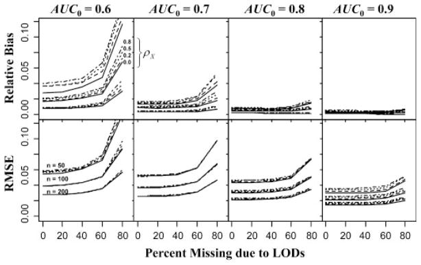
Relative bias and RMSE of maximum likelihood estimates of various levels of AUC₀ based on simulated bivariate normally distributed data of various sample sizes and correlations as a function of the percent of the non-diseased population missing due to LODs. Measurements of diseased were also affected by the LODs but to a degree that lessens as AUC₀ increases.

The empirical estimator AŨC₀, is obviously unbiased for the discriminatory ability of the BLC of the biomarkers as measured with ties for missing values below the LOD. However, Fig. 2 displays a plotting of pairs of relative bias of AÛC₀ and AŨC₀ with regard to the underlying latent AUC₀ for the various scenarios with n_x=n_y=50. This depiction shows, relatively, how consistently AŨC₀ can estimate AUC₀ with the ${\widehat{\overrightarrow{\mathrm{\beta }}}}_0^{\mathrm{T}}$ and the current measurements. Toward this end, scenarios of relative bias of AŨC₀ close to the horizontal dashed line indicating consistent estimates range from higher levels of AUC₀, (triangles=0.8, cross=0.9) and for 0, 20 and 40% missingness and also for lower AUC₀ with 40 and 60% missingness. In the latter instance, AŨC₀ displayed better consistency for AUC₀ than AŨC₀ for these small sample sizes. Figure 2 also shows the potential bias of using AÛC₀ in lieu of AŨC₀ when measurement cannot be improved.

Figure 2.

Relative bias of maximum likelihood versus empirical estimators of AUC₀ based on the estimated BLC of simulated bivariate normally distributed data of various correlations (point size) and missingness due to LODs from samples of 50 health and 50 diseased. Squares, circles, triangles and crosses indicate estimators with true AUC₀=0.6, 0.7, 0.8 and 0.9, respectively.

The coverage probability of 95% CI’s that accompanied AÛC₀ were nominal or near nominal coverage for all AUC₀ ranging from 0.890 to 0.964, 0.913 to 0.965 and 0.933 to 0.960 for n_x= n_y=50, 100 and 200, respectively. No discernable patterns exist regarding ρ_X=0, 0.2, 0.5, 0.8 or the percent missing due to the LOD. It should be noted that unlike Reiser and Faraggi’s (1997) CI for AUC using complete data, our CI’s do not take into account the bounded nature of the AUC and coverage may be adversely affected near these bounds. However, our simulation did not reflect any difficulties for the sample sizes and levels of discrimination shown. Figure 3 displays the width of MLE and bootstrapped CI’s, open and solid points, respectively, versus their coverage probability for our smallest sample size, n_x=n_y=50. Generally, CI’s increase in width to reflect uncertainty from increasing missingness, where larger point size corresponds to a larger proportion missing. Additional plots for the larger sample sizes displaying increased coverage and tighter widths are included in the Supporting Information.

Figure 3.

Confidence interval (CI) width and coverage probability of 95% CI’s estimated via maximum likelihood (open points) or bootstrapped percentiles (solid points) that accompany ML and empirical estimates of the AUC₀, respectively. True AUC₀=0.6, 0.7, 0.8 and 0.9 are identified by squares, circles, triangles and crosses/diamonds, respectively.

5 Example

To illustrate our method, we use PCBs, environmental toxicants, as potential indicators of endometriosis (Louis et al., 2005). Endometriosis is a gynecological disease exclusive to species that menstruate such as humans and other primates, occurring predominantly in women of reproductive age. Data from experimental studies in animals and observational human studies suggest an association between dioxin and PCBs and endometriosis. In our data, PCBs 153 and 180 were measured in 28 women with and 51 women without endometriosis. The biomarkers were measured jointly and were expected to be correlated. However, the sensitivity of the measurement process differed for each biomarker with PCB 153 having an LOD of d₁₅₃=0.2, resulting in 64% of the cases and 74% of the controls having unobservable levels and PCB 180 having an LOD of d₁₈₀=0.034, resulting in no missing cases but 11% of the controls having unobservable levels (Whitcomb et al., 2005).

Analyzing the biomarkers univariately, empirical methods led to AŨC₁₅₃ = 0.564 and AŨC₁₈₀ = 0.609. As measured, PCB 180 and 153 appear to have some discriminatory ability for women with endometriosis, greater for PCB 180. To investigate what potential might lie below the LODs, we can employ parametric techniques. Univariate normal distributions were assessed on the log transformed biomarkers similar to Lyles et al. (2001) via q–q plots. Figure 4 displays q–q plots where both biomarkers fit log normal distributions well, as evidenced by diagonal points corresponding to the points above the LODs. The horizontal points are essentially quantile place holders for the observations below the LOD. Assuming that the data we don’t see follow the data we do see, univariate normal likelihoods led to the MLE’s AÛC₁₅₃ = 0.511 and AÛC₁₈₀ = 0.630 for PCB 153 and PCB 180, respectively (Perkins et al., 2007). Again, PCB 180 displays a moderate ability to differentiate but the potential of PCB 153 seems to have been diminished. The result AŨC₁₅₃>AÛC₁₅₃ is due to a large “hook” in the ROC curve (Pesce and Metz, 2007) resulting from disparate variances. This behavior is rarely reflective of actual etiology but rather is likely to be a result of highly variable parameter estimates given the small sample sizes and large amount of missings. Regardless, PCB 153 might be discarded as potentially lacking discriminatory ability for endometriosis.

Figure 4.

q–q normal plots of the log transformed biomarker levels of PCBs 153 and 180 for women with endometriosis (cases) and without (controls). Horizontal points correspond to observations censored below an LOD.

However, these two biomarkers are closely linked biologically and are suspected as being highly correlated as a result of being in a mixture of environmental exposures. Using a variety of methods, we considered the joint distribution of PCB 153 and 180 to investigate whether PCB 153 might have some potential as a contributor in a BLC. First, Eq. (3) was maximized using log transformed PCB levels, MLEs for distribution parameters were calculated as well as ${\widehat{\overrightarrow{\mathrm{\beta }}}}_0^{\mathrm{T}}=\{{\mathrm{\beta }}_{153},{\mathrm{\beta }}_{180}\}=\{-1.73,1.65\}$ via Eq. (1). Using Eq. (2), we estimated that the potential from this BLC if measurements could be improved to be AÛC₀ = 0.747 with 95% CI (0.580, 0.915). This result shows that the BLC of PCBs 153 and 180 could be far superior to either biomarker alone and is potentially a good discriminator of women with and without endometriosis if the measurement sensitivity of PCB 153 could be improved. However, the sample sizes here have led to a significant but wide CI which does not rule out AUC₀<0.630.

Table 1 compares AÛC₀ to several alternative estimators of the potential AUC₀. Naïve methods to estimate potential AUC₀ in Table 1 shows the results of using replacement values (e.g. imputing a_l=d_l/2 for values below the LODs) and standard parametric methods to obtain naïve BLC, ${\widehat{\overrightarrow{\mathrm{\beta }}}}_{0R}^{\mathrm{T}}$. Imputing values in this fashion clearly violates the assumption of bivariate normality. However, we generated such estimates for the sake of comparison since standard methodology is often applied to data sets with imputed values. While these results are a slight improvement over the univariate biomarkers, it is vastly less than the proposed AÛC₀. These naïve cases also point to widely varying linear combinations, as in column 3 of Table 1.

Table 1.

Estimates of linear combinations of log PCBs 153 and 180 measured with LODs intending to maximize the AUC₀ for women with and without endometriosis using various methods.

Type of AUC0	Estimation methoda)	Estimates
		(β153, β180)	AUC0
Potential	mle	(−1.733, 1.651)	0.747
	naïve mle (d)	(0.927, 0.204)	0.639
	naïve mle (d/2)	(0.014, 0.390)	0.639
	naïve mle (E[x|x<d])	(0.138, 0.346)	0.629
As measured	mle/emp (d)	(−1.733, 1.651)	0.557
	mle/emp (d/2)	(−1.733, 1.651)	0.534
	mle/emp (E[x|x<d])	(−1.733, 1.651)	0.532
	logistic/emp (d)	(−0.322, 0.472)	0.581
	logistic/emp (d/2)	(−0.348, 0.557)	0.553
	logistic/emp (E[x|x<d])	(−0.195, 0.449)	0.575
	naïve mle/emp (d)	(0.927, 0.204)	0.608
	naïve mle/emp (d/2)	(0.014, 0.390)	0.607

The AUC₀ estimated are for the biomarker as measured with missing values below the LODs and for the potential of the latent biomarkers if they could be measured completely.

^a)Method for estimating (β₁₅₃, β₁₈₀)/method for estimating AUC₀ (replacement value used).

The second set of estimates in Table 1 begins with this BLC’s current diagnostic ability, where AŨC₀ was estimated empirically using various replacement values (d, d/2 and a_l=E[X_l|X_l<d_l], the expected values below the LODs) and the mles ${\widehat{\overrightarrow{\mathrm{\beta }}}}_0^{\mathrm{T}}$ estimated previously. These estimates vary but all are less than AŨC₁₈₀ and even AŨC₁₅₃. Alternatively, we could use these replacement values in conjunction with simple logistic regression as a means to identify the “best” coefficients to estimate AŨC₀ as measured. Lynn (2001) showed that in some cases these naïve methods can provide logistic regression coefficient estimates comparable to those using a full maximum likelihood approach for logistic regression accounting for an LOD. These “logistic” AŨC₀ in Table 1 are on par with those using the ${\widehat{\overrightarrow{\mathrm{\beta }}}}_0^{\mathrm{T}}$, “mle,” likely due to the logistic coefficients having the same signs and not grossly different proportionality. However, they do shift some of the focus to PCB 180 as evidenced by the slightly larger proportion of the linear combination, making the subsequent AŨC₀ better than AŨC₁₅₃. The ordering AŨC₁₅₃<AŨC₀<AŨC₁₈₀ is due to the difference in signs for the coefficients and in percent below the LOD for the two biomarkers. If both coefficients were positive, the order of PCB 180 would be preserved when ties from PCB 153 are introduced to a BLC and thus AŨC₀ ≥ AŨC₁₈₀. As measured, the BLC of PCBs 153 and 180 would not be of use beyond what PCB 180 can already achieve, however, Fig. 2 shows us that we need only to reduce the missingness in PCB 153 to between 20 and 40% to realize most of the difference between the potential latent and as measured effectiveness.

6 Discussion

While multiple biomarkers are often available or obtainable for the same outcome, investigators often ignore all but one and in doing so essentially throw out potential ability to discriminate beyond the biomarker they have chosen. For this reason and where biomarkers can be assumed to be normally distributed, the proposed BLC should be used in lieu of a single marker, especially in cases where multiple biomarkers come at no additional cost, as is the case with multiplex assays.

Using two biomarkers measured with LODs can result in one or both measured with censored values for an individual. The methods developed here allow us to properly account for the missing values while simultaneously taking advantage of the benefits in discriminatory ability realized by a BLC. While replacement has been shown previously to be useful in certain situations as an ad hoc approach for the AUC in the univariate case, we’ve shown here that standard parametric methods with replacement values can yield estimates of the potential AUC₀ that vary greatly from the MLE (Perkins et al., 2007). For this reason, replacing missing values by a constant is not recommended when estimating, even naïvely, the potential of a BLC of biomarkers.

The method proposed here is related to the approaches for handling censored covariates in logistic regression setting. Lynn (2001) discusses an approach for estimating the linear combination of subject-to-LOD covariates for prediction of a binary outcome. Due to the invariance of the ROC curve with respect to order-preserving transformations and because of the assumed multivariate normality of the covariates, the potential AUC₀ for Lynn’s linear combination can be computed using the standard formulation for binormal AUC. The novelty of the approach developed here is that the proposed BLC targets maximization of the AUC₀ rather than maximization of the likelihood under the logistic regression model. Depending on the parameters of the distributions the results can be either similar or substantially different (Pepe et al., 2006).

While the likelihood ratio has been demonstrated to achieve the highest possible AUC for a given set of biomarkers, in the case of two bivariate normally distributed biomarkers the absolute difference in estimated AUC can be minimal. However, this is not always the case as likelihood ratio ROC curves are assuredly “proper” or completely concave while conventional “binormal” ROC curves and those based on linear combinations of normal biomarkers can have minimal to severe non-concave portions or “hooks” (e.g. ${\mathrm{\sigma }}_X^2\gg {\mathrm{\sigma }}_Y^2$, (β⃗^TΣ_Xβ⃗)≫(β⃗^TΣ_Yβ⃗) or b≪1 from Pesce and Metz (2007)). The linear combination here has the benefit of being simple to interpret and can incorporate the empirical estimate of the biomarkers’ effectiveness as currently measured where the likelihood ratio does not. More importantly though is that in the context of the latent discriminatory ability, both would work similarly in identifying biomarkers with potential that could be measured more precisely and more extensively in the future. While, Section 3 considers the asymptotic properties of AÛC₀ for the BLC of two multivariate normal biomarkers, Section 4 shows small sample performance that is nearly unbiased and achieves nominal coverage probability for sample sizes as little as 100 with 20, 40 and 60% missing values due to LODs. The need for further investigation regarding magnitude and potential causes of differences between the likelihood- ratio and conventional “binormal” ROC curves in the context here remains.

As with all parametric estimation, this BLC of two biomarkers corrected for LODs is dependent on distributional assumptions specifically that the biomarkers or their transforms are multivariate normally distributed. The literature (Molodianovitch et al., 2006; Perkins et al., 2007) has shown MLEs of AÛC for the univariate case are robust to minor deviations from the normal assumption and unfavorable results when assumptions are grossly violated. Estimates of the AUC based on replicates of a single biomarker, a special case of the multivariate normal developments here, have shown favorable robustness by generating biomarker levels from gamma distributions (Perkins et al., 2009). While the bias was on average less than one percent of the AUC being estimated, caution and diligence should still be taken when employing this BLC resulting in AÛC₀.

A biomarker may provide differential discrimination based on some associated factor. The inclusion of this covariate information can of course be incorporated by conducting a stratified analysis for each level of such a factor. A better approach might be to directly include the covariate information in the likelihood function.

In our example we applied several methods to empirically estimate the as measured discriminatory ability, AŨC₀, by using simple replacement values in standard logistic regression or with ${\widehat{\overrightarrow{\mathrm{\beta }}}}_0^{\mathrm{T}}$. Lynn (2001) showed that in some cases, naïve replacement could yield similar logistic regression coefficient estimates to those estimated using maximum likelihood accounting for the LOD properly. We found a similar concordance here in AŨC₀ by virtue of the naïve logistic coefficients and our ${\widehat{\overrightarrow{\mathrm{\beta }}}}_0^{\mathrm{T}}$ yielded similarly proportional estimated coefficients. However, instances where this is not the case surely exist and care should be taken to investigate potential discordance before applying either BLC in practice.

These methods for estimating AUC₀ while properly accounting for missing data censored below LODs will provide an asymptotically unbiased view of the potential discriminatory ability of the BLC of a set of two biomarkers. We must note again that the AÛC₀ in this scenario reflect potential discriminatory ability and cannot be realized in practice until observations can be measured and thus allow for differentiation below the LODs. This is often the case where a less sensitive, but cheaper assay could be conducted to narrow down potential biomarkers before conducting more expensive but more precisely measured assays. We have also demonstrated the usefulness of the empirical estimate of what is possible “as measured” and how the majority of two biomarkers’ latent discriminatory ability might be realized by improving measurement, reducing missingness to between 20 and 40% rather than to zero. Estimating this potential is increasingly important as it allows researchers to focus limited resources to improve the measurement process in biomarkers that display promise and subsequently lead to improved diagnostic care.

References

- Haas CH, Scheff PA. Estimation of averages in truncated samples. Environmental Science & Technology. 1990;24:912–919. [Google Scholar]
- Hornung RW, Reed LD. Estimation of average concentration in the presence of nondetectable values. Applied Occupational and Environmental Hygiene. 1990;5:46–51. [Google Scholar]
- Louis GM, Weiner JM, Whitcomb BW, Sperrazza R, Schisterman EF, Lobdell DT, Crickard K, Greizerstein H, Kostyniak PJ. Environmental PCB exposure and risk of endometriosis. Human Reproduction. 2005;20:279–285. doi: 10.1093/humrep/deh575. [DOI] [PubMed] [Google Scholar]
- Lyles RH, Williams JK, Chuachoowong R. Correlating two viral load assays with known detection limits. Biometrics. 2001;57:1238–1244. doi: 10.1111/j.0006-341x.2001.01238.x. [DOI] [PubMed] [Google Scholar]
- Lynn HS. Maximum likelihood inference for left-censored HIV RNA data. Statistics in Medicine. 2001;20:33–45. doi: 10.1002/1097-0258(20010115)20:1<33::aid-sim640>3.0.co;2-o. [DOI] [PubMed] [Google Scholar]
- Molodianovitch K, Faraggi D, Reiser B. Comparing the areas under two correlated ROC curves: parametric and non-parametric approaches. Biometrical Journal. 2006;48:745–757. doi: 10.1002/bimj.200610223. [DOI] [PubMed] [Google Scholar]
- Pepe MS. The Statistical Evaluation of Medical Tests for Classification and Prediction. Oxford University Press; New York: 2003. [Google Scholar]
- Pepe MS, Cai T, Longton G. Combining predictors for classification using the area under the receiver operating characteristic curve. Biometrics. 2006;62:221–229. doi: 10.1111/j.1541-0420.2005.00420.x. [DOI] [PubMed] [Google Scholar]
- Perkins NJ, Schisterman EF, Vexler A. Receiver operating characteristic curve inference from a sample with a limit of detection. American Journal of Epidemiology. 2007;165:325–333. doi: 10.1093/aje/kwk011. [DOI] [PubMed] [Google Scholar]
- Perkins NJ, Schisterman EF, Vexler A. Generalized ROC curve inference for a biomarker subject to a limit of detection and measurement error. Statistics in Medicine. 2009;28:1841–1860. doi: 10.1002/sim.3575. [DOI] [PMC free article] [PubMed] [Google Scholar]
- Pesce LL, Metz CE. Reliable and computationally efficient maximum-likelihood estimation of “proper” binormal ROC curves. Academic Radiology. 2007;14:814–829. doi: 10.1016/j.acra.2007.03.012. [DOI] [PMC free article] [PubMed] [Google Scholar]
- Reiser B, Faraggi D. Confidence intervals for the generalized ROC criterion. Biometrics. 1997;53:644–652. [PubMed] [Google Scholar]
- Singh A, Nocerino J. Robust estimation of mean and variance using environmental data sets with below detection limit observations. Chemometrics and Intelligent Laboratory Systems. 2002;60:69–86. [Google Scholar]
- Su JQ, Liu JS. Linear combinations of multiple diagnostic markers. Journal of the American Statistical Association. 1993;88:1350–1355. [Google Scholar]
- Whitcomb BW, Schisterman EF, Buck GM, Weiner JM, Greizerstein H, Kostyniak PJ. Relative concentrations of organochlorines in adipose tissue and serum among reproductive age women. Environmental Toxicology and Pharmacology. 2005;19:203–213. doi: 10.1016/j.etap.2004.04.009. [DOI] [PubMed] [Google Scholar]
- Zhou XH, Obuchowski NA, McClish DK. Statistical Methods in Diagnostic Medicine. Wiley; New York: 2002. [Google Scholar]