The Generalized Hill Model: A Kinematic Approach Towards Active Muscle Contraction

Abstract

Excitation-contraction coupling is the physiological process of converting an electrical stimulus into a mechanical response. In muscle, the electrical stimulus is an action potential and the mechanical response is active contraction. The classical Hill model characterizes muscle contraction though one contractile element, activated by electrical excitation, and two non-linear springs, one in series and one in parallel. This rheology translates into an additive decomposition of the total stress into a passive and an active part. Here we supplement this additive decomposition of the stress by a multiplicative decomposition of the deformation gradient into a passive and an active part. We generalize the one-dimensional Hill model to the three-dimensional setting and constitutively define the passive stress as a function of the total deformation gradient and the active stress as a function of both the total deformation gradient and its active part. We show that this novel approach combines the features of both the classical stress-based Hill model and the recent active-strain models. While the notion of active stress is rather phenomenological in nature, active strain is micro-structurally motivated, physically measurable, and straightforward to calibrate. We demonstrate that our model is capable of simulating excitation-contraction coupling in cardiac muscle with its characteristic features of wall thickening, apical lift, and ventricular torsion.

1. Introduction

Biologically electro-active materials such as smooth muscle, skeletal muscle, and cardiac muscle undergo remarkable deformations in response to electric stimulation. For almost a century, the classical Hill model has served as a indispensable and valuable tool to model the electro-active response of living muscle (Hill, 1938). The classical Hill muscle model is a three-element model, which consists of one contractile element and two non-linear springs, one arranged in series and one in parallel (Hill, 1970). This rheology motivates the widely adopted additive decomposition of the total stress into a passive part and an active part (Nash and Panfilov, 2004). In the small strain setting, this setup kinematically translates into the additive decomposition of the total strain into a passive and an active part. In its physiological environment, however, active muscle may undergo large strains, and the small strain theory might no longer be valid. To generalize the classical Hill model to large strains setting, we multiplicatively decompose of the total deformation gradient into a passive and an active part. In contrast to previous models, which are based exclusively on a multiplicative decomposition of the deformation gradient (Ambrosi and Pezzuto, 2011), here we simultaneously adopt both, the additive decomposition of the total stress and the multiplicative decomposition of the total deformation gradient (Göktepe et al., 2013). The resulting rheology is similar to finite viscoelasticity where the active element takes the interpretation of a viscous damper (Sidoroff, 1974). In this sense, our model can be understood as the classical three-element Hill model generalized to finite deformations. As such, it is applicable to smooth, skeletal, and cardiac muscle not only in the small, but also in the large strain regime.

The modeling of cardiac tissue, however, involves several challenges that are far from being resolved thoroughly. First, the heart function is governed by electrical and mechanical activities occurring at different scales and in parallel. Furthermore, these mechanisms mutually affect one another. Therefore, the strongly coupled electromechanical cardiac response necessitates sound constitutive models and robust numerical techniques. As it is explained below, cardiac tissue has an inherently anisotropic micro-structure, which is vital for making the heart a three-dimensional biological pump. Moreover, cardiac tissue is a nonlinear material that undergoes large deformations. Hence, the developed heart models must take the geometrical and material nonlinearities into account. Apart from these, the inner surface of the ventricles is subject to transient stress traction due to the force exerted by blood during the course of every heart beat.

Undoubtedly, the highly organized and anisotropic architecture of the heart has evolved to convert the one-dimensional contraction of cardiac muscle cells, cardiac myocytes, into the three-dimensional vital pumping function of the heart. Within the cardiac micro-structure, myocytes are organized in bundles of myofibers that orderly wind around the heart, see Nielsen et al. (1991); Pope et al. (2008); Rohmer et al. (2007). The myofibers’ orientation in the ventricular walls changes from a right-handed spiral-like arrangement in the endocardium (inner wall) to a left-handed spiral-like arrangement along the epicardium (outer wall) in the transmural direction fairly smoothly. Myocytes constitute about 75% of the solid volume of the heart. Myocytes are of cylindrical shape, with a diameter of 10–25 μm and a length of up to 100 μm. On the lower scale, the myocyte cytoskeleton contains bundles of contractile myofibrils whose basic contractile unit, sarcomere, is about 2μm long. The two major protein molecules of sarcomeres are the thick myosin filaments and the thin actin filaments that slide over each other, thereby pulling the two ends (Z-lines) of the sarcomere closer together, as depicted in Figure 1. During this complex process, called cross-bridging, the myosin heads interact with the binding side of the actin filaments. Cross-bridging is initiated by calcium influx upon rapid depolarization of the myocyte from the polarized resting state with a transmembrane potential of Φ ≈ −80 mV to the depolarized state with Φ ≈ +20 mV, Bers (2002). From the depolarized state, the myocyte repolarizes back to its resting state through complex inward and outward ion dynamics across the cell membrane. Depolarization, also referred to as excitation, and repolarization result in action potentials, (Klabunde, 2005; Opie, 2004; Levy et al., 2006; Katz, 2011). Besides their remarkable contraction in response to electrical stimulation, myocytes are also capable of generating an electrical activity when subjected to mechanical loading, see Kohl et al. (1999).

Figure 1.

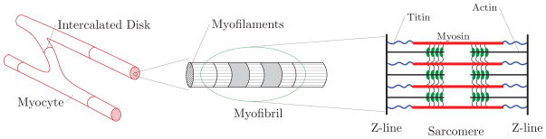
Hierarchical micro-structure of the cardiac myocyte. Cardiac myocytes exist in a striated and branched form and are connected one another through the intercalated disks. Within the organized micro-structure of cardiac myocyte, the cytoskeleton of myocytes contains bundles of contractile myofibrils, which are comprised of the basic contractile unit, sarcomere.

In the literature, the constitutive approaches to the electro-mechanically coupled response of the heart can be classified into two main groups: the active-stress models and the active-strain models. In the active-stress based models, the total stress tensor is additively decomposed into the passive and active parts. While the passive part of the stress tensor is modeled as a function of deformation only, a transmembrane potential-dependent evolution equation is used to model the active part of the stress tensor, see Nash and Panfilov (2004); Panfilov et al. (2005); Nickerson et al. (2006); Keldermann et al. (2007); Niederer and Smith (2008); Göktepe and Kuhl (2010); Lafortune et al. (2012); Eriksson et al. (2013a,b). The active-strain-based approaches can be traced back to the works by Nardinocchi and Teresi (2007); Cherubini et al. (2008) where the deformation gradient is multiplicatively decomposed into the active and elastic parts. The stress tensor is then obtained from an energy storage function, which depends only upon the elastic part of the deformation gradient. This approach has then been extended by Ambrosi et al. (2011), Nobile et al. (2012), Rossi et al. (2012) toward anisotropic constitutive models for cardiac tissue and by Stålhand et al. (2011) to model smooth muscle contraction. The active-stress and active-strain models have different pros and cons one over another from different viewpoints. As mentioned above, the active-stress approaches model the overall stress response in an additively decoupled way as in many viscoelastic material models where the equilibrium stress response and the viscous overstress response are split additively. This decomposition can be advantageous when the associated material parameters are identified by using different sets of experimental data acquired in the absence of electrical stimulation (passive) and during the active contraction, where the active and passive mechanisms co-exist. That is, the material parameters of the passive part can be obtained from the experiments where there is no electrical excitation and the material parameters of the active part can be identified from the electromechanical experiments with the parameters of the passive part frozen. From the experimental point of view, however, the direct measurement of strains is easier than the indirect measurement of the local stress fields. Furthermore, the tools of mathematical analysis is more readily available to judge the stability of a material model when the stress tensor is obtained from an energy storage function as it is the case in the active-strain models.

For almost a century, the classical Hill model (Hill, 1938) has served to model excitation-contraction coupling through a three-element rheology, where a contractile element, activated by electrical excitation, is coupled to two non-linear springs, one in series and one in parallel, see Figure 2. In the present work, we generalize the one-dimensional Hill model to the three-dimensional setting and constitutively define the passive stress as a function of the total deformation gradient and the active stress as a function of both the total deformation gradient and its active part. Therefore, the advantageous features of the both approaches are incorporated within a unified constitutive framework. To this end, inspired by the active-strain models, we decompose the total deformation gradient into the active and passive parts. The active part of the deformation gradient is considered to be dependent upon the intracellular calcium concentration whose evolution is considered to be driven by the transmembrane potential. Furthermore, the inherently anisotropic, active micro-structure of cardiac tissue is accounted for in the tensorial representation of the active part of the deformation gradient. As opposed to the above-mentioned active-strain models, where merely the active-passive split of the deformation gradient has been utilized, we further additively decompose the free energy function into passive and active parts. This decomposition allows us to recover the additively split stress structure of the active-stress models. Therefore, the proposed formulation can be considered as the generalization of the approaches that employ either additive stress decomposition or multiplicative split of the deformation gradient to account for excitation-induced contraction. This kinematic setting is embedded in a recently proposed, fully implicit, entirely finite-element-based coupled framework (Göktepe and Kuhl, 2010). The performance of the proposed formulation is demonstrated through the fully coupled finite element analysis of the non-linear excitation-contraction of a generic heart model.

Figure 2.

Schematic illustration of the generalized Hill model that consists of a passive element in the upper branch with the free energy function ψ̂^p(λ) connected to the lower active branch in parallel. The lower branch is composed of an active element characterized by the free energy function ψ̂^a(λ, λ^a) = ψ̃^a(λ^e) and an contractile element that generates active contraction λ^a upon its excitation through the action potential ϕ. The total stretch λ = λ^eλ^a is multiplicatively split into the elastic stretch λ^e and the active stretch λ^a at large strains.

The manuscript is organized as follows. In Section 2, we present the essence of the proposed novel kinematic and energetic approach to cardiac electromechanics in the one-dimensional setting where the additional complexity stemming from tensorial quantities is suppressed. For this purpose, we employ the Hill model and solve the coupled cardiac electromechanics problem locally to present the evolution of the stress response under isotonic and isometric conditions. Moreover, the sensitivity of the calcium and the active stretch transients with respect to the governing material parameters is illustrated. Section 3 is devoted to the continuous formulation of the three-dimensional the coupled electromechanics of the heart. In Section 4, the finite element formulation of the couple problem along with the consistent linerization of the residual equations is presented in the Eulerian setting. Section 5 is concerned with the specific forms of the constitutive equations and their linearization. In Section 6, the fully coupled three-dimensional finite element analysis of the non-linear excitation-contraction of a generic heart model is presented. Finally, Section 7 concludes with a critical discussion of the proposed approach.

2. Motivation: Multiplicative Active-Passive Kinematics in the One-Dimensional Setting

In this section, we motivate our micromechanically based kinematic and energetic approach within the one-dimensional framework. In the three-dimensional setting, the proposed formulation is based on the multiplicative decomposition of the deformation gradient into the active and passive parts as we set out in Section 3 in detail. In the one-dimensional setting, we decompose the total stretch λ into the passive stretch λ^e and the active stretch λ^a; that is,

$$\lambda ={\lambda }^{\mathrm{e}}{\lambda }^{\mathrm{a}},$$ (1)

where the active stretch λ^a = λ̂^a(c̄) evolves with the intracellular calcium concentration c̄. The evolution of the intracellular calcium concentration is induced by the transmembrane potential Φ and controls the underlying actively contracting cardiac tissue as schematically depicted by the contractile element in Figure 2. Alternatively, the active stretch can also be expressed as λ^a = λ̃^a(ϕ), a function of the normalized transmembrane potential ϕ, which is none other than the normalized difference between the intracellular potential and the extracellular potential.

To model the stress response of cardiac tissue, we draw from the pioneering Hill model (Hill, 1938). As schematically depicted in Figure 2, the element consists of two branches: the passive upper branch and the active lower branch, connected in parallel. In the upper branch, the response of the passive element is governed by the free energy function ψ̂^p(λ). In the lower branch, an active element and a contractile element are joined in series. While the latter generates the active contraction λ^a upon its excitation by the action potential ϕ, the response of the active element is characterized by the free energy function ψ̂^a(λ, λ^a) = ψ̃^a(λ^e). This structure results in the additive decomposition of the stress-producing energy where the total free energy ψ is split into the passive part ψ^p and the active part ψ^a

$$\psi ={\widehat{\psi }}^{\mathrm{p}}(\lambda )+{\widehat{\psi }}^{\mathrm{a}}(\lambda ,{\lambda }^{\mathrm{a}}).$$ (2)

Here, the former depends solely on the total stretch, while the latter depends on the elastic stretch, and is thus a function of both the deformation and the potential. It is worth noting that the additive structure of the free energy function (2) can be formally further extended to the form $\psi ={\widehat{\psi }}^{\mathrm{p}}(\lambda )+{\sum }_{\alpha }{\widehat{\psi }}_{\alpha }^{\mathrm{a}}(\lambda ,{\lambda }_{\alpha }^{\mathrm{a}})$ to incorporate a spectrum of active contributions. The active part of the free energy may be considered as additional energy put into muscle through electrical activation of the contractile units. Referring to the rheological representation of the generalized Hill Model in Figure 2, excitation of the active element results in contraction in this element with λ^a < 1 as depicted in Figure 5. The reduction in λ^a magnifies the stretch λ^e in the active force-generating spring in the lower branch through λ^e = λ/λ^a. This leads to additional active stress generation in the overall generalized Hill model. The additive decomposition of the free energy (2) naturally leads to the decoupled nominal stress response

Figure 5.

Sensitivity of the active stretch λ^a with respect to the material parameters ${\lambda }_{max}^{\mathrm{a}}$ and β, appear in (7). For q = 0.1, q/k = 1, and β = 3, the evolution of the active stretch λ^a for different values of ${\lambda }_{max}^{\mathrm{a}}=0.1,0.3,0.5,0.7$, and 0.9 (left). For q = 0.1, q/k = 1, and ${\lambda }_{max}^{\mathrm{a}}=0.4$, the evolution of the active stretch λ^a for different values of β = 0.5, 1.5, 10, and 50 (right). The arrows indicate changes in λ^a as the values of the respective parameters are increased.

$$P={\widehat{P}}^{\mathrm{p}}(\lambda )+{\widehat{P}}^{\mathrm{a}}(\lambda ,{\lambda }^{\mathrm{a}})$$ (3)

in terms of the passive stress P̂^p(λ) and the active stress P̂^a(λ, λ^a) that are defined as

$${\widehat{P}}^{\mathrm{p}}(\lambda ):={\partial }_{\lambda }{\widehat{\psi }}^{\mathrm{p}}(\lambda )\text{and}{\widehat{P}}^{\mathrm{a}}(\lambda ,{\lambda }^{\mathrm{a}}):={\partial }_{{\lambda }^{\mathrm{e}}}{\stackrel{\sim }{\psi }}^{\mathrm{a}}({\lambda }^{\mathrm{e}})/{\lambda }^{\mathrm{a}},$$ (4)

respectively. The passive stress response P^p represents the behavior of quiescent connective tissue and muscles. The active stress response P^a, however, is triggered by the active contraction of sarcomeres through the excitation-contraction of cardiac myocytes. As opposed to constitutive approaches based either on the active-passive decomposition of the stress response or on the active-passive decomposition of the deformation gradient, the proposed formulation captures the features of both models simultaneously. The constitutive modeling of electrically active cells goes back to the Nobel Prize-winning pioneering work of Hodgkin and Huxley (1952) on neural cells. Their model, which captures the electric response through four variables, was reduced by Fitzhugh (1961) and Nagumo et al. (1962) to a two-variable phenomenological model (Göktepe, 2013). This approach has then been followed by the action potential models of cardiac cells proposed by Noble (1962); Beeler and Reuter (1977); Luo and Rudy (1991). We also refer to Keener and Sneyd (1998); Sachse (2004); Pullan et al. (2005); Clayton and Panfilov (2008); Tusscher and Panfilov (2008) for excellent classification of the models of cardiac electrophysiology. To model the electrical activity of cardiac muscle cells, we adopt the Aliev-Panfilov model (Aliev and Panfilov, 1996) that also belongs to the class of two-variable phenomenological models. This class of models involves two ordinary differential equations for the rapidly evolving dimensionless transmembrane potential ∂_τϕ = î^ϕ(ϕ, r) and the slowly evolving recovery variable ∂_τr = î^r(ϕ, r). The specific form of these local ordinary differential equations for the Aliev-Panfilov model is given by

$$\begin{array}{l}{\partial }_{\tau }\varphi ={\widehat{i}}^{\varphi }(\varphi ,r)=c\varphi (\varphi -\alpha )(1-\varphi )-r\varphi ,\\ {\partial }_{\tau }r={\widehat{i}}^r(\varphi ,r)=\widehat{\epsilon }(\varphi ,r)[-r-c\varphi (\varphi -b-1)],\end{array}$$ (5)

in terms of the material parameters α, b, and c. The coefficient function ε̂(ϕ, r): = γ + μ₁r/(μ₂ + ϕ) governs the restitution characteristics of the model through the additional material parameters γ, μ₁, and μ₂, (Aliev and Panfilov, 1996; Göktepe and Kuhl, 2009).

The phase diagram in Figure 3 (left) depicts the solution trajectories of the local ordinary differential equations given in (5) corresponding to distinct initial points ϕ₀ and r₀ denoted by filled circles. The dashed nullclines, where î^ϕ = 0 or î^r = 0, guide the solution. The diagrams in Figure 3 (right) show the dimensionless potential ϕ and the recovery variable r curves plotted against the dimensionless time τ. The action potential is generated by adding external stimulation I = 30 to the right-hand side of (5)₁ from τ = 30 to τ = 30.02. The contraction of cardiac myocytes is triggered by calcium released from the sarcoplasmic reticulum into the cytosol. This release is initiated by excitation of myocytes where the transmembrane potential undergoes large excursions, see Figure 3 (right). To describe the intracellular calcium concentration transient during the course of the depolarization and repolarization phases, we adopt the evolution equation proposed by Pelce et al. (1995). To this end, let c̄: = c/c_R denote the normalized intracellular calcium concentration whose evolution is described by the following ordinary differential equation in terms of the dimensionless action potential ϕ

Figure 3.

The Aliev-Panfilov model with α = 0.01, γ = 0.002, b = 0.15, c = 8, μ₁ = 0.2, μ₂ = 0.3. The phase portrait depicts trajectories for distinct initial values ϕ₀ and r₀ (filled circles) converging to a stable equilibrium point (left). Non-oscillatory normalized time plot of the non-dimensional action potential ϕ and the recovery variable r (right).

$${\partial }_{\tau }\overline{c}=q\varphi -k\overline{c}$$ (6)

with the initial condition c̄(t₀) = c̄₀ = 0. In this constitutive equation, the parameters q and k control the steady-state value of c̄ and its rate of evolution. Specifically, for a given value of the dimensionless action potential ϕ, the steady-state normalized calcium concentration c̄_∞ is controlled by the ratio q/k. The parameter q governs the initial rate of evolution. To illustrate the sensitivity of the calcium transient c̄ to the parameters q and k, we first set q = 0.1, assign different values to the ratio q/k = 0.20, 0.25, 0.33, 0.50, 1, and integrate (6) for c̄. As depicted in Figure 4 (left), as the ratio q/k increases, the maximum value of c̄ increases, too. Since q = 0.1 is kept constant, however, the initial slope of c̄ curves remains unaltered. To demonstrate the sensitivity of the calcium transient c̄ to the parameter q, we keep the ratio q/k = 1 constant and solve (6) for c̄ by setting q = 0.01, 0.05, 0.1, 0.50, 1 different values. As shown in Figure 4 (right), the greater the parameter q gets, the steeper the initial rate of evolution becomes.

Figure 4.

Sensitivity of the normalized calcium concentration with respect to the material parameters q and k, appear in (6). For q = 0.1, the change of the calcium transient for different values of the ratio q/k = 0.20, 0.25, 0.33, 0.50, and 1 (left). For q/k = 1, the change of the calcium transient for different values of q = 0.01, 0.05, 0.1, 0.50, and 1 (right). The arrows indicate changes in c̄ as the values of the respective parameters are increased.

Following Pelce et al. (1995), the active stretch λ^a is considered to be a function of the normalized intracellular calcium concentration c̄ through the following relationship

$${\lambda }^{\mathrm{a}}=\frac{\xi }{1+f(\overline{c})(\xi -1)}{\lambda }_{max}^{\mathrm{a}},$$ (7)

where the parameter ${\lambda }_{max}^{\mathrm{a}}$ controls the maximum contraction and the functions f and ξ of the normalized calcium concentration c̄ are defined as

$$f(\overline{c}):=\frac{1}{2}+\frac{1}{\pi }arctan(\beta ln\overline{c})\text{and}\xi :=\frac{f({\overline{c}}_0)-1}{f({\overline{c}}_0)-{\lambda }_{max}^{\mathrm{a}}},$$ (8)

respectively. When c̄ = c̄₀ = 0, these functions take the values f(c̄₀) = 0 and $\xi ={\lambda }_{max}^{\mathrm{a}-1}$. Inserting these initial values into (7), we obtain λ^a|_t0 = 1. To illustrate the sensitivity of the active stretch λ^a to the parameters ${\lambda }_{max}^{\mathrm{a}}$ and β, we first set q/k = 1, q = 0.1, β = 3 and assign different values to ${\lambda }_{max}^{\mathrm{a}}=0.10,0.3,0.5,0.7,0.9$, and evaluate (7). As depicted in Figure 5 (left), as the ${\lambda }_{max}^{\mathrm{a}}$ increases, the maximum contraction decreases. When we fix q/k = 1, q = 0.1, ${\lambda }_{max}^{\mathrm{a}}=0.4$ and evaluate (7) for different values of β = 0.5, 1.5, 10, 50, however, for increasing β, the active stretch λ^a curve shifts upward, its shape alters, and the active stretch λ^a recovers faster.

Having the evolution of the active stretch described, we can now calculate the stress variations for isometric and isotonic experiments, where the former corresponds to a constant total stretch λ and the latter corresponds to a constant total stress P. We assume that the active and passive free energy functions have neo-Hookean form

$${\widehat{\psi }}^{\mathrm{p}}(\lambda )=E_{\mathrm{p}}[{\lambda }^2+{\lambda }^{-1}-3]\text{and}{\stackrel{\sim }{\psi }}^{\mathrm{a}}({\lambda }^{\mathrm{e}})=E_{\mathrm{a}}[{({\lambda }^{\mathrm{e}})}^2+{({\lambda }^{\mathrm{e}})}^{-1}-3]$$ (9)

with E_p and E_a denoting the corresponding moduli. This results in the specific stress expressions through the formulas in (4)

$$P^{\mathrm{p}}(\lambda )=E_{\mathrm{p}}[2\lambda -{\lambda }^{-2}]\text{and}{P}^{\mathrm{a}}({\lambda }^{\mathrm{e}})=E_{\mathrm{a}}[2{\lambda }^{\mathrm{e}}-{({\lambda }^{\mathrm{e}})}^{-2}]{({\lambda }^{\mathrm{a}})}^{-1}.$$ (10)

In the isometric experiment, the total stretch is fixed at λ̄ = 1.2 and the variation of the stresses is calculated during the course of action potential. As depicted in Figure 6 (left), the depolarization of the active element initiates an active stretch, see also Figure 5, which, in turn, brings about an increase in the active stress P^a with a physiological delay. Upon repolarization, the active stress relaxes back to its resting value. In the isotonic experiment, the total stress is kept constant at P = 1.15 and the stress sharing between the active and passive elements is computed. As depicted in Figure 6 (right), the excitation-induced contraction of the contractile element leads to an increase in the active stress P^a. Upon the repolarization, the active stress relaxes back to its resting value. Accordingly, the passive stress undergoes reverse changes to keep the total stress constant. The above-outlined illustrations aim to give the essence of the three-dimensional model, discussed in the upcoming sections.

Figure 6.

The evolution of the active stress P^a and the passive stress P^p under isometric (left) the isotonic (right) conditions. In the isometric experiment, the total stretch is fixed to the value λ̄ = 1.2 and the variation of the stresses is observed during the course of action potential. In the isotonic experiment, however, the total stress is kept constant at P = 1.15 and the stress sharing between the active and passive branches is monitored. The action potential is generated as described in Figure 3 with the parameters given therein. For the evolution of the calcium concentration c̄ and the active stretch λ^a, we used q = 0.1, q/k = 1, β = 3, and ${\lambda }_{max}^{\mathrm{a}}=0.4$. The values of the active and passive moduli in (10) are taken as E_p = E_a = 0.35.

3. Coupled Cardiac Electromechanics

In this section, we outline the general three-dimensional framework of the coupled electromechanics of the heart. A coupled initial boundary-value problem of cardiac electromechanics within the mono-domain setting is formulated in terms of the two primary field variables, namely the placement φ(X, t) and the transmembrane potential Φ(X, t). While the latter refers to a potential difference between the intracellular medium and the extracellular medium within the context of mono-domain formulations of cardiac electrophysiology, see Keener and Sneyd (1998), the former is the non-linear deformation map, depicted in Figure 7. Evolution of the primary field variables is governed by two basic field equations: the balance of linear momentum and the reaction-diffusion-type equation of excitation, which are introduced in Section 3.2.

Figure 7.

Motion of an excitable and deformable solid body in the Euclidean space ℝ³ through the non-linear deformation map φ_t(X) at time t. The deformation gradient F = ∇_Xφ_t(X) describes the tangent map between the respective tangent spaces. The deformation gradient F is multiplicatively decomposed into the passive part F^e and the active part F^a with denoting the fictitious, incompatible intermediate vector space.

3.1. Kinematics: Active-Passive Decomposition

Let ⊂ ℝ³ denote the reference configuration of an excitable and deformable solid body that occupies the current configuration ⊂ ℝ³ at time t ∈ ℝ₊ as shown Figure 7. Accordingly, material points X ∈ are mapped onto their spatial positions x ∈ through the non-linear deformation map x = φ_t(X): → at time t. The deformation gradient F: = ∇_Xφ_t(X): T_X → T_x acts as the tangent map between the tangent spaces of the respective configurations. The gradient operator ∇_X[•] denotes the spatial derivative with respect to the reference coordinates X and the Jacobiain J: = det F > 0 is the volume map.

Inspired by the kinematics of finite plasticity (Kröner (1960); Lee (1969)) and the recent work by Cherubini et al. (2008), the deformation gradient is multiplicatively decomposed into the passive part F^e and the active part F^a

$$\mathit{F}={\mathit{F}}^{\mathrm{e}}{\mathit{F}}^{\mathrm{a}}.$$ (11)

The multiplicative decomposition of the deformation gradient inherently results in a fictitious, incompatible intermediate vector space where, as opposed to the total deformation gradient F, neither F^e nor F^a is related to a gradient of any non-linear deformation map, see Figure 7. The active part of the deformation gradient F^a evolves with the transmembrane potential Φ and reflects the underlying actively contracting anisotropic architecture of cardiac tissue through its dependence upon the second-order structural tensors A_m, A_n, and A_k

$${\mathit{F}}^{\mathrm{a}}={\widehat{\mathit{F}}}^{\mathrm{a}}(\mathrm{\Phi },{\mathit{A}}_{\mathrm{m}},{\mathit{A}}_{\mathrm{n}},{\mathit{A}}_{\mathrm{k}}).$$ (12)

For an orthotropic contractile material, the active part of the deformation gradient can be expressed as

$${\mathit{F}}^{\mathrm{a}}=\mathbf{1}+({\lambda }_{\mathrm{m}}^{\mathrm{a}}-1){\mathit{A}}_{\mathrm{m}}+({\lambda }_{\mathrm{n}}^{\mathrm{a}}-1){\mathit{A}}_{\mathrm{n}}+({\lambda }_{\mathrm{k}}^{\mathrm{a}}-1){\mathit{A}}_{\mathrm{k}}$$ (13)

where ${\lambda }_{\alpha }^{\mathrm{a}}={\widehat{\lambda }}_{\alpha }^{\mathrm{a}}(\mathrm{\Phi })$ for α = m, k, n. The compatibility of the overall deformation is then satisfied by the passive part of the deformation gradient F^e. This is evident from the fact that while F^a is rotation-free with respect to the material directions, F^e embodies the rotational part.

3.2. Governing Field Equations: Strong Form

The balance of linear momentum with its following well-known local spatial form

$$J\text{div}[J^{-1}\widehat{\mathit{\tau }}]+\mathit{B}=\mathbf{0}\text{in}\mathcal{B}$$ (14)

describes the quasi-static stress equilibrium in terms of the Eulerian Kirchhoff stress tensor τ̂ and a given body force B per unit reference volume. The operator div[•] denotes the divergence with respect to the spatial coordinates x. Note that the momentum balance depends on both primary field variables, the deformation field and the electrical field, through the Kirchhoff stress tensor τ̂, whose particular form is elaborated in Section 5. The essential (Dirichlet) and natural (Neumann) boundary conditions, see Figure 8 (left),

Figure 8.

Illustration of the mechanical (left) and electrophysiological (right) Dirichlet (essential) and Neumann (natural) boundary conditions. For the mechanical problem, Dirichlet and Neumann boundary conditions are prescribed on the boundaries ∂ and ∂ , respectively. For the electrical problem, ∂ and ∂ denote the boundaries where the corresponding Dirichlet and Neumann boundary conditions are defined separately. These sub-boundaries are complementary ∂ = ∂ ∪ ∂ , ∂ = ∂ ∪ ∂ and disjoint ∂ ∩ ∂ = ∅, ∂ ∩ ∂ = ∅.

$$\mathit{\phi }=\overline{\mathit{\phi }}\text{on}\partial {\mathcal{S}}_{\phi }\text{and}\mathit{t}=\overline{\mathit{t}}\text{on}\partial {\mathcal{S}}_t,$$ (15)

complete the description of the mechanical problem. Clearly, the surface subdomains ∂ and ∂ fulfill the conditions ∂ = ∂ ∪ ∂ and ∂ ∩ ∂ = ∅. The surface stress traction vector t̄, defined on ∂ , is related to the Cauchy stress tensor through the Cauchy stress theorem t̄: = J⁻¹τ · n where n is the outward surface normal on ∂ .

The second field equation of the coupled problem, the excitation equation

$$\stackrel{.}{\mathrm{\Phi }}-J\text{div}[J^{-1}\widehat{\mathit{q}}]-{\widehat{I}}^{\varphi }=0\text{in}\mathcal{B}$$ (16)

describes the spatio-temporal evolution of the action potential field Φ(X, t) in terms of the diffusion term div[J⁻¹q̂] and the non-linear current term Î^ϕ. The notation [•˙]: = D[•]/Dt denotes the material time derivative. Within the framework of FitzHugh-Nagumo-type models of electrophysiology (Fitzhugh, 1961; Nagumo et al., 1962), the current source Î^ϕ controls the characteristics of the action potential regarding its shape, duration, restitution, and hyperpolarization along with another variable, the so-called recovery variable r whose evolution is governed by an additional ordinary differential equation (5)₂. Since the recovery variable r chiefly controls the local repolarization behavior of the action potential, we treat it as a local internal variable. Similar to the momentum balance (14), the excitation equation is also subject to the corresponding essential and natural boundary conditions, Fig. 8 (right),

$$\mathrm{\Phi }=\overline{\mathrm{\Phi }}\text{on}\partial {\mathcal{S}}_{\varphi }\text{and}h=\overline{h}\text{on}\partial {\mathcal{S}}_h,$$ (17)

respectively. Evidently, the surface subdomains ∂ and ∂ are disjoint, ∂ ∩ ∂ = ∅, and complementary, ∂ = ∂ ∪ ∂ . The electrical surface flux term h̄ in (17)₂ is related to the spatial flux vector q̂ through the Cauchy-type formula $\overline{h}:=J^{-1}\widehat{\mathit{q}}·\mathit{n}$ in terms of the spatial surface normal n. The transient term in the excitation equation (16) requires an initial condition for the potential field at t = t₀

$${\mathrm{\Phi }}_0(\mathit{X})=\mathrm{\Phi }(\mathit{X},t_0)\text{in}\mathcal{B}.$$ (18)

Note that the “hat” symbol used along with the terms τ̂, q̂, and Î^ϕ indicates that these variables are dependent on the primary fields.

3.3. Constitutive Equations

The solution of the field equations requires the knowledge of constitutive equations describing the Kirch-hoff stress tensor τ̂, the potential flux q̂, and the current source Î^ϕ. Similar to Section 2 and in contrast to the literature (Cherubini et al. (2008); Ambrosi et al. (2011)), we additively decompose the free energy function into the passive part Ψ^p and the active part Ψ^a as similarly established in the modeling of electroactive polymers, see e.g. Ask et al. (2012a,b),

$$\mathrm{\Psi }={\mathrm{\Psi }}^{\mathrm{p}}(\mathit{g};\mathit{F})+{\widehat{\mathrm{\Psi }}}^{\mathrm{a}}(\mathit{g};{\mathit{F}}^{\mathrm{e}})$$ (19)

where the former depends solely on the total deformation gradient, while the latter depends on the elastic part of the deformation gradient, thus both on the deformation and on the potential. This additive form results in the decoupled stress response

$$\mathit{\tau }={\widehat{\mathit{\tau }}}^{\mathrm{p}}(\mathit{g};\mathit{F})+{\widehat{\mathit{\tau }}}^{\mathrm{a}}(\mathit{g};{\mathit{F}}^{\mathrm{e}})$$ (20)

where the Kirchhoff stress tensor is obtained by the Doyle-Ericksen formula τ := 2∂_g Ψ and the elastic part of the deformation gradient is obtained as F^e = F F^a−1 from (11). Since the formulation is laid out in the Eulerian setting, the current metric g is explicitly included in the arguments of the constitutive functions. For detailed background information on the formulation of anisotropic elasticity in terms of the Eulerian quantities the reader is referred to Menzel and Steinmann (2003b), while the multiplicative decompositzion with application to anisotropic plasticity is addressed in Menzel and Steinmann (2003a) and the modeling of anisotropic growth is discussed in Menzel (2007).

The potential flux q̂ is assumed to depend linearly on the spatial potential gradient ∇_xΦ

$$\widehat{\mathit{q}}=\mathit{D}(\mathit{g};\mathit{F})·{\nabla }_x\mathrm{\Phi }$$ (21)

through the deformation-dependent anisotropic spatial conduction tensor D(g; F) that governs the conduction speed of the non-planar depolarization front in three-dimensional anisotropic cardiac tissue.

The last constitutive relation, which describes the electrical source term of the Fitzhugh-Nagumo-type excitation equation (16), is additively decomposed into the excitation-induced purely electrical part ${\widehat{I}}_{\mathrm{e}}^{\varphi }(\mathrm{\Phi },r)$ and the stretch-induced mechano-electrical part ${\widehat{I}}_{\mathrm{m}}^{\varphi }(\mathit{g};\mathit{F},\mathrm{\Phi })$; that is,

$${\widehat{I}}^{\varphi }={\widehat{I}}_{\mathrm{e}}^{\varphi }(\mathrm{\Phi },r)+{\widehat{I}}_{\mathrm{m}}^{\varphi }(\mathit{g};\mathit{F},\mathrm{\Phi }).$$ (22)

The former describes the effective current generation due to the inward and outward flow of ions across the cell membrane. This ionic flow is triggered by a perturbation of the resting potential beyond some physical threshold upon the arrival of the depolarization front. The latter, however, incorporates the opening of ion channels under the action of deformation, see Kohl et al. (1999).

Apart from the primary field variables, the recovery variable r, which describes the repolarization response of the action potential, appears among the arguments of ${\widehat{I}}_{\mathrm{e}}^{\varphi }$ in (22). The evolution of the recovery variable r chiefly determines the local shape and duration of the action potential inherent to each cardiac cell and may change throughout the heart. For this reason, evolution of the recovery variable r is commonly modeled by a local ordinary differential equation ṙ = î^r(Φ, r) as in (5)₂. From an algorithmic point of view, the local nature of this evolution equation allows us to treat the recovery variable as an internal variable. This is one of the key features of the proposed formulation that preserves the modular global structure of the field equations (Göktepe and Kuhl (2009); Göktepe et al. (2010); Göktepe and Kuhl (2010); Dal et al. (2012, 2013); Wong et al. (2011, 2013)).

4. Finite Element Formulation of the Coupled Cardiac Electromechanics

In this section, we construct the weak integral forms of the strong non-linear field equations of the coupled electromechanical problem (14,16) introduced in the preceding section and linearize them consistently in the Eulerian setting. To this end, the placement φ(X, t) and potential Φ(X, t) fields are discretized to transform the continuous integral equation for the non-linear weighted residual and for the Newton-type update into a set of coupled, discrete algebraic equations. The resulting set of algebraic equations is then solved monolithically and iteratively for the nodal degrees of freedom.

4.1. Weak formulation

To construct the weak forms of the governing field equations, we multiply the residual equations (14,16) by the square-integrable weight functions δφ ∈ and δΦ ∈ that satisfy the essential boundary conditions δφ = 0 on ∂ and δΦ = 0 on ∂ . The weighted residual equations are then integrated over the solid volume. Integrating by parts, we obtain the following weighted residual expressions for the balance of linear momentum (14)

$$G^{\phi }(\delta \mathit{\phi },\mathit{\phi },\mathrm{\Phi })=G_{int}^{\phi }(\delta \mathit{\phi },\mathit{\phi },\mathrm{\Phi })-G_{\text{ext}}^{\phi }(\delta \mathit{\phi })=0$$ (23)

and for the reaction-diffusion equation (16)

$$G^{\varphi }(\delta \mathrm{\Phi },\mathit{\phi },\mathrm{\Phi })=G_{int}^{\varphi }(\delta \mathrm{\Phi },\mathit{\phi },\mathrm{\Phi })-G_{\text{ext}}^{\varphi }(\delta \mathrm{\Phi },\mathit{\phi },\mathrm{\Phi })=0.$$ (24)

Explicit forms of the internal $G_{int}^{\phi }$ and external $G_{\text{ext}}^{\phi }$ residual terms in (23) are defined as

$$G_{int}^{\phi }(\delta \mathit{\phi },\mathit{\phi },\mathrm{\Phi }):={\int }_{\mathcal{B}}{\nabla }_x(\delta \mathit{\phi }):\widehat{\mathit{\tau }}\mathrm{d}V,G_{\text{ext}}^{\phi }(\delta \mathit{\phi }):={\int }_{\mathcal{B}}\delta \mathit{\phi }·\mathit{B}\mathrm{d}V+{\int }_{\partial {\mathcal{S}}_t}\delta \mathit{\phi }·\overline{\mathit{t}}\mathrm{d}a,$$ (25)

where the body force B and the surface traction t̄ are assumed to be given. Analogously, the following expressions for $G_{int}^{\varphi }$ and $G_{\text{ext}}^{\varphi }$ are given as

$$G_{int}^{\varphi }(\delta \mathrm{\Phi },\mathit{\phi },\mathrm{\Phi }):={\int }_{\mathcal{B}}(\delta \mathrm{\Phi }\stackrel{.}{\mathrm{\Phi }}+{\nabla }_x(\delta \mathrm{\Phi })·\widehat{\mathit{q}})\mathrm{d}V,G_{\text{ext}}^{\varphi }(\delta \mathrm{\Phi },\mathit{\phi },\varphi ):={\int }_{\mathcal{B}}\delta \mathrm{\Phi }{\widehat{I}}^{\varphi }\mathrm{d}V+{\int }_{\partial {\mathcal{S}}_h}\delta \mathrm{\Phi }\overline{h}\mathrm{d}a,$$ (26)

respectively. The surface flux h̄ is prescribed as a natural boundary condition through (17)₂. Unlike the mechanical external residual $G_{\text{ext}}^{\phi }$ in (25)₂, the electrical external residual $G_{\text{ext}}^{\varphi }$ depends explicitly upon the field variables. We discretize the time space := [0, t] into n_stp divisions such that $\mathcal{T}={\cup }_{n=0}^{n_{\text{stp}}-1}[t_n,t_{n+1}]$. We denote the time increment as Δt := t − t_n and omit the subscript “n + 1” for the sake of conciseness. We then use the implicit Euler scheme to compute the time derivative of the potential Φ at time t

$$\stackrel{.}{\mathrm{\Phi }}\approx (\mathrm{\Phi }-{\mathrm{\Phi }}_n)/\mathrm{\Delta }t$$ (27)

with Φ_n := Φ(X, t_n). Using this finite difference approximation for Φ̇ in (26)₁ we end up with the following algorithmic form

$$G_{int}^{\varphi ,\text{algo}}(\delta \mathrm{\Phi },\mathit{\phi },\mathrm{\Phi })={\int }_{\mathcal{B}}(\delta \mathrm{\Phi }\frac{\mathrm{\Phi }-{\mathrm{\Phi }}_n}{\mathrm{\Delta }t}+{\nabla }_x(\delta \mathrm{\Phi })·\widehat{\mathit{q}})\mathrm{d}V.$$ (28)

Next, we carry out the consistent linearization for the algorithmic solution.

4.2. Consistent algorithmic linearization

The geometric and material non-linearities in the weighted residual equations (23,24) arise from the spatial gradient operators and the non-linear constitutive equations introduced in Section 3.3. Since we propose to adopt a monolithic solution scheme in the proposed formulation, the simultaneous solution of these coupled equations requires utilization of Newton-type iterative methods within the context of the implicit finite element method. For this purpose, the weighted residuals (23,24) are consistently linearized with respect to the field variables about an intermediate iteration step where the field variables take the values φ̃ and Φ̃.

$$\begin{array}{l}\text{Lin}{G}^{\phi }(\delta \mathit{\phi },\mathit{\phi },\mathrm{\Phi }){\mid }_{\stackrel{\sim }{\mathit{\phi }},\stackrel{\sim }{\mathrm{\Phi }}}:=G^{\phi }(\delta \mathit{\phi },\stackrel{\sim }{\mathit{\phi }},\stackrel{\sim }{\mathrm{\Phi }})+\mathrm{\Delta }{G}^{\phi }(\delta \mathit{\phi },\stackrel{\sim }{\mathit{\phi }},\stackrel{\sim }{\mathrm{\Phi }};\mathrm{\Delta }\mathit{\phi },\mathrm{\Delta }\mathrm{\Phi })=0,\\ \text{Lin}{G}^{\varphi }(\delta \mathrm{\Phi },\mathit{\phi },\mathrm{\Phi }){\mid }_{\stackrel{\sim }{\mathit{\phi }},\stackrel{\sim }{\mathrm{\Phi }}}:=G^{\varphi }(\delta \varphi ,\stackrel{\sim }{\mathit{\phi }},\stackrel{\sim }{\mathrm{\Phi }})+\mathrm{\Delta }{G}^{\varphi }(\delta \mathrm{\Phi },\stackrel{\sim }{\mathit{\phi }},\stackrel{\sim }{\mathrm{\Phi }};\mathrm{\Delta }\mathit{\phi },\mathrm{\Delta }\mathrm{\Phi })=0.\end{array}$$ (29)

Analogous to (23,24), the incremental terms ΔG^φ and ΔG^ϕ can be expressed as

$$\mathrm{\Delta }{G}^{\phi }=\mathrm{\Delta }{G}_{int}^{\phi }-\mathrm{\Delta }{G}_{\text{ext}}^{\phi }\text{and}\mathrm{\Delta }{G}^{\varphi }=\mathrm{\Delta }{G}_{int}^{\varphi }-\mathrm{\Delta }{G}_{\text{ext}}^{\varphi }.$$ (30)

We start with deriving the increment $\mathrm{\Delta }{G}_{int}^{\phi }$ according to (25)₁

$$\mathrm{\Delta }{G}_{int}^{\phi }={\int }_{\mathcal{B}}\mathrm{\Delta }({\nabla }_x(\delta \mathit{\phi })):\widehat{\mathit{\tau }}+{\nabla }_x(\delta \mathit{\phi }):\mathrm{\Delta }\widehat{\mathit{\tau }}\mathrm{d}V.$$ (31)

Linearization of the non-linear terms in (31) yields

$$\mathrm{\Delta }({\nabla }_x(\delta \mathit{\phi }))=-{\nabla }_x(\delta \mathit{\phi }){\nabla }_x(\mathrm{\Delta }\mathit{\phi })\text{and}\mathrm{\Delta }\widehat{\mathit{\tau }}={\mathcal{L}}_{\mathrm{\Delta }\mathit{\phi }}\widehat{\mathit{\tau }}+{\nabla }_x(\mathrm{\Delta }\mathit{\phi })\widehat{\mathit{\tau }}+\widehat{\mathit{\tau }}{\nabla }_x^T(\mathrm{\Delta }\mathit{\phi })+{\mathit{C}}^{\phi \varphi }\mathrm{\Delta }\mathrm{\Phi },$$ (32)

where τ̂ denotes the objective Lie derivative along the increment Δφ. The latter can be expressed as

$${\mathcal{L}}_{\mathrm{\Delta }\mathit{\phi }}\widehat{\mathit{\tau }}={ℂ}^{\phi \phi }:\frac{1}{2}{\mathcal{L}}_{\mathrm{\Delta }\mathit{\phi }}\mathit{g}={ℂ}^{\phi \phi }:(\mathit{g}{\nabla }_x(\mathrm{\Delta }\mathit{\phi }))$$ (33)

in terms of the Lie derivative of the current metric ${\mathcal{L}}_{\mathrm{\Delta }\mathit{\phi }}\mathit{g}=\mathit{g}{\nabla }_x(\mathrm{\Delta }\mathit{\phi })+{\nabla }_x^T(\mathrm{\Delta }\mathit{\phi })\mathit{g}$. The fourth-order spatial tangent moduli in (33) and the sensitivity of the Kirchhoff stresses to the action potential C^φϕ introduced in (32)₂ are defined as

$${ℂ}^{\phi \phi }:=2{\partial }_{\mathit{g}}\widehat{\mathit{\tau }}(\mathit{g};\mathit{F},\mathrm{\Phi })\text{and}{\mathit{C}}^{\phi \varphi }:={\partial }_{\mathrm{\Phi }}\widehat{\mathit{\tau }}(\mathit{g};\mathit{F},\mathrm{\Phi }),$$ (34)

respectively. Incorporating the results (32) along with (33,34) in (31), we arrive at the following expression

$$\mathrm{\Delta }{G}_{int}^{\phi }={\int }_{\mathcal{B}}{\nabla }_x(\delta \mathit{\phi }):{ℂ}^{\phi \phi }:(\mathit{g}{\nabla }_x(\mathrm{\Delta }\mathit{\phi }))\mathrm{d}V+{\int }_{\mathcal{B}}{\nabla }_x(\delta \mathit{\phi }):({\nabla }_x(\mathrm{\Delta }\mathit{\phi })\widehat{\mathit{\tau }})\mathrm{d}V+{\int }_{\mathcal{B}}{\nabla }_x(\delta \mathit{\phi }):{\mathit{C}}^{\phi \varphi }{\mathrm{\Delta }}^{\mathrm{\Phi }}\mathrm{d}V,$$ (35)

where the three integral terms on the right-hand side illustrate the existing nonlinearities arising from the entirely mechanical material response, from the geometry, and from the coupled electromechanical stress response, respectively. Because the body force B and the traction boundary conditions t̄ in (25)₂ are given and assumed to represent dead loads, the external mechanical term vanishes identically $\mathrm{\Delta }{G}_{\text{ext}}^{\phi }=0$ such that $\mathrm{\Delta }{G}^{\phi }\equiv \mathrm{\Delta }{G}_{int}^{\phi }$.

By using the explicit algorithmic form of $G_{int}^{\varphi }$ in (28), the increment $\mathrm{\Delta }{G}_{int}^{\varphi }$ can be expressed as

$$\mathrm{\Delta }{G}_{int}^{\varphi }={\int }_{\mathcal{B}}\delta \mathrm{\Phi }\frac{\mathrm{\Delta }\mathrm{\Phi }}{\mathrm{\Delta }t}+\mathrm{\Delta }({\nabla }_x\delta \mathrm{\Phi })·\widehat{\mathit{q}}+{\nabla }_x(\delta \mathrm{\Phi })·\mathrm{\Delta }\widehat{\mathit{q}}\mathrm{d}V.$$ (36)

Akin to (32)₁, the linearization of ∇_x(δΦ) becomes Δ(∇_x(δΦ)) = −∇_x(δΦ) ∇_x(Δφ). Based on the functional definition of the spatial potential flux q̂ in (21), we obtain

$$\mathrm{\Delta }\widehat{\mathit{q}}={\mathcal{L}}_{\mathrm{\Delta }\mathit{\phi }}\widehat{\mathit{q}}+{\nabla }_x(\mathrm{\Delta }\mathit{\phi })·\widehat{\mathit{q}}+\widehat{\mathit{D}}·{\nabla }_x(\mathrm{\Delta }\mathrm{\Phi })$$ (37)

where q̂ denotes the incremental Lie derivative of the potential flux q̂ and is defined as

$${\mathcal{L}}_{\mathrm{\Delta }\mathit{\phi }}\widehat{\mathit{q}}={\mathcal{C}}^{\varphi \phi }:\frac{1}{2}{\mathcal{L}}_{\mathrm{\Delta }\mathit{\phi }}\mathit{g}={\mathcal{C}}^{\varphi \phi }:(\mathit{g}{\nabla }_x(\mathrm{\Delta }\mathit{\phi })).$$ (38)

The second-order deformation-dependent conduction tensor D̂ and the third-order mixed moduli , introduced in (37,38), are defined as

$$\widehat{\mathit{D}}:={\partial }_{{\nabla }_x\mathrm{\Phi }}\widehat{\mathit{q}}(\mathit{g};\mathit{F},\mathrm{\Phi })\text{and}{\widehat{\mathcal{C}}}^{\varphi \phi }:=2{\partial }_{\mathit{g}}\widehat{\mathit{q}}(\mathit{g};\mathit{F},\mathrm{\Phi }).$$ (39)

Making use of the result (37) and the definitions (38,39) in (36), we obtain

$$\mathrm{\Delta }{G}_{int}^{\varphi }={\int }_{\mathcal{B}}\delta \mathrm{\Phi }\frac{\mathrm{\Delta }\mathrm{\Phi }}{\mathrm{\Delta }t}\mathrm{d}V+{\int }_{\mathcal{B}}{\nabla }_x(\delta \mathrm{\Phi })·\widehat{\mathit{D}}·{\nabla }_x(\mathrm{\Delta }\mathrm{\Phi })\mathrm{d}V+{\int }_{\mathcal{B}}{\nabla }_x(\delta \mathrm{\Phi })·{\mathcal{C}}^{\varphi \phi }:(\mathit{g}{\nabla }_x(\mathrm{\Delta }\mathit{\phi }))\mathrm{d}V.$$ (40)

Observe that as opposed to $G_{\text{ext}}^{\phi }$, the external term $G_{\text{ext}}^{\varphi }$ in (24) depends non-linearly on the field variables through the source term Î^ϕ(g; F, Φ) introduced in (22). For a given h̄ on ∂ , the following expression is obtained for the incremental external electrical residual

$$\mathrm{\Delta }{G}_{\text{ext}}^{\varphi }:={\int }_{\mathcal{B}}\delta \mathrm{\Phi }\mathrm{\Delta }{\widehat{I}}^{\varphi }\mathrm{d}V.$$ (41)

In the Eulerian setting, the linearization of the function Î^ϕ yields

$$\mathrm{\Delta }{\widehat{I}}^{\varphi }=\mathit{H}:(\mathit{g}{\nabla }_x(\mathrm{\Delta }\mathit{\phi }))+H\mathrm{\Delta }\mathrm{\Phi }$$ (42)

where the tangents H and H are defined as

$$\mathit{H}:=2{\partial }_{\mathit{g}}{\widehat{I}}^{\varphi }(\mathit{g};\mathit{F},\mathrm{\Phi })\text{and}H:={\partial }_{\mathrm{\Phi }}{\widehat{I}}^{\varphi }(\mathit{g};\mathit{F},\mathrm{\Phi }),$$ (43)

respectively. Recalling the additive split introduced in (22), the scalar tangent term H can be expressed as

$$H=H_{\mathrm{e}}+H_{\mathrm{m}}\text{with}{H}_{\mathrm{e}}:={\partial }_{\mathrm{\Phi }}{\widehat{I}}_{\mathrm{e}}^{\varphi }\text{and}{H}_{\mathrm{m}}:={\partial }_{\mathrm{\Phi }}{\widehat{I}}_{\mathrm{m}}^{\varphi }.$$ (44)

Substituting the results (42,43) into (41), we obtain the external electrical increment

$$\mathrm{\Delta }{G}_{\text{ext}}^{\varphi }={\int }_{\mathcal{B}}\delta \mathrm{\Phi }(\mathit{H}:(\mathit{g}{\nabla }_x(\mathrm{\Delta }\mathit{\phi }))+H\mathrm{\Delta }\mathrm{\Phi })\mathrm{d}V.$$ (45)

The last expression concludes the consistent linearization of the residual integrals within the continuous spatial setting. In what follows, we discretize the governing equations in space to obtain the discrete algebraic counterparts of the residual expressions (25,26).

4.3. Spatial discretization

By following the conventional isoparametric Galerkin procedure, we approximate the continuous integral equations of the weak forms (23,24). For this purpose, we discretize the domain of interest into element subdomains ${\mathcal{B}}_e^h$ such that $\mathcal{B}\approx {\mathcal{B}}^h={\cup }_{e=1}^{n_{\mathrm{e}1}}{\mathcal{B}}_e^h$ where n_el is the total number of elements. The primary fields and the associated weight functions are interpolated over each element domain through the corresponding discrete nodal values and shape functions

$$\begin{array}{ccc}\delta {\mathit{\phi }}_e^h=\sum _{i=1}^{n_{\text{en}}}{N}^i\delta {\mathit{x}}_i^e& \text{and}& \delta {\mathrm{\Phi }}_e^h=\sum _{k=1}^{n_{\text{en}}}{N}^k\delta {\mathrm{\Phi }}_k^e,\\ {\mathit{\phi }}_e^h=\sum _{j=1}^{n_{\text{en}}}{N}^j{\mathit{x}}_j^e& \text{and}& {\mathrm{\Phi }}_e^h=\sum _{l=1}^{n_{\text{en}}}{N}^l{\mathrm{\Phi }}_l^e,\end{array}$$ (46)

where n_en refers to the number of nodes per element. Based on the discretization (46), the spatial gradients of the weight functions are obtained as

$${\nabla }_x(\delta {\mathit{\phi }}_e^h)=\sum _{i=1}^{n_{\text{en}}}\delta {\mathit{x}}_i^e\otimes {\nabla }_x{N}^i\text{and}{\nabla }_x(\delta {\mathrm{\Phi }}_e^h)=\sum _{k=1}^{n_{\text{en}}}\delta {\varphi }_k^e{\nabla }_x{N}^k.$$ (47)

Analogously, the spatial gradients of the incremental fields become

$${\nabla }_x(\mathrm{\Delta }{\mathit{\phi }}_e^h)=\sum _{j=1}^{n_{\text{en}}}\mathrm{\Delta }{\mathit{x}}_j^e\otimes {\nabla }_x{N}^j\text{and}{\nabla }_x(\mathrm{\Delta }{\mathrm{\Phi }}_e^h)=\sum _{l=1}^{n_{\text{en}}}\mathrm{\Delta }{\mathrm{\Phi }}_l^e{\nabla }_x{N}^l.$$ (48)

Inserting the discretized representations (46,47) into (23,24), we end up with the discrete residual vectors

$$\begin{array}{l}{\mathit{R}}_I^{\phi }={\mathrm{A}}_{e=1}^{n_{\text{el}}}\{{\int }_{{\mathcal{B}}_e^h}{\nabla }_x{N}^i·\widehat{\mathit{\tau }}\mathrm{d}V-{\int }_{{\mathcal{B}}_e^h}{N}^i\mathit{B}\mathrm{d}V-{\int }_{\partial {\mathcal{S}}_t^e}{N}^i\overline{\mathit{t}}\mathrm{d}a\}=0,\\ R_J^{\varphi }={\mathrm{A}}_{e=1}^{n_{\text{el}}}\{{\int }_{{\mathcal{B}}_e^h}(N^j\frac{\mathrm{\Phi }-{\mathrm{\Phi }}_n}{\mathrm{\Delta }t}+{\nabla }_x{N}^j·\widehat{\mathit{q}})\mathrm{d}V-{\int }_{{\mathcal{B}}_e^h}{N}^j{\widehat{I}}^{\varphi }\mathrm{d}V-{\int }_{\partial {\mathcal{S}}_h^e}{N}^j\overline{h}\mathrm{d}a\}=0.\end{array}$$ (49)

Likewise, substituting the discretizations (46,47,48) into (31,40,45), we obtain the discrete tangent matrices

$$\begin{array}{l}{\mathit{K}}_{IJ}^{\phi \phi }={\mathrm{A}}_{e=1}^{n_{\text{el}}}\left\{{\int }_{{\mathcal{B}}_e^h}{\nabla }_x{N}^i·{\widehat{ℂ}}^{\phi \phi }·{\nabla }_x{N}^j+({\nabla }_x{N}^i·\widehat{\mathit{\tau }}{\nabla }_x{N}^j)\mathit{g}\mathrm{d}V\right\},\\ {\mathit{K}}_{IL}^{\phi \varphi }={\mathrm{A}}_{e=1}^{n_{\text{el}}}\left\{{\int }_{{\mathcal{B}}_e^h}({\nabla }_x{N}^i·{\widehat{\mathit{C}}}^{\phi \varphi })N^l\mathrm{d}V\right\},\\ {\mathit{K}}_{KJ}^{\varphi \phi }={\mathrm{A}}_{e=1}^{n_{\text{el}}}\left\{{\int }_{{\mathcal{B}}_e^h}({\nabla }_x{N}^k·{\widehat{\mathcal{C}}}^{\varphi \phi }·{\nabla }_x{N}^j)\mathit{g}\mathrm{d}V-{\int }_{{\mathcal{B}}_e^h}(N^k(\mathit{H}{\nabla }_x{N}^j)\mathit{g}\mathrm{d}V)\right\},\\ K_{KL}^{\varphi \varphi }={\mathrm{A}}_{e=1}^{n_{\text{el}}}\left\{{\int }_{{\mathcal{B}}_e^h}{N}^k\frac{1}{\mathrm{\Delta }t}{N}^l+({\nabla }_x{N}^k·\widehat{\mathit{D}}{\nabla }_x{N}^l)\mathrm{d}V-{\int }_{{\mathcal{B}}_e^h}{N}^{k}H{N}^l\mathrm{d}V\right\}.\end{array}$$ (50)

The operator A stands for the global assembly of element contributions at the local element nodes i, j, k, l = 1, …, n_en to the global residuals at the global nodes I, J, K, L = 1, …, n_nd of a mesh with n_nd nodes.

5. Model Problem: Specific Constitutive Equations

In this section, we explore the specific forms of the constitutive equations for the current source Î^ϕ (22), the Kirchhoff stress tensor τ̂ (20), the evolution of the active part of the deformation gradient F^a (12), and the potential flux q̂ (21). In addition, the algorithmic update operations and the derivation of the associated tangents required for the implicit finite element analysis of initial-boundary-value problems are set out.

5.1. Current Source

In phenomenological electrophysiology, it is common to set up the governing equations and parameters in the dimensionless space. Clearly, this necessitates the appropriate conversion formulas. We use the following relationships to covert the dimensionless transmembrane potential ϕ and the dimensionless time τ to their physical counterparts

$$\mathrm{\Phi }={\beta }_{\varphi }\varphi -{\delta }_{\varphi }\text{and}t={\beta }_t\tau .$$ (51)

Accordingly, the dimensionless potential ϕ is related to the physical transmembrane potential Φ through the factor β_ϕ and the potential difference δ_ϕ, which are both in millivolts (mV). Likewise, the dimensionless time τ is transformed into the physical time t by scaling it with the factor β_t in milliseconds (ms). We may then write the following conversion expressions

$${\widehat{I}}^{\varphi }=\frac{{\beta }_{\varphi }}{{\beta }_t}{\widehat{i}}^{\varphi },\mathit{H}=\frac{{\beta }_{\varphi }}{{\beta }_t}\mathit{h}\text{and}H=\frac{1}{{\beta }_t}\mathscr{H}$$ (52)

between the physical source term Î^ϕ in (16) and the normalized source term î^ϕ in (5) and between the the tangent terms defined in (43) and their dimensionless counterparts h : = 2∂_gî^ϕ and : = ∂_ϕ;î^ϕ.

The additive split of Î^ϕ introduced in (22) Section 3.3, along with (52)₁ implies the equivalent decomposition of ${\widehat{i}}^{\varphi }={\widehat{i}}_{\mathrm{e}}^{\varphi }+{\widehat{i}}_{\mathrm{m}}^{\varphi }$ into the purely electrical part ${\widehat{i}}_e^{\varphi }$ and the stretch-induced mechano-electrical part ${\widehat{i}}_{\mathrm{m}}^{\varphi }$. This also leads to the dimensionless counterpart of (44)

$$\mathcal{H}={\mathcal{H}}_{\mathrm{e}}+{\mathcal{H}}_{\mathrm{m}}\text{with}{\mathcal{H}}_{\mathrm{e}}:={\partial }_{\varphi }{\widehat{i}}_{\mathrm{e}}^{\varphi },{\mathcal{H}}_{\mathrm{m}}:={\partial }_{\varphi }{\widehat{i}}_{\mathrm{m}}^{\varphi }.$$ (53)

Similar to Section 2, we use the celebrated two-parameter model of Aliev and Panfilov (1996), which favorably captures the characteristic shape of the action potential in excitable ventricular cells, see Figure 3,

$${\widehat{i}}_{\mathrm{e}}^{\varphi }=c\varphi (\varphi -\alpha )(1-\varphi )-r\varphi$$ (54)

where c, α are material parameters. In this model, the evolution of the recovery variable r is driven by the specific source term

$${\widehat{i}}^r=\left[\gamma +\frac{{\mu }_{1}r}{{\mu }_2+\varphi }\right][-r-c\varphi (\varphi -b-1)].$$ (55)

In the algorithmic setting, the recovery variable r is locally stored as an internal variable at each integration point and we use the backward Euler integration scheme to update the current value of r within a typical time step Δτ, (Göktepe and Kuhl (2009, 2010)). Since the source î^r in (55) is non-linear, we introduce the residual

$$R^r=r-r_n-\mathrm{\Delta }\tau {\widehat{f}}^r(\varphi ,r)\doteq 0,$$ (56)

which we solve iteratively. Linearization of (56) leads us to the following local update equation

$$r\leftarrow r-R^r/C^{rr},$$ (57)

with the scalar local tangent $C^{rr}:={\partial }_r{R}^r=1+\mathrm{\Delta }\tau \left[(\gamma +\frac{{\mu }_1}{{\mu }_2+\varphi })[2r+c\varphi (\varphi -b-1)]\right]$. Calculation of the modulus , defined in (53)₂, necessitates the knowledge of the derivative of the recovery variable r with respect to the action potential ϕ. This derivative can be calculated based on the persistency condition d_ϕR^r = ∂_ϕR^r + ∂_rR^r d_ϕr ≐ 0. We then obtain d_ϕr = −(C^rr)⁻¹ C^rϕ, where C^rϕ is defined as

$$C^{r\varphi }:={\partial }_{\varphi }{R}^r=\mathrm{\Delta }\tau \left[[\gamma +\frac{{\mu }_{1}r}{{\mu }_2+\varphi }]c(2\varphi -b-1)-\frac{{\mu }_{1}r}{{[{\mu }_2+\varphi ]}^2}[r+c\varphi (\varphi -b-1)]\right].$$ (58)

We can then evaluate the tangent modulus

$${\mathcal{H}}_{\mathrm{e}}=c[-3{\varphi }^2+2[1+\alpha ]\varphi +\alpha ]-r-\varphi {\mathrm{d}}_{\varphi }r,$$ (59)

and convert it into its physical counterpart H_e = /β_t by using (52)₃. We summarize the local Newton iteration for the update of the internal variable r and subsequent computation of the corresponding source term ${\widehat{i}}_{\mathrm{e}}^{\varphi }$ and its linearization d_ϕî^ϕ in Table 1.

Table 1.

Local Newton update of the internal variable r

Given are rn and Φ Calculate ϕ = (Φ + δϕ)/βϕ (51)1 Set r ← rn Compute Rr (56) and Crr (57) Update recovery r ← r − (Crr)−1 Rr Check if |Rr| < tol, if no goto iii), continue otherwise Update history for rn Compute Crϕ and dϕr (58) Compute ${\widehat{i}}_{\mathrm{e}}^{\varphi }$ (54) and (53)2 Compute ${\widehat{I}}_{\mathrm{e}}^{\varphi }=\frac{{\beta }_{\varphi }}{{\beta }_t}{\widehat{i}}_{\mathrm{e}}^{\varphi }$ and $H_{\mathrm{e}}=\frac{{\beta }_{\varphi }}{{\beta }_t}{\mathcal{H}}_{\mathrm{e}}$ from (52)2

For the stretch-induced current generation ${\widehat{i}}_{\mathrm{m}}^{\varphi }$, we adopt the formula proposed by Panfilov et al. (2005); Keldermann et al. (2007)

$${\widehat{i}}_{\mathrm{m}}^{\varphi }=\vartheta G_{\mathrm{s}}(\overline{\lambda }-1)({\varphi }_{\mathrm{s}}-\varphi )$$ (60)

where G_s and ϕ_s denote the maximum conductance and the resting potential of the stretch-activated channels. The variable $\overline{\lambda }:=\sqrt{I_{4\mathrm{m}}}$ is the stretch in the fiber direction and the invariant I_4m is defined in (64)₂. This contribution to the current source term represents the stretch-induced action of ion channels and is active only when myofibers are under tension. This condition is enforced through the coefficient ϑ, which is ϑ = 1 if I_4m > 1, ϑ = 0 otherwise. The tangent terms , h can be immediately obtained as

$${\mathcal{H}}_{\mathrm{m}}=\vartheta G_{\mathrm{s}}(\overline{\lambda }-1)\text{and}\mathit{h}=\vartheta G_{\mathrm{s}}(\varphi -{\varphi }_{\mathrm{s}}){\overline{\lambda }}^{-1}\mathit{m},$$ (61)

and converted to their counterparts H_m and H (44,43), through the conversion rules given in (52).

5.2. Passive Stress Response

The ventricular myocardium can be conceived as a continuum with a hierarchical anisotropic architecture where uni-directionally aligned muscle fibers are interconnected in the form of sheets. These approximately four-cell-thick sheets that are loosely connected by perimysial collagen can easily slide along each other while being stiffest in the direction of the large coiled perimysial fibers aligned with the long axes of the cardiomyocytes, as depicted in Figure 9. This heterogeneous but well-organized architecture is of fundamental importance for the successful transduction of the essentially one-dimensional excitation-contraction of individual cardiac cells to the overall pumping function of the heart. It is thus critical that the constitutive equations describing the passive and active tissue stress response, as well as the one controlling the conductivity, have to account for this inherently anisotropic micro-structure.

Figure 9.

Anisotropic architecture of the myocardium. The orthogonal unit vectors f₀ and s₀ designate the preferred fiber and sheet directions in the undeformed configuration, respectively. The third direction n₀ is orthogonal to the latter by its definition n₀ := (f₀ × s₀)/|f₀ × s₀|.

For the passive response of myocardium (19), we employ the orthotropic model of hyperelasticity proposed by Holzapfel and Ogden (2009), see also Göktepe et al. (2011) for its three-dimensional algorithmic finite element implementation and its extension to compressible hyperelasticity. The specific form of this model can be expressed through the following free energy function

$${\widehat{\mathrm{\Psi }}}^{\mathrm{p}}(\mathit{g};\mathit{F},\mathit{M},\mathit{N},\mathit{K})=U(J)+\stackrel{\sim }{\mathrm{\Psi }}(I_1,I_{4\mathrm{m}},I_{4\mathrm{n}},I_{4\mathrm{k}})$$ (62)

where U(J) is the purely volumetric part depending on the volume map J := det(F) and the orthotropic part is denoted by Φ̃(I₁, I_4m, I_4n, I_4k). The latter is defined as

$$\stackrel{\sim }{\mathrm{\Psi }}(I_1,I_{4\mathrm{m}},I_{4\mathrm{n}},I_{4\mathrm{k}})=\frac{a_1}{2b_1}exp[b(I_1-3)]+\sum _{i=\mathrm{m},\mathrm{n}}\frac{a_i}{2b_i}\{exp[b_i{(I_{4i}-1)}^2]-1\}+\frac{a_{\mathrm{k}}}{2b_{\mathrm{k}}}[exp(b_{\mathrm{k}}{I}_{4\mathrm{k}}^2)-1]$$ (63)

in terms of the material parameters a₁, b₁, a_m, b_m, a_n, b_n, a_k, b_k and the invariants I₁, I_4m, I_4n, and I_4k

$$I_1:=\mathit{g}:\mathit{b},I_{4\mathrm{m}}:=\mathit{g}:\mathit{m},I_{4\mathrm{n}}:\mathit{g}:\mathit{n},\text{and}{I}_{4\mathrm{k}}:=\mathit{g}:\mathit{k}.$$ (64)

where b := FG⁻¹F^T denotes the left Cauchy-Green tensor, defined as the push-forward of the inverse reference metric G⁻¹. The Eulerian structural tensors m, n, and k are defined as the push-forward of the Lagrangean structural tensors

$$\mathit{m}:={\mathit{FMF}}^T,\mathit{n}:={\mathit{FNF}}^T,\text{and}\mathit{k}:={\mathit{FKF}}^T,$$ (65)

and the Lagrangean structural tensors

$$\mathit{M}:={\mathit{f}}_0\otimes {\mathit{f}}_0,\mathit{N}:={\mathit{s}}_0\otimes {\mathit{s}}_0,\mathit{K}:=\text{sym}({\mathit{f}}_0\otimes {\mathit{s}}_0)$$ (66)

reflect the underlying orthotropic micro-structure of the myocardium through the vectors f₀ and s₀ that denote the preferred fiber and sheet directions of the material micro-structure in the undeformed configuration as depicted in Figure 9. The explicit form of the passive Kirchhoff stress tensor τ̂^p and the corresponding passive tangent moduli , can be readily obtained through the Doyle-Ericksen formula (Doyle and Ericksen, 1956)

$${\widehat{\mathit{\tau }}}^{\mathrm{p}}(\mathit{g};\mathit{F})=J\widehat{p}{\mathit{g}}^{-1}+{\stackrel{\sim }{\mathit{\tau }}}^{\mathrm{p}}(\mathit{g};\mathit{F})$$ (67)

where the orthotropic part of the passive stress is defined as τ̃^p(g; F) := 2∂_gΦ̃ and p̂ := U′(J) = dU/dJ. With the definitions of the invariants (64), the orthotropic part of the passive Kirchhoff stress tensor can be written as

$${\stackrel{\sim }{\mathit{\tau }}}^{\mathrm{p}}(\mathit{g};\mathit{F})=2{\mathrm{\Psi }}_1\mathit{b}+2{\mathrm{\Psi }}_{4\mathrm{m}}\mathit{m}+2{\psi }_{4\mathrm{n}}\mathit{n}+2{\mathrm{\Psi }}_{4\mathrm{k}}\mathit{k}$$ (68)

where the deformation-dependent scalar stress coefficients Φ₁, Φ_4m, Φ_4n, and Φ_4k are the scalar derivatives of the passive free energy (63) with respect to the invariants

$$\begin{array}{l}{\mathrm{\Psi }}_1:={\partial }_{I_1}\stackrel{\sim }{\mathrm{\Psi }}=\frac{a_1}{2}exp[b_1(I_1-3)],\\ {\mathrm{\Psi }}_{4\mathrm{m}}:={\partial }_{I_{4\mathrm{m}}}\stackrel{\sim }{\mathrm{\Psi }}=a_{\mathrm{m}}(I_{4\mathrm{m}}-1)exp[b_{\mathrm{m}}{(I_{4\mathrm{m}}-1)}^2],\\ {\mathrm{\Psi }}_{4\mathrm{n}}:={\partial }_{I_{4\mathrm{n}}}\stackrel{\sim }{\mathrm{\Psi }}=a_{\mathrm{n}}(I_{4\mathrm{n}}-1)exp[b_{\mathrm{n}}{(I_{4\mathrm{n}}-1)}^2],\\ {\mathrm{\Psi }}_{4\mathrm{k}}:={\partial }_{I_{4\mathrm{k}}}\stackrel{\sim }{\mathrm{\Psi }}=a_{\mathrm{k}}{I}_{4\mathrm{k}}exp[b_{\mathrm{k}}{I}_{4\mathrm{k}}^2].\end{array}$$ (69)

Analogously, the passive part of the Eulerian tangent moduli can be expressed as

$${ℂ}^{\mathrm{p}}=J(\widehat{p}+J\widehat{\kappa }){\mathit{g}}^{-1}\otimes {\mathit{g}}^{-1}-2J\widehat{p}{\mathbb{I}}_{{\mathit{g}}^{-1}}+{\stackrel{\sim }{ℂ}}^{\mathrm{p}}$$ (70)

in terms of the volumetric modulus κ̂ := U″(J) = d²U(J)/dJ², the fourth order identity tensor := −∂_gg⁻¹, and the orthotropic part of the passive moduli := 2∂_gτ̃^p. The specific form of the anisotropic Kirchhoff stresses τ̃^p in (68) defines the following anisotropic part of the passive moduli

$${\stackrel{\sim }{ℂ}}^{\mathrm{p}}=4{\mathrm{\Psi }}_1^{\prime }\mathit{b}\otimes \mathit{b}+4{\mathrm{\Psi }}_{4\mathrm{m}}^{\prime }\mathit{m}\otimes \mathit{m}+4{\mathrm{\Psi }}_{4\mathrm{n}}^{\prime }\mathit{n}\otimes \mathit{n}+4{\mathrm{\Psi }}_{4\mathrm{k}}^{\prime }\mathit{k}\otimes \mathit{k}$$ (71)

in terms of the second derivatives of the free energy Ψ̃ with respect to the invariants

$${\mathrm{\Psi }}_1^{\prime }:={\partial }_{I_1}{\stackrel{\sim }{\mathrm{\Psi }}}_1,{\mathrm{\Psi }}_{4\mathrm{m}}^{\prime }:={\partial }_{I_{4\mathrm{m}}}{\mathrm{\Psi }}_{4\mathrm{m}},{\mathrm{\Psi }}_{4\mathrm{n}}^{\prime }:={\partial }_{I_{4\mathrm{n}}}{\mathrm{\Psi }}_{4\mathrm{n}},\text{and}{\mathrm{\Psi }}_{4\mathrm{k}}^{\prime }:={\partial }_{I_{4\mathrm{k}}}{\mathrm{\Psi }}_{4\mathrm{k}}.$$ (72)

5.3. Active Stress and Active Contraction

For the active part of the free energy function (19), we assume the following transversely isotropic function

$${\mathrm{\Psi }}^{\mathrm{a}}(\mathit{g};{\mathit{F}}^{\mathrm{e}},\stackrel{\sim }{\mathit{M}})=\frac{1}{2}\eta {(I_{4\mathrm{m}}^{\mathrm{e}}-1)}^2$$ (73)

in terms of the active modulus η and the invariant $I_{4\mathrm{m}}^{\mathrm{e}}:=\mathit{g}:{\mathit{m}}^{\mathrm{e}}$ with m^e := F^e M̃ F ^eT. Here, we have introduced the structural tensor M̃ := f̃₀ ⊗ f̃₀ in the intermediate space (Figure 7) in terms of f̃₀ := (F^a f₀)/||F^a f₀|| ∈ T_X . This leads us to the active part of the Kirchhoff stress tensor (20)

$${\widehat{\mathit{\tau }}}^{\mathrm{a}}(\mathit{g};{\mathit{F}}^{\mathrm{e}},\stackrel{\sim }{\mathit{M}})=2\eta (I_{4\mathrm{m}}^{\mathrm{e}}-1){\mathit{m}}^{\mathrm{e}}$$ (74)

and the active part of the Eulerian tangent moduli

$${ℂ}^{\mathrm{a}}=4\eta {\mathit{m}}^{\mathrm{e}}\otimes {\mathit{m}}^{\mathrm{e}}.$$ (75)

such that = + . To calculate the active stress tensor τ̂^a we need to know the elastic part of the deformation gradient, which depends on the active part of the deformation gradient. Here we assume that F^a implicitly depends on the transmembrane potential Φ through the following ansatz

$${\mathit{F}}^{\mathrm{a}}:=\mathbf{1}+({\widehat{\lambda }}^{\mathrm{a}}(\overline{c})-1)\mathit{M}.$$ (76)

We can then express the elastic part of the deformation gradient through F^e = FF^a−1 yielding the following closed-form expression

$${\mathit{F}}^{\mathrm{e}}=\mathit{F}-[1-{({\widehat{\lambda }}^{\mathrm{a}}(\overline{c}))}^{-1}]\mathit{F}{\mathit{f}}_0\otimes {\mathit{f}}_0.$$ (77)

The sensitivity of the active stress tensor τ̂^a to the transmembrane potential C^φϕ in (34)₂ depends on the derivative of the active stretch λ̄^a(c̄) and through the normalized calcium concentration c̄ implicitly on the transmembrane potential Φ. For this purpose, the evolution equation of the normalized calcium concentration c̄ in (6) is integrated locally by using the implicit Euler scheme for the current value of c̄ within a typical time step Δτ

$$\overline{c}=({\overline{c}}_n+\mathrm{\Delta }\tau q\varphi )/(1+\mathrm{\Delta }\tau k).$$ (78)

The derivative dλ^a/dΦ can be expressed as

$$\frac{\mathrm{d}{\lambda }^{\mathrm{a}}}{\mathrm{d}\mathrm{\Phi }}=\left[\frac{({\xi }^{-1}-1){({\lambda }^{\mathrm{a}})}^2{f}^{\prime }(\overline{c})}{{\lambda }_{max}^{\mathrm{a}}}\right]\left(\frac{\mathrm{\Delta }\tau q}{1+\mathrm{\Delta }\tau k}\right){{\beta }_{\varphi }}^{-1}.$$ (79)

where f′(c̄) denotes the total derivative of the function f(c̄) in (8)₁ with respect to the calcium concentration. Inserting the derivative (79) into (34)₂, we obtain

$${\mathit{C}}^{\phi \varphi }=4\eta {({\lambda }^{\mathrm{a}})}^{-1}\frac{\mathrm{d}{\lambda }^{\mathrm{a}}}{\mathrm{d}\mathrm{\Phi }}[1-2I_{4m}^{\mathrm{e}}]{\mathit{m}}^{\mathrm{e}}.$$ (80)

5.4. Spatial Potential Flux

We have already introduced the spatial potential flux q̂ in (21) as a function of the conduction tensor D and the potential gradient ∇_xΦ. For the model problem, we decompose the second-order conduction tensor D into isotropic and anisotropic parts

$$\mathit{D}=d_{\text{iso}}{\mathit{g}}^{-1}+d_{\text{ani}}\mathit{m}$$ (81)

in terms of the scalar conduction coefficients d_iso and d_ani, where the latter accounts for the faster conduction along the myofiber directions.

Note that the material parameters of the specified model problem are summarized in Table 2 along with their constitutive descriptions and the equation numbers where they appear.

Table 2.

Material parameters of the specific model

Parameter	Description	Equation
a1, b1	Isotropic passive stress response	(63)
am, bm, an, bn, ak, bk	Anisotropic passive stress response	(63)
η	Active stress response	(73)
q, k, β, ${\lambda }_{max}^{\mathrm{a}}$	Evolution of active contraction	(7,8)
α, b, c	Dynamics of the AP model	(54,55)
γ, μ1, μ2	Restitution properties	(54,55)
Gs, ϕs	Stretch-induced excitation	(60)
diso, dani	Conduction speed	(81)

6. Numerical Example: Excitation-Contraction of the Heart

This section is devoted to the coupled electromechanical analysis of a biventricular generic heart model that favorably illustrates the main physiological features of the overall response of the heart. The solid model of a biventricular generic heart is constructed by means of two truncated ellipsoids as suggested by Sermesant et al. (2005), Göktepe and Kuhl (2010). The generic heart model whose dimensions abd spatial discretization are depicted in Figure 10 (left) is discretized into 13348 four-node coupled tetrahedral elements connected at 3059 nodes. Figure 10 (middle) illustrates the heterogeneous orientation of the fiber direction f₀ varying gradually from −70° in the epicardium to +70° in the endocardium. The position-dependent orientation of sheets, in which the myofibers are organized as schematically shown in Figure 9, is depicted in Figure 10 (right). Displacement degrees of freedom on the top base surface are restrained and the whole surface of the heart is assumed to be flux-free.

Figure 10.

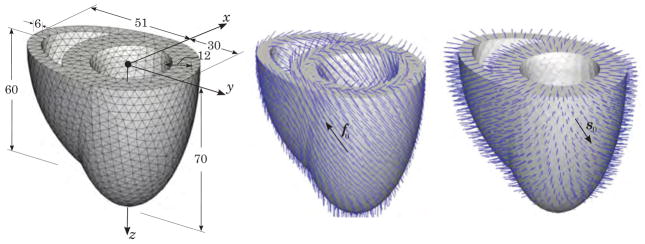
The geometry and discretization of a generic heart model generated by truncated ellipsoids. All dimensions are in millimeters (left). The position-dependent orientation of the myofibers f₀(X) (middle) and the sheets s₀(X) (right) in .

The values of the material parameters used in the coupled analysis of the generic heart model are given in Table 3. Note that the parameters governing the electrical excitation and the active contraction are dimensionless. This is consistent with the non-dimensional setting introduced through the conversion formulas (51,52). In the conversion, we use the factors β_ϕ = 100 mV, δ_ϕ = −80 mV and β_t = 12.9 ms. These are calibrated to obtain the physiological action potential response ranging from −80 mV to +20 mV as suggested in Aliev and Panfilov (1996).

Table 3.

Values of the material parameters used the analysis

Stress response	a1 = 0.496 kPa, b1 = 7.209 [−], am = 15.193 kPa, bm = 20.417 [−], an = 3.283 kPa, bn = 11.176 [−], ak = 0.662 kPa, bk = 9.466 [−], η = 30 kPa
Active Contraction	q = 0.1 [−], k = 0.1 [−], β = 10 [−], ${\lambda }_{max}^{\mathrm{a}}=0.3[-]$
Excitation	a = 0.01 [−], b = 0.15 [−], c = 8 [−]
	γ = 0.002 [−], μ1 = 0.2 [−], μ2 = 0.3 [−]
	Gs = 0 [−], ϕs = 0.6 [−]
Conduction	diso = 1 mm2/ms, dani = 0.1 mm2/ms

The material parameters controlling the passive stress response have been obtained by fitting the passive shear experiments on pig hearts by Dokos et al. (2002), see also Göktepe et al. (2011) for details of the parameter identification. The active stress and active contraction parameters have been calibrated to generate about 50% volume reduction during systole. The parameters governing the electrical excitation have been adopted from Kotikanyadanam et al. (2010). The conduction parameters have been calibrated to limit the total simulation time to nearly 450 ms, which corresponds to the duration of the systolic phase and the part of the diastolic phase of the heart beat. For the sake of simplicity, we neglect the mechano-electrical coupling term by setting G_s = 0 in our numerical analysis. The initial transmembrane potential throughout the model is set to the resting value Φ₀ = −80 mV except for the nodes located at the top base of the dividing wall, the septum. The elevated initial value Φ₀ = −10 mV of the transmembrane potential is assigned to the nodes in this region to trigger the excitation of the heart. We have used a uniform step size of Δt = 3 ms throughout the analysis.

The results of the numerical calculations have been depicted in Figure 11 for the systolic contraction phase and in Figure 12 for the diastolic relaxation phase. The snapshots taken at different instants of the simulation and depicted in the first and second rows of Figures 11 and 12 illustrate the action potential contours in the solid model and the two cross-sectional slices, respectively. The excitation at the top of the septum generates a depolarization front, which travels from the location of stimulation throughout the entire heart, initiating the contraction of the myocytes, see the snapshots in Figure 11. We observe that the contraction of myocytes gives rise to the upward motion of the apex. This upward motion is accompanied by the physiologically observed wall thickening and the overall twisting of the heart. To appreciate these phenomena better, the two cross-sectional slices are presented in the complementary images shown in the second rows of Figures 11 and 12. Undoubtedly, it is the heterogeneous distribution of myocyte orientation that yields this physiological response through the non-uniform contraction of myofibers. Apart from the action potential contours depicted in the first and second rows of Figures 11 and 12, the panels in the third and fourth rows of Figures 11 and 12 illustrate the active ${\tau }_{\text{ff}}^{\mathrm{a}}$ and passive ${\tau }_{\text{ff}}^{\mathrm{p}}$ stress components in the deformed fiber directions, respectively. Comparing the active stress (third rows) and the passive stress (fourth rows) contours with the excitation contours (first rows), we observe the physiological delay in contraction during systole (Figure 11) and in relaxation during diastole (Figure 12). Moreover, we also note that the active fiber stresses are predominantly tensile, while the passive stresses are mostly compressive. As expected, stresses concentrate at base where the displacement degrees of freedom are restrained. Since we do not account for the ventricular pressure evolution within the chambers, the passive stress response is mainly restricted to compression. The incorporation of the ventricular pressure within the chambers might result in also the tensile passive stress regions especially during diastole.

Figure 11.

Coupled excitation-induced contraction of the generic heart model. Snapshots of the deformed model depict the action potential contours at different stages of depolarization. The lines denote the spatial orientation f of contractile myofibers (first row). The two cross-sectional slices in the translucent images in the second row favorably demonstrate the wall thickening and the twisting motion of the heart. The panels in the third and fourth rows illustrate the active ${\tau }_{\text{ff}}^{\mathrm{a}}$ and passive ${\tau }_{\text{ff}}^{\mathrm{p}}$ stress components in the deformed fiber directions, respectively.

Figure 12.

Coupled excitation-induced contraction of the generic heart model. Snapshots of the deformed model depict the action potential contours at different stages of repolarization. The lines denote the spatial orientation f of contractile myofibers (first row). The two cross-sectional slices in the translucent images in the second row favorably demonstrate the wall thickening and the twisting motion of the heart. The panels in the third and fourth rows illustrate the active ${\tau }_{\text{ff}}^{\mathrm{a}}$ and passive ${\tau }_{\text{ff}}^{\mathrm{p}}$ stress components in the deformed fiber directions, respectively.

7. Concluding Remarks

In this contribution, we have proposed a micro-structurally based new kinematic and energetic approach to cardiac electromechanics that combines the active-stress and the active-strain models under a unified framework. Hence, the proposed formulation can be considered as generalization of the active-stress and active-strain models where the pros of the distinct approaches have been incorporated. For this purpose, the deformation gradient has been multiplicatively decomposed into the active and passive parts. The active part of the deformation gradient has been considered to be dependent upon the intracellular calcium concentration that is assumed to evolve with the transmembrane potential through an ordinary differential equation. Thus, the calcium concentration enters the formulation as an internal variable. Moreover, the intrinsically anisotropic, active micro-structure of cardiac tissue has been incorporated through the anisotropic representation of the active part of the deformation gradient. In contrast to the active-strain models suggested in the literature, stress-producing free energy function has been additively decomposed into passive and active parts thereby recovering the additively split stress representation of the active-stress models. In this context, the proposed formulation can be conceived as the generalization of the active-stress and active-strain models hitherto suggested in the literature. As opposed to the most of the models of cardiac electromechanics where the operator splitting methods have been devised, the proposed constitutive model has been numerically treated within the recently proposed, fully implicit, entirely finite-element-based coupled framework. It has been shown that the proposed formulation can be successfully used to simulate the fully coupled three-dimensional excitation-contraction of a generic heart model. With only minor, modular modifications in the particular mechanism of excitation and the muscle organization, our generalized Hill model is broadly applicable to simulate not only cardiac muscle but also smooth muscle and skeletal muscle. Calibrated kinematically through actin-myosin cross bridging, the proposed model can provide fundamental insight into dysregulated excitation-contraction coupling in various diseases such as gastrointestinal track disorders, vascular disorders, neuromuscular diseases, spasticity, or heart disease. Note that the more unified or more dispersed organization of different muscle types can be readily accounted for in the proposed kinematic framework by means of fiber distribution functions with parameters tuned for a particular muscle type of interest. Similarly, the different excitation mechanisms and distinct types of passive response of the specific muscle tissue can be incorporated in the proposed model by adapting the constitutive equations, specified in Section 5. However, the general structure of the proposed approach is so modular that these changes involve only local modifications within the constitutive driver. We leave these extensions out of the current work and plan to elaborate on them in our follow-up works.

References

- Aliev RR, Panfilov AV. A simple two-variable model of cardiac excitation. Chaos, Solitons and Fractals. 1996;7:293–301. [Google Scholar]
- Ambrosi D, Arioli G, Nobile F, Quarteroni A. Electromechanical coupling in cardiac dynamics: The active strain approach. SIAM Journal on Applied Mathematics. 2011;71:605–621. [Google Scholar]
- Ambrosi D, Pezzuto S. Active stress vs. active strain in mechanobiology: Constitutive issues. Journal of Elasticity. 2011;107:199–212. [Google Scholar]
- Ask A, Menzel A, Ristinmaa M. Electrostriction in electro-viscoelastic polymers. Mechanics of Materials. 2012a;50:9– 21. [Google Scholar]
- Ask A, Menzel A, Ristinmaa M. Phenomenological modeling of viscous electrostrictive polymers. International Journal of Non-Linear Mechanics. 2012b;47:156– 165. [Google Scholar]
- Beeler GW, Reuter H. Reconstruction of the action potential of ventricular myocardial fibres. The Journal of Physiology. 1977;268:177210. doi: 10.1113/jphysiol.1977.sp011853. [DOI] [PMC free article] [PubMed] [Google Scholar]
- Bers DM. Cardiac excitation contraction coupling. Nature. 2002;415:198–205. doi: 10.1038/415198a. [DOI] [PubMed] [Google Scholar]
- Cherubini C, Filippi S, Nardinocchi P, Teresi L. An electromechanical model of cardiac tissue: Constitutive issues and electrophysiological effects. Progress in Biophysics and Molecular Biology. 2008;97:562–573. doi: 10.1016/j.pbiomolbio.2008.02.001. [DOI] [PubMed] [Google Scholar]
- Clayton RH, Panfilov AV. A guide to modelling cardiac electrical activity in anatomically detailed ventricles. Progress in Biophysics and Molecular Biology. 2008;96:19–43. doi: 10.1016/j.pbiomolbio.2007.07.004. [DOI] [PubMed] [Google Scholar]
- Dal H, Göktepe S, Kaliske M, Kuhl E. A fully implicit finite element method for bidomain models of cardiac electrophysiology. Computer Methods in Biomechanics and Biomedical Engineering. 2012;15:645–656. doi: 10.1080/10255842.2011.554410. [DOI] [PubMed] [Google Scholar]
- Dal H, Göktepe S, Kaliske M, Kuhl E. A fully implicit finite element method for bidomain models of cardiac electromechanics. Computer Methods in Applied Mechanics and Engineering. 2013;253:323– 336. doi: 10.1016/j.cma.2012.07.004. [DOI] [PMC free article] [PubMed] [Google Scholar]
- Dokos S, Smaill BH, Young AA, LeGrice IJ. Shear properties of passive ventricular myocardium. American Journal of Physiology - Heart and Circulatory Physiology. 2002;283:H2650–H2659. doi: 10.1152/ajpheart.00111.2002. [DOI] [PubMed] [Google Scholar]
- Doyle TC, Ericksen JL. Nonlinear elasticity. In: Dryden HL, von Kármán T, editors. Advances in Applied Mechanics. Vol. 4. Academic Press; New York: 1956. pp. 53–116. [Google Scholar]
- Eriksson TSE, Prassl AJ, Plank G, Holzapfel GA. Influence of myocardial fiber/sheet orientations on left ventricular mechanical contraction. Mathematics and Mechanics of Solids. 2013a doi: 10.1177/1081286513485779. in press. [DOI] [Google Scholar]
- Eriksson TSE, Prassl AJ, Plank G, Holzapfel GA. Modeling the dispersion in electromechanically coupled myocardium. International Journal for Numerical Methods in Biomedical Engineering. 2013b doi: 10.1002/cnm.2575. in press. [DOI] [PMC free article] [PubMed] [Google Scholar]
- Fitzhugh R. Impulses and physiological states in theoretical models of nerve induction. Biophysical Journal. 1961;1:455–466. doi: 10.1016/s0006-3495(61)86902-6. [DOI] [PMC free article] [PubMed] [Google Scholar]
- Göktepe S. In: Fitzhugh-Nagumo equation. Engquist B, editor. Springer; 2013. To appear in Encyclopedia of Applied and Computational Mathematics. [Google Scholar]
- Göktepe S, Acharya SNS, Wong J, Kuhl E. Computational modeling of passive myocardium. International Journal for Numerical Methods in Biomedical Engineering. 2011;27:1–12. doi: 10.1002/cnm.2565. [DOI] [PMC free article] [PubMed] [Google Scholar]
- Göktepe S, Kuhl E. Computational modeling of cardiac electrophysiology: A novel finite element approach. International Journal for Numerical Methods in Engineering. 2009;79:156–178. doi: 10.1002/cnm.2565. [DOI] [PMC free article] [PubMed] [Google Scholar]
- Göktepe S, Kuhl E. Electromechanics of the heart: a unified approach to the strongly coupled excitation-contraction problem. Computational Mechanics. 2010;45:227–243. [Google Scholar]
- Göktepe S, Menzel A, Kuhl E. Micro-structurally based kinematic approaches to electromechanics of the heart. In: Holzapfel GA, Kuhl E, editors. Computer models in Biomechanics. From Nano to Macro. chapter 13. Springer Science+Business Media; Dordrecht: 2013. pp. 175–187. [Google Scholar]
- Göktepe S, Wong J, Kuhl E. Atrial and ventricular fibrillation: computational simulation of spiral waves in cardiac tissue. Archive of Applied Mechanics. 2010;80:569–580. [Google Scholar]
- Hill AV. The heat of shortening and the dynamic constants of muscle. Proceedings of the Royal Society of London Series B - Biological Sciences. 1938;126:136–195. doi: 10.1098/rspb.1949.0019. [DOI] [PubMed] [Google Scholar]
- Hill AV. First and Last Experiments in Muscle Mechanics. Cambridge University Press; 1970. [Google Scholar]
- Hodgkin A, Huxley A. A quantitative description of membrane current and its application to excitation and conduction in nerve. J Physiol. 1952;117:500–544. doi: 10.1113/jphysiol.1952.sp004764. [DOI] [PMC free article] [PubMed] [Google Scholar]
- Holzapfel GA, Ogden RW. Constitutive modelling of passive myocardium: a structurally based framework for material characterization. Philosophical Transactions Series A, Mathematical, Physical, and Engineering Sciences. 2009;367:3445–3475. doi: 10.1098/rsta.2009.0091. [DOI] [PubMed] [Google Scholar]
- Katz AM. Physiology of the Heart. Lippincott Williams & Wilkins; 2011. [Google Scholar]
- Keener JP, Sneyd J. Mathematical Physiology. Springer; New York: 1998. [Google Scholar]
- Keldermann R, Nash M, Panfilov A. Pacemakers in a Reaction-Diffusion mechanics system. Journal of Statistical Physics. 2007;128:375–392. [Google Scholar]
- Klabunde RE. Cardiovascular Physiology Concepts. Lippincott Williams & Wilkins; 2005. [Google Scholar]
- Kohl P, Hunter P, Noble D. Stretch-induced changes in heart rate and rhythm: Clinical observations, experiments and mathematical models. Progress in Biophysics and Molecular Biology. 1999;71:91–138. doi: 10.1016/s0079-6107(98)00038-8. [DOI] [PubMed] [Google Scholar]
- Kotikanyadanam M, Göktepe S, Kuhl E. Computational modeling of electrocardiograms: A finite element approach towards cardiac excitation. International Journal for Numerical Methods in Biomedical Engineering. 2010;26:524–533. doi: 10.1002/cnm.2565. [DOI] [PMC free article] [PubMed] [Google Scholar]
- Kröner E. Allgemeine Kontinuumstheorie der Versetzungen und Eigenspannungen. Archive for Rational Mechanics and Analysis. 1960;4:273–334. [Google Scholar]
- Lafortune P, Ars R, Vázquez M, Houzeaux G. Coupled electromechanical model of the heart: Parallel finite element formulation. International Journal for Numerical Methods in Biomedical Engineering. 2012;28:72–86. doi: 10.1002/cnm.1494. [DOI] [PubMed] [Google Scholar]
- Lee EH. Elastic–plastic deformation at finite strain. ASME Journal of Applied Mechanics. 1969;36:1–6. [Google Scholar]
- Levy MN, Koeppen BM, Stanton BA. Berne & Levy Principles of Physiology. Elsevier Science Health Science Division; 2006. [Google Scholar]
- Luo CH, Rudy Y. A model of the ventricular cardiac action potential. depolarization, repolarization, and their interaction. Circulation Research. 1991;68:1501–1526. doi: 10.1161/01.res.68.6.1501. [DOI] [PubMed] [Google Scholar]
- Menzel A. A fibre reorientation model for orthotropic multiplicative growth. Biomechanics and Modeling in Mechanobiology. 2007;6:303–320. doi: 10.1007/s10237-006-0061-y. [DOI] [PubMed] [Google Scholar]
- Menzel A, Steinmann P. On the spatial formulation of anisotropic multiplicative elasto-plasticity. Computer Methods in Applied Mechanics and Engineering. 2003a;192:3431–3470. [Google Scholar]
- Menzel A, Steinmann P. A view on anisotropic finite hyper-elasticity. European Journal of Mechanics - A/Solids. 2003b;22:71–87. [Google Scholar]
- Nagumo J, Arimoto S, Yoshizawa S. An active pulse transmission line simulating nerve axon. Proceedings of the IRE. 1962;50:2061–2070. [Google Scholar]
- Nardinocchi P, Teresi L. On the active response of soft living tissues. Journal of Elasticity. 2007;88:27–39. [Google Scholar]
- Nash MP, Panfilov AV. Electromechanical model of excitable tissue to study reentrant cardiac arrhythmias. Progress in Biophysics and Molecular Biology. 2004;85:501–522. doi: 10.1016/j.pbiomolbio.2004.01.016. [DOI] [PubMed] [Google Scholar]
- Nickerson D, Nash M, Nielsen P, Smith N, Hunter P. Computational multiscale modeling in the IUPS physiome project: Modeling cardiac electromechanics-Author bios. Systems Biology. 2006:50. [Google Scholar]
- Niederer SA, Smith NP. An improved numerical method for strong coupling of excitation and contraction models in the heart. Progress in Biophysics and Molecular Biology. 2008;96:90–111. doi: 10.1016/j.pbiomolbio.2007.08.001. [DOI] [PubMed] [Google Scholar]
- Nielsen PM, Grice IJL, Smaill BH, Hunter PJ. Mathematical model of geometry and fibrous structure of the heart. The American Journal of Physiology. 1991;260:H1365–H1378. doi: 10.1152/ajpheart.1991.260.4.H1365. [DOI] [PubMed] [Google Scholar]
- Nobile F, Quarteroni A, RuizBaier R. An active strain electromechanical model for cardiac tissue. International Journal for Numerical Methods in Biomedical Engineering. 2012;28:52–71. doi: 10.1002/cnm.1468. [DOI] [PubMed] [Google Scholar]
- Noble D. A modification of the Hodgkin–Huxley equations applicable to purkinje fibre action and pacemaker potentials. The Journal of Physiology. 1962;160:317–352. doi: 10.1113/jphysiol.1962.sp006849. [DOI] [PMC free article] [PubMed] [Google Scholar]
- Opie LH. Heart Physiology: From Cell to Circulation. Lippincott Williams & Wilkins; 2004. [Google Scholar]
- Panfilov AV, Keldermann RH, Nash MP. Self-organized pacemakers in a coupled reaction-diffusion-mechanics system. Physical Review Letters. 2005;95:258104-1–258014–4. doi: 10.1103/PhysRevLett.95.258104. [DOI] [PubMed] [Google Scholar]
- Pelce P, Sun J, Langeveld C. A simple model for excitation-contraction coupling in the heart. Chaos, Solitons & Fractals. 1995;5:383–391. [Google Scholar]
- Pope AJ, Sands GB, Smaill BH, LeGrice IJ. Three-dimensional transmural organization of perimysial collagen in the heart. Am J Physiol Heart Circ Physiol. 2008;295:H1243–1252. doi: 10.1152/ajpheart.00484.2008. [DOI] [PMC free article] [PubMed] [Google Scholar]
- Pullan AJ, Buist ML, Cheng LK. Mathematical Modeling the Electrical Activity of the Heart. World Scientific; Singapore: 2005. [Google Scholar]
- Rohmer D, Sitek A, Gullberg GT. Reconstruction and visualization of fiber and laminar structure in the normal human heart from ex vivo diffusion tensor magnetic resonance imaging (DTMRI) data. Investigative Radiology. 2007;42:777–789. doi: 10.1097/RLI.0b013e3181238330. [DOI] [PubMed] [Google Scholar]
- Rossi S, Ruiz-Baier R, Pavarino LF, Quarteroni A. Orthotropic active strain models for the numerical simulation of cardiac biomechanics. International Journal for Numerical Methods in Biomedical Engineering. 2012;28:761–788. doi: 10.1002/cnm.2473. [DOI] [PubMed] [Google Scholar]
- Sachse FB. Computational Cardiology: Modeling Of Anatomy, Electrophysiology, and Mechanics. Springer Verlag; 2004. [Google Scholar]
- Sermesant M, Rhode K, Sanchez-Ortiz G, Camara O, Andriantsimiavona R, Hegde S, Rueckert D, Lambiase P, Bucknall C, Rosenthal E, Delingette H, Hill D, Ayache N, Razavi R. Simulation of cardiac pathologies using an electromechanical biventricular model and XMR interventional imaging. Medical Image Analysis. 2005;9:467–480. doi: 10.1016/j.media.2005.05.003. [DOI] [PubMed] [Google Scholar]
- Sidoroff F. Un modèle viscoélastique non linéaire avec configuration intermédiaire. Journal de Mécanique. 1974;13:679–713. [Google Scholar]
- Stålhand J, Klarbring A, Holzapfel G. A mechanochemical 3D continuum model for smooth muscle contraction under finite strains. Journal of Theoretical Biology. 2011;268:120–130. doi: 10.1016/j.jtbi.2010.10.008. [DOI] [PubMed] [Google Scholar]
- Tusscher KHWJT, Panfilov AV. Modelling of the ventricular conduction system. Progress in Biophysics and Molecular Biology. 2008;96:152–170. doi: 10.1016/j.pbiomolbio.2007.07.026. [DOI] [PubMed] [Google Scholar]
- Wong J, Göktepe S, Kuhl E. Computational modeling of electrochemical coupling: A novel finite element approach towards ionic models for cardiac electrophysiology. Computer Methods in Applied Mechanics and Engineering. 2011;200:3139–3158. [Google Scholar]
- Wong J, Göktepe S, Kuhl E. Computational modeling of chemo-electromechanical coupling: A novel implicit monolithic finite element approach. International Journal for Numerical Methods in Biomedical Engineering. 2013;29:1104–1133. doi: 10.1002/cnm.2565. [DOI] [PMC free article] [PubMed] [Google Scholar]