A Computational Framework for Heparan Sulfate Sequencing Using High-resolution Tandem Mass Spectra

Abstract

Heparan sulfate (HS) is a linear polysaccharide expressed on cell surfaces, in extracellular matrices and cellular granules in metazoan cells. Through non-covalent binding to growth factors, morphogens, chemokines, and other protein families, HS is involved in all multicellular physiological activities. Its biological activities depend on the fine structures of its protein-binding domains, the determination of which remains a daunting task. Methods have advanced to the point that mass spectra with information-rich product ions may be produced on purified HS saccharides. However, the interpretation of these complex product ion patterns has emerged as the bottleneck to the dissemination of these HS sequencing methods. To solve this problem, we designed HS-SEQ, the first comprehensive algorithm for HS de novo sequencing using high-resolution tandem mass spectra. We tested HS-SEQ using negative electron transfer dissociation (NETD) tandem mass spectra generated from a set of pure synthetic saccharide standards with diverse sulfation patterns. The results showed that HS-SEQ rapidly and accurately determined the correct HS structures from large candidate pools.

Heparan sulfate (HS)¹ is required for all aspects of physiology in metazoan cells and tissues (1–3). As a subclass of glycosaminoglycans (GAGs), HS consists of repeating disaccharide units [-4-(GlcA-β/IdoA-α)-1,4-GlcNAc(NS)-α-], where GlcA/IdoA may undergo 2-O-sulfation, and GlcNAc may undergo N-deacetylation (free -NH₂), N-sulfation, 6-O-sulfation, and in rare cases, 3-O-sulfation (1, 2). HS chains bind covalently to core proteins via a tetrasaccharide linker to a serine residue, and form heparan sulfate proteoglycans (HSPGs). The HS chains on HSPG bind non-covalently to growth factors, morphogens, chemokines, cytokines, and other molecules, and regulate biological activities including cell signaling, cell migration, and remodeling of the extracellular matrix (ECM) (1, 3–5).

Spatial and temporal regulation of the activities of HS biosynthetic enzymes results in mature HS structure that varies according to the biological context. Mature HS chains consist of domains of high, low, and intermediate sulfation respectively, the organization of which varies according to cell type and developmental state. Moreover, variation of chain length and modification patterns associated with different biological sources adds complexity to the HS chains (6). The diversity of HS structures and different levels of binding specificity with multiple protein ligands suggests a physiological mechanism of cellular responses to growth factor stimuli. A well-studied case is the highly sulfated pentasaccharide sequence within heparin that binds antithrombin (AT)-III specifically and regulates blood coagulation process. This pentasaccharide motif contains eight sulfate substituents, including a 3-O-sulfate group, each of which is required for high affinity binding (7–9). Moreover, studies on HS-binding proteins, including fibroblast growth factors (FGF) (10–13), sonic hedgehog (14), vascular endothelial growth factor (VEGF) (15, 16), glial cell line-derived neurotrophic factor (GDNF) (17), chemokines (18), and Wnt (19), demonstrate the importance of sulfation patterns of HS chains in determining the binding specificity between HS, growth factors, and growth factor receptors, and illustrate the potential of developing HS-based drugs and therapeutics (20–23). In this context, effective methods for identifying sulfation patterns on HS chains are in high demand.

The development of experimental methods over the past few years has turned the prospect of HS sequencing into reality (24–27). Recent breakthroughs in chemoenzymatic synthesis of HS with specified sulfation positions have removed roadblocks in designing substrates with desired properties (28). Meanwhile, new tandem mass spectrometric dissociation techniques are now capable of identifying sulfation patterns of some GAG oligosaccharides directly (29, 30). In particular, electron detachment dissociation (EDD) (31) and negative electron transfer dissociation (NETD) (32, 33) techniques generate informative spectra that include rich glycosidic-bond and cross-ring cleavages while maintaining the intact sulfation information. It is also possible to suppress losses of sulfate groups in collision-induced dissociation (CID) tandem mass spectra by derivatizing HS saccharides (34) or by replacing acidic protons with metal cations (35, 36). However, all tandem mass spectra of highly sulfated HS saccharides display useful backbone dissociation combined with some degree of sulfate losses. This gives rise to a multiplicity of product ions with either intact or reduced sulfate numbers, the interpretation of which limits the dissemination of these techniques. It is thus necessary to develop commensurate computational methods to meet the challenges of these new techniques, which will promote the systematic study of the in vitro and in vivo effects of HS fine structure on physiological activities.

In 2005, Saad et al. developed the spreadsheet-based heparin sequencing tool HOST using enzymatic digestion and a CID ESI-MSⁿ approach (37). HOST built oligosaccharide sequences based on similarity analysis that compares tandem mass spectra of disaccharide units produced from the saccharide in question against those acquired from the intact saccharide. Methods have advanced since that time and now allow determination of sulfation and acetylation directly from tandem mass spectra without separate enzymatic digestion. A computational simulation method was also explored to predict the fine structure and domain organization of HS sequence using information from enzymatic digestion and Golgi-based biosynthetic rules (38). This model produced an “average” HS chain statistically and is valuable for guiding the selection of candidate sequences, yet it failed to pinpoint the positions of sulfate groups for a specific chain. The public tool Glycoworkbench (39–41) was also developed to facilitate the assignment of monoisotopic peaks in tandem mass spectra of glycans, but it aided little in the identification of sulfated sites on the sequence scale.

In principle, there is no significant difference between sequencing HS saccharides and other compound classes from tandem mass spectra. The precursor mass identifies a finite set of candidate sequences either dependent or independent of biosynthetic rules. The information contained in the tandem mass spectra then reduces candidate possibilities to an extent commensurate with the quality of the data. Depending on whether a knowledgebase is required for generating candidate sequences, tandem MS sequencing methods are divided into database searching and de novo sequencing. De novo sequencing (42) does not rely on a database of previously identified structures, and therefore is preferred for HS sequencing. One type of de novo sequencing method is based on the spectrum graph model (43–48), which converts the sequencing problem into finding an optimal path by connecting the product ion ladder from one terminal to the other. In this process, mass differences establish the connections between peaks. HS chains consist of alternately repeating HexA and HexN residues with acetate and sulfate groups as variable substituents. This means that neighboring product ions may correspond to monosaccharide, or monosaccharide plus substituents. Because sulfate losses occur, the number of neighboring product ions is increased. In addition, random product ions may produce identical mass differences. A naive method (42), such as PEAKS (49), scores favored product ions, and selects candidate sequences with the highest accumulative scores. This method usually relies on the assumption of instrument-specific ion types, and peaks with ambiguous assignments may affect its performance.

For HS, the size of the sequence space is a combinatorial function that depends on the oligosaccharide backbone and numbers of acetate/sulfate groups. For example, a hexasaccharide with composition [1, 2, 3, 1, 6] ([ΔHexA, HexA, GlcN, Ac, SO₃]) gives rise to 1386 isomers, whereas a 14-mer oligosaccharide with composition [0, 7, 7, 2, 5] produces 1,381,380 theoretical sequences. Sampling methods may speed up the searching process, but the resulting local maximum and convergence problems pose additional burdens on configuring reasonable searching/scoring schemes. Even with efficient limitation of the search space, it may still be difficult to distinguish the true sequence from candidate sequences via sequence scores, because the regions with incorrect sulfate/acetate numbers may be supported by falsely assigned product ions because of product ion assignment ambiguity.

The HS sequencing problem can be considered as finding the best way to distribute fixed numbers of acetate/sulfate groups along the precursor sequence. The precursor mass usually uniquely determines the HS composition, i.e. the counts of monosaccharide residues, sulfate, and acetate groups (Fig. 1A), whereas the counts of monosaccharide residues implicitly determines the sequence of monosaccharide residues and therefore the sequence of candidate acetylation/sulfation sites along the precursor sequence. In this sense, we can rephrase the HS sequence problem as finding the best way to distribute fixed number of acetate/sulfate groups among a fixed set of candidate acetylation/sulfation sites.

Fig. 1.

Summary of basic concepts in HS-SEQ. A hexasaccharide [1, 2, 3, 1, 6] ([ΔHexA, HexA, GlcN, Ac, SO₃]) is used to demonstrate the concepts used in HS-SEQ. A, The hexasaccharide sequence illustrated by cartoon symbols. Each monosaccharide has a unique ID. B, Visual representation of the hexasaccharide sequence in HS-SEQ. Two types of modification (substitution) occur on the sequence: acetylation (Ac) and sulfation (SO₃). Each modification type corresponds to a set of candidate modification sites, and a modification distribution, which appends a local likelihood value to each candidate site. C, Visual representation of assignment in HS-SEQ. Each assignment provides structural information in terms of subsets of candidate modification sites as well as the associated modification numbers. D, Assignment helps update the modification distribution. The original modification numbers are denoted by red text and the new numbers deduced from the assignment are denoted by blue text. The added structural information from the assignment updates the local regions of the modification distributions (the updated regions is marked by dashed squares).

We clarify several terms (Fig. 1B) here in order to facilitate the discussion. We use modification to represent acetylation/sulfation, the locations of which are uncertain on the precursor sequence before prediction. In contrast, we consider derivatization at the reducing-end as an integrated part of the precursor backbone because there is no uncertainty of its location. Accordingly, a candidate modification site represents a particular position on a particular monosaccharide residue where the modification may occur, and modification number stands for the count of the modification occurrence. The solution is a list of modification distributions that specify how the given numbers of modifications are distributed among all the candidate modification sites. Each modification type corresponds to a modification distribution, and the sum of the distribution equals the modification number defined in the precursor composition.

The concepts of candidate modification sites and modification number serve as the building blocks for the whole framework of HS-SEQ. For a given peak, we denote each structural interpretation of a peak (the ion type, cleavage position, neutral loss, and modification numbers, e.g. Y₃ - H₂O + 1Ac + 3SO₃) as an assignment. Each assignment in essence contributes structural information regarding the covered candidate modification sites and modification numbers (Fig. 1C). In this sense, each assignment defines a subproblem of the original HS sequencing problem, which serves to update the global modification distributions to finer resolution (Fig. 1D). Moreover, a terminal assignment describes an assignment containing an intact monosaccharide residue of either the reducing end (RE) or non-reducing end (NRE), and an internal assignment describes an assignment containing no intact RE or NRE residue. For each modification type, we use assignment graph to describe the relationship between assignments. In the graph, the node represents an assignment and the edge represents the inclusion relationship of candidate modification sites of two assignments.

In order to identify the HS sequence, the intuitive way is to map the mass values of peaks to assignments (spectra interpretation), and collect the structural information of assignments to deduce the modification distributions of the precursor sequence (sequence assembly). Ambiguity occurs when a single mass value corresponds to multiple assignments, and different assignments produce inconsistent structural information regarding the precursor sequence (Fig. 2A). In essence, the data ambiguity problem is all about confusing information of the candidate modification sites and/or modification numbers (Fig. 2B). As we have seen, nearly all the concepts and difficulties in HS sequencing can be rephrased in terms of candidate modification sites and modification number. Based on the rephrased framework, we developed a de novo sequencing algorithm, HS-SEQ, to address the problem of HS sequencing.

Fig. 2.

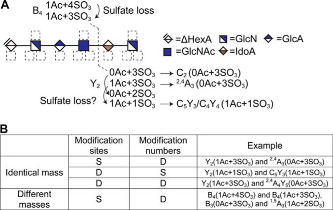
Data ambiguity in HS sequencing. A, Assignments of B₄ and Y₂ on a hexsaccharide with composition [1, 2, 3, 1, 6]. Some Y₂ assignments have incompatible modification numbers with the B₄ assignments. For example, B₄ (1Ac+4SO₃) and Y₂ (1Ac+3SO₃) cannot co-exist because the total number of Ac on the sequence is only 1. Alternative assignments are suggested after the arrows. For example, Y₂ (0Ac+2SO₃) can be considered as Y₂ (0Ac+3SO₃) with sulfate loss, or C₂(0Ac+3SO₃) with sulfate loss. B, Classes of data ambiguity. Assignments with either the same mass values (isomeric or isobaric) or different mass values can cause ambiguity, and the ambiguity in essence is the ambiguity of the candidate modification sites and/or associated modification number. “S” denotes “same” and “D” means “different”.

As shown in Fig. 3A, the sequencing task in HS-SEQ consisted of two steps: (1) the prediction of the distribution of acetate groups, taking into account the data ambiguity; and (2) the prediction of the distributions of sulfate groups, a step divided into sulfate numbers on each monosaccharide residue and exact sulfation positions within residues. Sulfate loss was considered during this step. Fig. 3B illustrates how an assignment connected to others and contributed to updating the modification distribution. HS-SEQ organized assignments by their respective confidence values and sequentially inserted the assignments into the assignment graph. The insertion of each assignment further updated the modification distribution. The final modification distribution can be read manually, or converted to a list of top candidate sequences (see supplemental materials section Generation of top candidates).

Fig. 3.

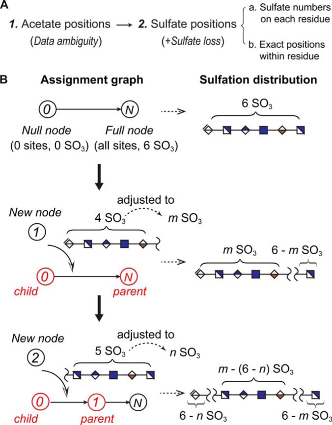
Schema of HS sequencing in HS-SEQ. A, Subtasks in HS sequencing. In HS-SEQ, HS sequencing consists of two basic steps: identification of Ac positions and identification of sulfate positions (sulfate numbers on each residue, and identification of specific sulfate positions on each residue). Data ambiguity is considered for each step, and sulfate loss is considered when identifying sulfate positions. B, Assignment graph connects assignments and generates the modification distribution. The relationship between assignments is visualized by the assignment graph (modification-specific), where the node represents assignment and the edge represents the inclusion relationship of candidate modification sites between assignments. The edge directs the assignment with maximum subset of modification sites (child node) to the assignment with minimum superset of modification sites (parent node). Two nodes are always present in the graph: the null node and the full node. For each new node (assignment), there is always at least one parent node and one child node in the graph. The information of candidate modification sites from the new node helps locate its parent and child in the graph. The information of modification number is adjusted based on confidence estimation of the assignment (discussed in the method section). Each insertion of a node into the graph corresponds to update of local regions on the modification distribution.

We tested HS-SEQ using nine synthetic HS saccharide standards representing a range of chain lengths, modification positions, sulfation degrees, reducing-end derivatization groups, and ion charge states (Fig. 4). The results showed that HS-SEQ accurately recovered the correct HS sequences for 76% (19 out of 25) of the tested tandem mass spectra, and approached the correct sequences for the remainder. For each oligosaccharide sequence, at least 50% of the tandem spectra (each with a different charge state) reported the true sequence as rank 1. Moreover, the scores for the correct HS structures were distinct from their isomeric candidates, and the computation time required for sequencing was usually a few seconds, demonstrating the feasibility of a HS high-throughput sequencing pipeline. The program was developed using the C++ language and is available for download through http://code.google.com/p/glycan-pipeline/. The program currently runs under command line and requires only a few basic arguments (precursor ion m/z, charge state, and input/output file). The program also includes XML configuration files that specify the rest of parameters and their default values. A graphical-user-interface (GUI) version of the program is under development and will be available in future version.

Fig. 4.

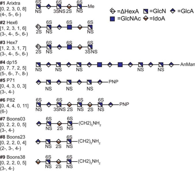
Structures of nine synthetic pure standards for algorithm validation. #1 Arixtra [0, 2, 3, 0, 8] (charge state 4-, 5-, and 6-) was purchased from Organon Sanofi-Synthelabo LLC (West Orange, NJ). #2 Hex6 [1, 2, 3, 1, 6] (charge state 3-, 4-, 5-, and 6-) and #3 Hex7 [1, 2, 3, 1, 7] (charge state 3-, 4-, 5-, and 6-) were purchased from New England BioLabs (Ipswich, MA). #4 dp15 [0, 7, 7, 2, 5] (charge state 5-, 6-, 7-, and 8-), #5 P71 [0, 4, 3, 0, 3] (charge state 3- and 4-) and #6 P82 [0, 4, 4, 0, 11] (charge state 6-) were bio-enzymatically synthesized and were generously provided by Prof. Jian Liu from University of North Carolina, Chapel Hill. Synthetic HS tetrasaccharides #7 Boons03 [0, 2, 2, 0, 4] (charge state 3- and 4-), #8 Boons23[0, 2, 2, 0, 4] (charge state 2-, 3-, and 4-) and #9 Boons38[0, 2, 2, 0, 5] (charge state 3- and 4-) were generously provided by Professor Geert-Jan Boons from the Complex Carbohydrate Research Center at the University of Georgia. Me: methyl, AnMan: 2,5-anhydro-D-mannose, PNP: 4-Nitrophenol.

To the knowledge we have, our work is the first to systematically study the problem of automatic HS sequencing. We showed HS-SEQ's capability in addressing the challenges of data redundancy, data ambiguity, and sulfate loss inherent in tandem mass spectra of HS compound class, and providing production-grade distinctive results.

EXPERIMENTAL PROCEDURES

Data Acquisition and Preprocessing

Tandem mass spectra of the nine synthetic HS saccharides were acquired on a 12-T solariX^TM hybrid Qh-Fourier transform ion cyclotron resonance (FTICR) mass spectrometer (Bruker Daltonics, Bremen, Germany) in NETD (Fig. 4). All HS standards were dissolved in 5% isopropanol, 0.2% ammonia solution to a final concentration of 5 pmol/μl, and infused directly into the mass spectrometer using an Apollo II nanoESI source. The spectra were acquired in the negative ion mode and the instrument parameters were optimized to minimize SO₃ losses. Precursor ions were isolated using a mass-filtering quadrupole and externally accumulated in a hexapole collision cell before tandem MS analysis. For NETD experiments, fluoranthene cation radicals were generated in a chemical ionization source in the presence of argon. Efficient dissociation was ensured by using a reagent accumulation time of up to 500 ms and a reaction time of up to 500 ms. Each transient was acquired with 1m data points, each tandem mass spectrum was acquired by signal averaging up to 100 transients for improved S/N ratio. The instrument was externally calibrated using sodium-TFA clusters before tandem MS experiments.

Peak lists were exported from the spectra using Bruker DataAnalysis 4.2 with the “FTMS” option selected and the signal-to-noise ratio (S/N) threshold set to 0. Each row of the peak lists contained the m/z value, intensity, resolving power and S/N for a given peak. An in-house deconvolution/deisotoping program (see supplemental materials section Deconvolution and deisotoping) was developed to convert the peak lists into lists of monoisotopic neutral masses.

Peak Assignment

The monoisotopic peak list was converted into neutral mass values, and was matched to theoretical fragment mass with a 2 ppm mass error. The theoretical library was constructed from the composition of precursor ion [ΔHexA, HexA, GlcN, Ac, SO₃]. All possible product ions (50) were considered, including types of A, B, C, X, Y, Z, and internal ions generated from multiple cleavages of the HS backbone structure. Neutral mass loss (-H₂O), hydrogen transfer (-H) and all possible numbers of sulfate/acetate groups allowed on the product ions were taken into account. We assumed that for GlcN residues, sulfation may only occur at 2-N, 3-O, and 6-O positions and acetylation at 2-N position, whereas for HexA (GlcA or IdoA) residues, sulfation may occur at the 2-O position. Although it has been suggested that the isomeric uronic acid residues resulted in different fragmentation patterns using EDD (31), the difference has not yet been established as an explicit pattern for automatic recognition from the spectra. Therefore, HS-SEQ did not attempt to distinguish GlcA from IdoA.

Sequence Construction

1. Filtering Redundant Data

A typical assignment of a peak consisted of three parts: product ion type (e.g. B₂, C₃, and ^1,5A₂), composition shift (e.g. -H₂O, -H) and modification numbers for acetate and sulfate groups. Assignments with the same product ion type and the same number of acetate groups were clustered. In other words, each cluster contained assignments with mass values differing only in the equivalent of a combination of neutral mass loss (–H₂O), hydrogen transfer (–H), and sulfate groups. Note that assignments of B- and C-type ions were not differentiated. Similarly, Y- and Z-type ions were clustered together. For example, assignment B₂ (–H₂O, 1Ac + 3SO₃) was clustered with assignment C₂ (–H, 1Ac + 2SO₃), but not with assignment C₂ (0Ac + 1SO₃) because of the different acetate numbers they hold. For each cluster, the assignments with the highest number of sulfate groups were selected to represent the cluster. If more than one assignment had the highest sulfate number in one cluster, HS-SEQ chose the one by the neutral mass shift in order of priority: no shift > -H₂O > +H/–H > -H₂O +H/–H. The number of +H/–H was set to be from 0 to 2 by default.

The clustering procedure removed redundant and/or irrelevant structural information (e.g. composition shift, sulfate losses) of the assignments. As a result, each selected assignment represented an independent observation of a sub-structure of the precursor. Note that the number of acetate groups, instead of sulfate groups, was included for clustering assignments. This was because of the ambiguity of modification number caused by acetate group. For example, in sequence #2 [1, 2, 3, 1, 6] (Fig. 4), a peak assigned to ^0,2A₅ (1Ac + nSO₃) can be equivalently assigned to B₅ (0Ac + nSO₃), whereas a peak assigned to C₅ (1Ac + nSO₃) can be assigned to ^2,4A₆ (0Ac + nSO₃). These ambiguous assignments had the same candidate Ac sites but different Ac numbers, and could not be differentiated from the mass value. In contrast, assignment ambiguity rarely involved the number of sulfate groups, but loss of sulfate group during dissociation may lead to misunderstanding of the sequence. By selecting the assignment with the highest number of sulfate groups within a cluster, the risk of misinterpretation caused by sulfate loss was reduced.

Another clustering procedure in HS-SEQ to reduce the risk of sulfate-loss will be described in step 4.

For each modification type, the algorithm went over step 2 - step 4 to construct the corresponding modification distribution.

2. Estimating Data Ambiguity

Only terminal assignments were considered for building the sequence, but internal assignments were used for estimating the risk of mis-assignment. For each modification type, the likelihood of correctly assigning a peak as an terminal assignment is assessed via uniqueness value p(A), defined as

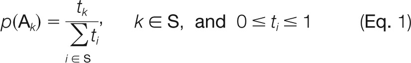whereas S is the indices of isomeric assignments (assignments that correspond to the same mass value, k is the index of a terminal assignment in S, t_k is the weight associated with the cleavage type (e.g. glycosidic-bond cleavage, cross-ring cleavage, and the combinations thereof) of assignment k. For assignments of either glycosidic-bond cleavage or cross-ring cleavage, t_i was set to 1.0; for assignments of internal cleavage type (except double cross-ring cleavage, e.g. AX ion), t_i was set to 0.2; for double cross-ring cleavage, t_i was set to 0 by default, which means assignments of double cross-ring cleavage were ignored. Note that the denominator of the uniqueness value (Eq. 1) was calculated based on assignments with non-redundant information of modification sites and modification number. If assignments of a mass value caused no additional ambiguity (Fig. 2B) regarding the modification sites and modification numbers, they would not be counted into the denominator of the uniqueness value (Eq. 1).

3. Constructing the Assignment Graph

Terminal assignments were organized via an assignment graph model for each modification type (Fig. 3B). Let X denote the set of candidate modification sites of an assignment and S denote the number of sulfate/acetate groups of the same assignment. Node i is a parent of node k, if X_i ⊃ X_k and there is no such node m that X_i ⊃ X_m ⊃ X_k. Conversely, node k is a child of node i. Note that it is possible for a node to have more than one parent/child. For example, nodes representing ^2,4A₃ and ^3,5A₃ are both parents of the node representing B₂ with respect to the sulfation sites. Node i is defined as the complement node of node k if X_k ∪ X_i = Ω, X_k ∩ X_i = ∅ and S_k + S_i = S_precursor, whereas Ω denotes the modification sites of the precursor sequence, ∅ denotes the empty set and S_precursor is the total modification number of the precursor sequence. Conversely, node k is also a complement node of node i, and the two nodes are complementary to each other.

As shown in Fig. 3B, the computation began with two connected dummy nodes, one representing the candidate modification sites and modification number of the precursor ion, and the other representing a virtual node with null modification sites and modification number of 0. For any new assignment, there was always at least one parent and one child in the graph. The terminal assignments were sequentially inserted into the graph by looking for their respective parent and child in the graph, and the insertion order depended on their respective confidence values. The confidence of an assignment relied on several factors: the assignment ambiguity, represented by the uniqueness value p(A) (Eq. 1), and the assignment compatibility with the parent, child, and complement node (if applicable).

The compatibility of assignment k was given by

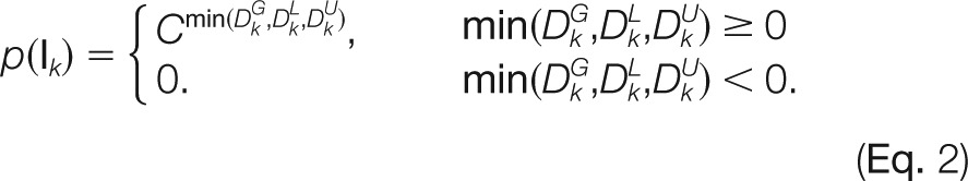where k is the index of a terminal assignment, and C is a constant within [0,1] (0.8 by default). The boundary of the number of sulfate/acetate groups an assignment can carry is mathematically constrained by its parent, child as well as the complement assignment. D^G, D^L, and D^U represent the distances of the modification number of an assignment to the maximal status from different aspects. Constant C regulates the impact of the distance on the assignment compatibility. The rationale behind this formula is that the closer the modification number of an assignment is to the maximum, the more likely the node is to retain the original modification number information. This is especially useful for determining the sulfate distribution because we hope to select assignments that are most likely to retain the intact sulfation information. D^G, D^L, and D^U in (Eq. 2) are given by

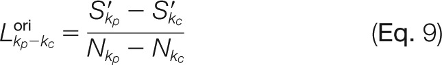
where k is the index of the to-be-inserted node, k_c is the index of the child of node k, k_p is the index of the parent of node k, k' is the index of the complement node of node k, S is the modification number, and N is the number of candidate modification sites. If no complement node of node k has been recorded in the graph, let S_k' = 0. D^G is the distance inferred from a pair of complementary nodes (i.e. distance for golden pair), D^L represents the distance inferred from the child node (i.e. distance for the lower bound), and D^U is the distance inferred from the parent node (i.e. distance for the upper bound).

In the event that more than one candidate parent/child node was present, the most confident one was selected, and its distance values were calculated accordingly.

In order to expand the assignment graph, terminal assignments were sorted descendingly by their uniqueness values p(A) (Eq. 1). In each cycle, assignments with the highest uniqueness values were retrieved. Note that for sulfation distribution, assignments with the same uniqueness value and same modification sites underwent an additional clustering procedure (as described in step 1) so that only the assignment with the highest number of sulfate groups in each cluster was selected. This clustering procedure is useful for grouping nearby assignments covering the same candidate sulfation sites, e.g. B₃ and ^1,5A₃ (see Fig. 2B).

The compatibility (Eq. 2) of assignment k involved two cases: (1) the compatibility with assignments in the current assignment graph (background assignments), denoted as p(I_k^bg), and (2) the compatibility with assignments of the same uniqueness values (peer assignments), denoted as p(I_k^peer). A virtual complement node k′ of node k was forged (if not available), and the confidence value λ of node k was then calculated by:

whereas k is the index of the current node, k' is the index of the complement node of node k, and p(I_k^peer), p(I_k'^peer) represents the compatibility value of node k, node k' in the context of peer assignments (Eq. 2), respectively. Assignments with confidence value of 0 were ignored. The remainding peer assignments were sorted by their confidence values λ (Eq. 6) in a descending order, and sequentially inserted into the assignment graph. Each insertion of a node was accompanied with the insertion of its complement node (either virtual or not).

4. Updating Modification Distribution

With only two dummy nodes in the graph, the modification was equally likely to occur on all possible modification sites along the precursor sequence. The insertion of a node into the assignment graph led to an update of a local region of the modification distribution (Fig. 3B). From the perspective of the assignment graph, the confidence value λ (Eq. 6) was responsible for arranging the order of nodes for insertion into the graph; from the perspective of modification distribution, λ directed the way of updating the distribution. Intuitively, if the confidence value was close to 0, the inserted node had almost no impact on the current modification distribution; if it was close to 1, the modification distribution was updated based on the exact modification number of the assignment (Fig. 1D). Therefore, λ controlled the effect of modification number of an assignment on updating the modification distribution (Fig. 3B). The adjusted or “effective” modification number S′ for assignment k was given by:

whereas k is the index of the inserted node, S denotes the modification number, λ is the confidence value (Eq. 6), and S_k^bg is the background modification number for node k, given by:

where k is the index of the inserted node, k_c is the index of the child of node k, S′ is the effective modification number, N is the number of candidate modification sites and L_kp−kc^ori is the average modification number over the candidate modification sites sandwiched by the parent and child of node k. If the child node or parent node is the dummy node, let S′ = S.

L_kp−kc^ori was given by:

whereas S′ denotes the effective modification number, N is the number of modification sites, k_p is the index of the parent of node k, k_c is the index of the child of node k.

After the insertion, the original modification distribution was updated in the following way: for the subregion demarcated by the node k and its child k_c, the updated average modification number on each candidate modification site, or local modification likelihood, was given by:

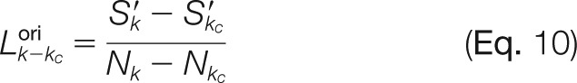Similarly, for subregion demarcated by node k and its parent node k_p, the updated local modification likelihood on each candidate site was also given by:

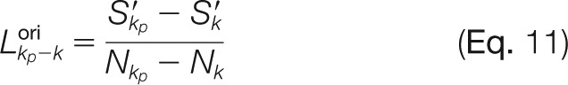As more assignments were inserted into the assignment graph, the modification distribution was sliced into smaller pieces of subregions with the candidate modification sites and adjusted modification numbers specified.

5. Organizing Sequencing Tasks

The acetylation positions were identified first by selecting the most likely candidate acetylation sites based on predicted acetylation distribution. All assignments that reported inconsistent acetate numbers were removed in order to improve the accuracy of predicting sulfation distribution.

Ideally, the presence of cross-ring cleavage product ions facilitates locating the sulfate groups within each residue. In practice, however, cross-ring cleavage product ions were more likely to be associated with sulfate loss. As a result, HS-SEQ might incorrectly distribute the sulfate group(s) within the residue (see supplemental material S1). Fortunately, once the number of sulfate groups on each residue was determined, it was usually possible to deduce the priority of sulfation positions within residues based on the biosynthetic rules of HS (4, 51).

Method Comparison

The performance of HS-SEQ was evaluated using 25 NETD spectra from nine synthesized sequences (Fig. 4). For each spectrum, all theoretical sequences were enumerated (Table I) based on the compositions of the precursor ions, and the prediction cost for each candidate sequence was calculated. Each candidate sequence was virtually represented by modification distributions with only binary likelihood values (0–1), where 0 and 1 denote “unoccupied” and “occupied” position, respectively. The prediction cost for a given candidate sequence was defined as the distance between the binary modification distributions representing the candidate sequence and the modification distributions predicted by HS-SEQ, which was given by

whereas T is the set of modification types (acetylation/sulfation), S(t) is the set of candidate modification sites for modification type t, d_ti is the estimate of modification likelihood from HS-SEQ on site i for modification type t, and k_ti is the binary modification likelihood (0–1) specified by candidate sequence on site i for modification type t. For each spectrum, the average rank and Z-score of the cost value (Eq. 12) of the true sequence were calculated in the background of all candidate sequences. The true sequence was expected to have a good average rank (low prediction cost) and high Z-score (distinct from background).

Table I. Average ranks of the true sequences using HS-SEQ. For each spectrum, the average ranks of the true sequence in the sequence space and residue-based sequence space (M_space) using HS-SEQ were listed.

Sequence (charge)	Rank/Space	M_rank/M_space	Sequence (charge)	Rank/Space	M_rank/M_space
#1 (4-)	12/165	1/25	#5 (3-)	8/286	1/56
#1 (5-)	75/165	4/25	#5 (4-)	2/286	1/56
#1 (6-)	16/165	1/25	#6 (6-)	30.5/4368	1/328
#2 (3-)	26.5/1386	2/216	#7 (3-)	15.5/56	1/12
#2 (4-)	13.5/1386	1/216	#7 (4-)	1.5/56	1/12
#2 (5-)	29.5/1386	1/216	#8 (2-)	6/70	1/14
#2 (6-)	114.5/1386	1/216	#8 (3-)	2.5/70	1/14
#3 (3-)	17.5/990	2/174	#8 (4-)	1.5/70	1/14
#3 (4-)	3.5/990	1/174	#9 (3-)	13.5/56	3/12
#3 (5-)	7.5/990	1/174	#9 (4-)	2/56	1/12
#3 (6-)	12.5/990	1/174
#4 (5-)	1.5/1,381,380	1/98,196
#4 (6-)	1/1,381,380	1/98,196
#4 (7-)	70.5/1,381,380	2/98,196
#4 (8-)	1630.5/1,381,380	3/98,196

The performance of HS-SEQ was compared with two other naïve methods. The first was the coverage method (39, 41), which we defined here as scoring a candidate sequence by calculating the total number of observed unique mass values of product ions explainable by that sequence. Ideally, the most likely sequence should have the highest coverage, and all other sequences should cover only a subset of the mass values. The second naïve method tested was the “golden pair” (GP) (36), which we redefined here as counting the pairs of complementary terminal assignments for a given candidate sequence. Similarly, we assumed that a true sequence should have the highest number of golden pairs.

For native samples derived from biological sources, there was a priority order for sulfation positions within a GlcN residue. Therefore, the performances of a residue-based version of all three methods were also compared, which we denoted as M_Coverage, M_GP and HS-SEQ (M_Cost) methods, respectively. Candidate sequences with no differences in the total number of sulfate groups for each residue were adjusted to have the same score.

HS-SEQ (M_Cost) for a sequence at the residue level was calculated by

whereas T is the set of modification types (acetylation/sulfation), R(t) is the list of monosaccharide residues for modification type t, D_tr is the modification likelihood estimated from HS-SEQ on residue r for modification type t, and K_tr is the summed modification number (nonnegative integer) specified by the candidate sequence on residue r for modification type t. It turns out that the residue-based version is more robust to variation of occupied sulfation sites within each residue. For example, if HS-SEQ produces sulfation likelihood values on sites in a GlcN residue as (2-N: 0.3, 3-O: 0.9, and 6-O: 0.8), and a candidate sequence specifies the sulfation distribution on the same sites as (2-N: 1, 3-O: 0, and 6-O: 1). The original version of the cost function would calculate the squared distance as (0.3 - 1)² + (0.9 - 0)² + (0.8 - 1)² = 1.34, whereas the updated cost function would give (0.3 + 0.9 + 0.8 - 1 - 0 - 1)² = 0.

For M_Coverage, a qualified assignment of cross-ring cleavage type was allowed to carry more sulfate groups than the number on the local region specified by the candidate sequence, as soon as the residue-based constraint of the candidate sequence was met. For example, for candidate sequence in (Fig. 1A), a qualified B₁ assignment can carry up to one sulfate group, and a qualified B₂ assignment can carry up to three sulfate groups. Under the loosened constraint, a ^2,4A₂ assignment can carry at most two sulfate groups, and a ^0,2A₂ assignment up to three sulfate groups. Therefore, a sequence with sulfation at 2-N and 6-O on a GlcN residue counted equally amount of assignments as an isomer sequence with sulfation at 3-O and 6-O on the same GlcN residue, assuming other residues of the two sequences had the same sulfation distribution. The same loosened constraint was applied to M_GP to select qualified assignments for each candidate sequence. The performances (average rank and Z-score) of the three updated methods were then compared. The relationship between the performance and the size of candidate sequence space (background size) for both the original and updated versions of all three methods were also explored.

RESULTS

The preprocessing results are given in supplemental material S2–S3 and the modification distributions reported by HS-SEQ are provided in supplemental material S1. We compared the average ranks of the true sequences using all three methods (Fig. 5A). A low rank value indicated high rank performance. The results suggested that the coverage method was the most stable among the three, and performed best for sequence #2 (charge 3-, 4-, 5-, and 6-), #6 (charge 6-) and #7 (charge 3-). The performance of HS-SEQ (Cost) was close to the coverage method in general, with the exception that it lagged behind for sequence #1 (charge 4-, 5-, and 6-), #2 (charge 5- and 6-) and #6 (charge 6-), whereas it targeted sequence #4 (charge 6-) accurately. The GP method performed poorly for #8 (charge 2- and 3-), #2 (charge 3-, 4-, 5-, and 6-), #6 (charge 6-) and #4 (5-, 6-, 7-, and 8-).

Fig. 5.

Comparison of HS sequencing methods. The performance for coverage method (denoted in black), GP method (denote in blue), HS-SEQ (Cost) (denoted in red) were compared using the 25 NETD spectra. A, Comparison of the average ranks. B, Comparison of the absolute values of Z-scores. C, Comparison of correlations between average rank and background size. D, Comparison of correlations between Z-score and background size. Note that in A, and B, the sequences were sorted in an ascending order by their background size.

The Z-score test (Fig. 5B) provided a measure of the distinction of a true sequence from the background candidates. HS-SEQ (Cost) performed best for sequence #5 (charge 4-) and #4 (5-, 6-, 7-, and 8-). The GP method performed best for #1 (4-, 5-, and 6-), but produced no results for #8 (charge 2-) because of missing observations of golden pairs. The coverage method, the best performer in the average rank test, gave a mediocre performance in the Z-score test. This was not surprising, because ambiguous assignments in HS tandem MS spectra were expected to boost the scores of some candidate sequences. The results showed that HS-SEQ (Cost) gave good Z-scores consistently, especially for sequence #7 (4-, 56 candidates), sequence #9 (4-, 56 candidates), sequence #8 (3-, 70 candidates), sequence #5 (3- ∼ 4-, 286 candidates), #3 (4-, 990 candidates), #6 (6-, 4368 candidates), and #4 (5- ∼ 8-, 1,381,380 candidates).

We also examined the linear correlation between average rank and background size (Fig. 5C). The results showed that the linear correlation was weak for HS-SEQ (Cost) (R² = 0.171), compared with strong correlation for the coverage (R² = 0.563) and GP (R² = 0.505) methods. It was interesting for HS-SEQ (Cost) to have significantly smaller R² value, because a larger background size typically indicates a higher chance for a sequencing algorithm to make mistakes. For sequences of the same background size, HS-SEQ (Cost) tended to generate average ranks with higher variance compared with the naïve methods. This suggests that factors other than the background size may strongly affect the average rank performance of HS-SEQ (Cost). The regression line for HS-SEQ (Cost) (Fig. 5C) had a smaller slope compared with other methods, which also suggests that the average rank from HS-SEQ (Cost) was less affected by the background size. In contrast, all three methods showed strong linear correlations on the relationship between the Z-score and the background size (R² = 0.726 for the coverage method, R² = 0.641 for the GP method and R² = 0.601 for HS-SEQ (Cost)), but the regression line for HS-SEQ (Cost) again was steeper than the lines for the naïve methods. This indicates that HS-SEQ (Cost) had special advantage in identifying the true sequence from the background, especially in the case of large background size. The characteristic distinctiveness of HS-SEQ was highly favorable for automatic HS sequencing.

Close examination of the modification distributions from HS-SEQ (Cost) provided an explanation (see supplemental material S1). Some degrees of sulfate losses were observed with all dissociation methods, including NETD (52). This was more likely to happen for cross-ring cleavages. Although the coverage method considered product ions with sulfate loss, the GP and HS-SEQ (Cost) methods required the presence of product ions with no sulfate loss. Fortunately, the total number of sulfate groups on each residue was usually well maintained in the sulfation distribution generated by HS-SEQ, because glycosidic-bond cleavages surrounding each residue were more likely to retain all sulfate groups. In this sense, by ignoring the relative sulfation positions within GlcN residues, we expected HS-SEQ to perform well even in the average rank test.

We compared the updated version of all three methods (Fig. 6). As expected, the HS-SEQ (M_Cost) method showed great improvement in the average rank test (Fig. 6A) and maintained its excellent Z-score performance (Fig. 6B). Although the M_Coverage method provided comparable performance in the average rank test for most sequences, its suboptimal performance in the Z-score test made it less practical. As shown in supplemental Table S1, HS-SEQ (M_Cost) successfully identified the correct structure as rank 1 for 19 out of 25 (76%) spectra, whereas M_Coverage identified 11 (44%) and M_GP identified 3 (12%). Because nearly all precursor sequences were present in multiple charge states, the supports of each precursor sequence from multiple spectra (each spectrum corresponds to a charge state) were also examined. We defined that if at least 50% of the spectra of the same sequence supported the true sequence as rank 1, then the sequence was correctly identified. The results (supplemental Table S1) showed that HS-SEQ (M_Cost) correctly identified all sequences (100%). In contrast, M_Coverage deduced the correct structure for 66.7% of the sequences (sequence #1, #5, #6, #7, #8, and #9), and M_GP only worked for sequence #1 (representing 11% of the sequences) (see supplemental Table S1).

Fig. 6.

Comparison of updated version of HS sequencing methods. The performance for updated version of the coverage method (M_Coverage, denoted in black), GP method (M_GP, denoted in blue) and HS-SEQ (M_Cost, denoted in red) were compared using the 25 NETD spectra. A, Comparison of the average ranks. B, Comparison of the absolute values of Z-scores. C, Comparison of correlations between average rank and background size. D, Comparison of correlations between Z-score and background size. Note that in A, and B, the sequences were sorted in an ascending order by their background size.

The updated methods showed similar results in the correlation study (Fig. 6C) and (Fig. 6D) as the original methods (Fig. 5C and 5D). In the average rank versus background size test, the linear correlation dropped for all three methods (for HS-SEQ, R² changes from 0.171 to 0.033; for the coverage method, R² from 0.563 to 0.345; for the GP method, R² from 0.505 to 0.400), but the distinction of R² between HS-SEQ (M_Cost) and the other two remained. The linear correlations between the Z-score and the background size were similar for all three methods (R² = 0.697 for HS-SEQ (M_Cost), R² = 0.754 for M_Coverage, and R² = 0.751 for M_GP), albeit the regression line for HS-SEQ (M_Cost) had the steepest slope. This suggests that as the background size grew, HS-SEQ (M_Cost) tended to provide the most distinctive results.

When tied scores were assigned the minimum rank values (see supplemental Table S2), the original versions of the coverage and GP methods assigned the true sequences as rank 1 for most of the tested spectra. However, when tied scores were assigned the maximum rank values, all three methods performed poorly in identifying the true sequences (see supplemental Table S3). Histograms demonstrating the distinctiveness of three methods are given in Fig. 7A and supplemental Figs. S10–S34. The comparison of |Z-score| for all three methods is given in supplemental Table S4.

Fig. 7.

Example demonstrating the performance of HS-SEQ. A, Comparison of histograms of candidate sequence scores using different methods. The calculation was based on tandem mass spectrum from sequence #2 (charge 5-). Red arrow flags the score of the true sequence structure. B, Integration of results from multiple charge states. The modification distributions (bottom left) were calculated using data from sequence #2 (charge 3- ∼ 6-). The modification number on each residue was then mapped to the original oligosaccharide sequence (bottom right). White bar denotes acetylation distribution, gray bar denotes sulfation distribution, and the error bar indicates standard error. Digits beside the vertical solid lines represent the estimated modification number on each residue. Red asterisk indicates the positions where modifications actually occur.

To summarize, HS-SEQ (M_Cost) consistently provided the best performance regarding the average rank and distinctiveness, which enabled confident and high-throughput HS sequencing using NETD tandem mass spectrometry techniques.

DISCUSSION

The framework of HS-SEQ can be envisioned as the model-view-controller (MVC) pattern (53) in software design. In this sense, the modification distributions (view) provided an intuitive representation of the results, the assignment graph (model) defined the relationship between peak assignments and mapped the relationship to modification distributions, and the confidence (controller) specified the priority of the peak assignments.

The HS-SEQ algorithm used a divide-and-conquer strategy to partition the sequence into smaller regions. No enumeration of candidate sequences was required in the process. The method was very efficient and required only a few seconds (see supplemental Table S5) to generate the modification distributions from monoisotopic peak list, where the top candidate sequence list can be immediately deduced (see supplemental materials section Generation of top candidates and supplemental Fig. S1). Besides, tandem mass spectra from the same oligosaccharide sequence will generate modification distributions upon the same list of modification sites (for each modification type). This means it is very straightforward to integrate results from different charge states and dissociation methods (e.g. EDD and NETD) of the same precursor sequence (Fig. 7B, and supplemental Figs. S2–S9).

Several assumptions were required for HS-SEQ to function well. The first was the acquisition of high-quality tandem mass spectra where most glycosidic-bond cleavages were present. Although ions with sulfate loss were usually present and tolerated by HS-SEQ, observation of product ions with no sulfate loss was necessary for successful structure identification. The second assumption required that a significant number of terminal containing product ions be unambiguously assigned. The best results were achieved for HS saccharides derivatized at the reducing end to break the structural symmetry. Data with low resolution may probably break the second assumption and lead to poor sequencing performance, in which case database searching can be a remedy.

Even with high-quality and low-ambiguity data, some problems remain under the current framework of HS-SEQ. One is that it did not contain a mechanism to resolve the conflicts of sulfation information from two assignments. For example, the sum of sulfate numbers from two complementary assignments may exceed the total number specified by the precursor, or a child assignment may contain more sulfate groups than its parent. The conflicts may arise from multiple events, such as sulfate loss, internal fragment disruption, random ion match, and co-existence of mixture. HS-SEQ simply removed the assignment with lower confidence value in order to resolve the conflict. This might not be proper for real samples. The heterogeneity and low abundance (missing information) of the species in real samples may break the assumptions of HS-SEQ and lead to misidentification of the HS sequences. Successful identification from real samples may require concurrent efforts from both the experimental part (extraction and separation) and the computational part (combination of de novo sequencing and database searching).

In conclusion, we designed a computational framework for high-throughput, accurate HS de novo sequencing. We expect that the method will apply to other GAG classes (54) because they all share similar chemical and structural properties. The divide-and-conquer strategy used in our method may also be instructive to the design of new high-resolution tandem MS sequencing algorithms for other complex molecules, once the sequencing problem and subproblem have been well framed.

REFERENCES

- 1. Bishop J. R., Schuksz M., Esko J. D. (2007) Heparan sulphate proteoglycans fine-tune mammalian physiology. Nature 446, 1030–1037 [DOI] [PubMed] [Google Scholar]
- 2. Parish C. R. (2006) The role of heparan sulphate in inflammation. Nat. Rev. Immunol. 6, 633–643 [DOI] [PubMed] [Google Scholar]
- 3. Ori A., Wilkinson M., Fernig D. (2008) The heparanome and regulation of cell function: structures, functions, and challenges. Front. Biosci. J. Virtual Libr. 13, 4309. [DOI] [PubMed] [Google Scholar]
- 4. Bülow H. E., Hobert O. (2006) The molecular diversity of glycosaminoglycans shapes animal development. Annu. Rev. Cell Dev. Biol. 22, 375–407 [DOI] [PubMed] [Google Scholar]
- 5. Couchman J. R. (2010) Transmembrane signaling proteoglycans. Annu. Rev. Cell Dev. Biol. 26, 89–114 [DOI] [PubMed] [Google Scholar]
- 6. Esko J. D., Lindahl U. (2001) Molecular diversity of heparan sulfate. J. Clin. Invest. 108, 169–173 [DOI] [PMC free article] [PubMed] [Google Scholar]
- 7. Lindahl U., Bäckström G., Thunberg L., Leder I. G. (1980) Evidence for a 3-O-sulfated D-glucosamine residue in the antithrombin-binding sequence of heparin. Proc. Natl. Acad. Sci. U. S. A. 77, 6551–6555 [DOI] [PMC free article] [PubMed] [Google Scholar]
- 8. Atha D. H., Lormeau J. C., Petitou M., Rosenberg R. D., Choay J. (1985) Contribution of monosaccharide residues in heparin binding to antithrombin III. Biochemistry 24, 6723–6729 [DOI] [PubMed] [Google Scholar]
- 9. Petitou M., van Boeckel C. A. A. (2004) A synthetic antithrombin iii binding pentasaccharide is now a drug! What comes next? Angew. Chem. Int. Ed. 43, 3118–3133 [DOI] [PubMed] [Google Scholar]
- 10. Schlessinger J., Plotnikov A. N., Ibrahimi O. A., Eliseenkova A. V., Yeh B. K., Yayon A., Linhardt R. J., Mohammadi M. (2000) Crystal structure of a ternary FGF-FGFR-heparin complex reveals a dual role for heparin in FGFR binding and dimerization. Mol. Cell 6, 743–750 [DOI] [PubMed] [Google Scholar]
- 11. Zhang F., Zhang Z., Lin X., Beenken A., Eliseenkova A. V., Mohammadi M., Linhardt R. J. (2009) Compositional analysis of heparin/heparan sulfate interacting with fibroblast growth factor·fibroblast growth factor receptor complexes. Biochemistry 48, 8379–8386 [DOI] [PMC free article] [PubMed] [Google Scholar]
- 12. Naimy H., Buczek-Thomas J. A., Nugent M. A., Leymarie N., Zaia J. (2011) Highly sulfated nonreducing end-derived heparan sulfate domains bind fibroblast growth factor-2 with high affinity and are enriched in biologically active fractions. J. Biol. Chem. 286, 19311–19319 [DOI] [PMC free article] [PubMed] [Google Scholar]
- 13. Lamanna W. C., Frese M.-A., Balleininger M., Dierks T. (2008) Sulf loss influences N-, 2-O-, and 6-O-sulfation of multiple heparan sulfate proteoglycans and modulates fibroblast growth factor signaling. J. Biol. Chem. 283, 27724–27735 [DOI] [PubMed] [Google Scholar]
- 14. Rubin J. B., Choi Y., Segal R. A. (2002) Cerebellar proteoglycans regulate sonic hedgehog responses during development. Development 129, 2223–2232 [DOI] [PubMed] [Google Scholar]
- 15. Tessler S., Rockwell P., Hicklin D., Cohen T., Levi B. Z., Witte L., Lemischka I. R., Neufeld G. (1994) Heparin modulates the interaction of VEGF165 with soluble and cell associated flk-1 receptors. J. Biol. Chem. 269, 12456–12461 [PubMed] [Google Scholar]
- 16. Goerges A. L., Nugent M. A. (2004) pH regulates vascular endothelial growth factor binding to fibronectin a mechanism for control of extracellular matrix storage and release. J. Biol. Chem. 279, 2307–2315 [DOI] [PubMed] [Google Scholar]
- 17. Rickard S. M., Mummery R. S., Mulloy B., Rider C. C. (2003) The binding of human glial cell line-derived neurotrophic factor to heparin and heparan sulfate: importance of 2-O-sulfate groups and effect on its interaction with its receptor, GFRα1. Glycobiology 13, 419–426 [DOI] [PubMed] [Google Scholar]
- 18. Kato M., Wang H., Bernfield M., Gallagher J. T., Turnbull J. E. (1994) Cell surface syndecan-1 on distinct cell types differs in fine structure and ligand binding of its heparan sulfate chains. J. Biol. Chem. 269, 18881–18890 [PubMed] [Google Scholar]
- 19. Ai X., Do A.-T., Lozynska O., Kusche-Gullberg M., Lindahl U., Emerson C. P. (2003) QSulf1 remodels the 6-O sulfation states of cell surface heparan sulfate proteoglycans to promote Wnt signaling. J. Cell Biol. 162, 341–351 [DOI] [PMC free article] [PubMed] [Google Scholar]
- 20. Connell B. J., Baleux F., Coic Y.-M., Clayette P., Bonnaffé D., Lortat-Jacob H. (2012) A synthetic heparan sulfate-mimetic peptide conjugated to a mini CD4 displays very high anti-HIV-1 activity independently of coreceptor usage. Chem. Biol. 19, 131–139 [DOI] [PubMed] [Google Scholar]
- 21. Koo C.-Y., Sen Y.-P., Bay B.-H., Yip G. W. (2008) Targeting heparan sulfate proteoglycans in breast cancer treatment. Recent Pat. Anticancer Drug Discov. 3, 151–158 [DOI] [PubMed] [Google Scholar]
- 22. Vlodavsky I., Ilan N., Naggi A., Casu B. (2007) Heparanase: structure, biological functions, and inhibition by heparin-derived mimetics of heparan sulfate. Curr. Pharm. Des. 13, 2057–2073 [DOI] [PubMed] [Google Scholar]
- 23. Lindahl U. (2007) Heparan sulfate-protein interactions-A concept for drug design? Thromb. Haemost. 98, 109. [PubMed] [Google Scholar]
- 24. Huang Y., Shi X., Yu X., Leymarie N., Staples G. O., Yin H., Killeen K., Zaia J. (2011) Improved liquid chromatography-MS/MS of heparan sulfate oligosaccharides via chip-based pulsed makeup flow. Anal. Chem. 83, 8222–8229 [DOI] [PMC free article] [PubMed] [Google Scholar]
- 25. Li L., Ly M., Linhardt R. J. (2012) Proteoglycan sequence. Mol. Biosyst. 8, 1613. [DOI] [PMC free article] [PubMed] [Google Scholar]
- 26. Yu X., Huang Y., Lin C., Costello C. E. (2012) Energy-dependent electron activated dissociation of metal-adducted permethylated oligosaccharides. Anal. Chem. 84, 7487–7494 [DOI] [PMC free article] [PubMed] [Google Scholar]
- 27. Yu X., Jiang Y., Chen Y., Huang Y., Costello C. E., Lin C. (2013) Detailed glycan structural characterization by electronic excitation dissociation. Anal. Chem. 85, 10017–10021 [DOI] [PMC free article] [PubMed] [Google Scholar]
- 28. Xu Y., Masuko S., Takieddin M., Xu H., Liu R., Jing J., Mousa S. A., Linhardt R. J., Liu J. (2011) Chemoenzymatic synthesis of homogeneous ultralow molecular weight heparins. Science 334, 498–501 [DOI] [PMC free article] [PubMed] [Google Scholar]
- 29. Ly M., Iii F. E. L., Laremore T. N., Toida T., Amster I. J., Linhardt R. J. (2011) The proteoglycan bikunin has a defined sequence. Nat. Chem. Biol. 7, 827–833 [DOI] [PMC free article] [PubMed] [Google Scholar]
- 30. Zhao X., Yang B., Solakyildirim K., Joo E. J., Toida T., Higashi K., Linhardt R. J., Li L. (2013) Sequence analysis and domain motifs in the porcine skin decorin glycosaminoglycan chain. J. Biol. Chem. 288, 9226–9237 [DOI] [PMC free article] [PubMed] [Google Scholar]
- 31. Wolff J. J., Chi L., Linhardt R. J., Amster I. J. (2007) Distinguishing glucuronic from iduronic acid in glycosaminoglycan tetrasaccharides by using electron detachment dissociation. Anal. Chem. 79, 2015–2022 [DOI] [PMC free article] [PubMed] [Google Scholar]
- 32. Wolff J. J., Leach F. E., Laremore T. N., Kaplan D. A., Easterling M. L., Linhardt R. J., Amster I. J. (2010) Negative electron transfer dissociation of glycosaminoglycans. Anal. Chem. 82, 3460–3466 [DOI] [PMC free article] [PubMed] [Google Scholar]
- 33. Leach F. E., Wolff J. J., Xiao Z., Ly M., Laremore T. N., Arungundram S., Al-Mafraji K., Venot A., Boons G.-J., Linhardt R. J., Amster I. J. (2011) Negative electron transfer dissociation Fourier transform mass spectrometry of glycosaminoglycan carbohydrates. Eur. J. Mass Spectrom. Chichester Engl. 17, 167–176 [DOI] [PMC free article] [PubMed] [Google Scholar]
- 34. Shi X., Huang Y., Mao Y., Naimy H., Zaia J. (2012) Tandem mass spectrometry of heparan sulfate negative ions: sulfate loss patterns and chemical modification methods for improvement of product ion profiles. J. Am. Soc. Mass Spectrom. 23, 1498–1511 [DOI] [PMC free article] [PubMed] [Google Scholar]
- 35. Kailemia M. J., Li L., Ly M., Linhardt R. J., Amster I. J. (2012) Complete mass spectral characterization of a synthetic ultralow-molecular-weight heparin using collision-induced dissociation. Anal. Chem. 84, 5475–5478 [DOI] [PMC free article] [PubMed] [Google Scholar]
- 36. Zaia J., Costello C. E. (2003) Tandem mass spectrometry of sulfated heparin-like glycosaminoglycan oligosaccharides. Anal. Chem. 75, 2445–2455 [DOI] [PubMed] [Google Scholar]
- 37. Saad O. M., Leary J. A. (2005) Heparin sequencing using enzymatic digestion and ESI-MSn with HOST: a Heparin/HS oligosaccharide sequencing tool. Anal. Chem. 77, 5902–5911 [DOI] [PubMed] [Google Scholar]
- 38. Spencer J. L., Bernanke J. A., Buczek-Thomas J. A., Nugent M. A. (2010) A computational approach for deciphering the organization of glycosaminoglycans. PLoS ONE. 5, e9389. [DOI] [PMC free article] [PubMed] [Google Scholar]
- 39. Ceroni A., Maass K., Geyer H., Geyer R., Dell A., Haslam S. M. (2008) GlycoWorkbench: a tool for the computer-assisted annotation of mass spectra of glycans†. J. Proteome Res. 7, 1650–1659 [DOI] [PubMed] [Google Scholar]
- 40. Tissot B., Ceroni A., Powell A. K., Morris H. R., Yates E. A., Turnbull J. E., Gallagher J. T., Dell A., Haslam S. M. (2008) Software tool for the structural determination of glycosaminoglycans by mass spectrometry. Anal. Chem. 80, 9204–9212 [DOI] [PubMed] [Google Scholar]
- 41. Damerell D., Ceroni A., Maass K., Ranzinger R., Dell A., Haslam S. M. (2012) The GlycanBuilder and GlycoWorkbench glycoinformatics tools: updates and new developments. Biol. Chem. 393 [DOI] [PubMed] [Google Scholar]
- 42. Allmer J. (2011) Algorithms for the de novo sequencing of peptides from tandem mass spectra. Expert Rev. Proteomics. 8, 645–657 [DOI] [PubMed] [Google Scholar]
- 43. Bartels C. (1990) Fast algorithm for peptide sequencing by mass spectroscopy. Biol. Mass Spectrom. 19, 363–368 [DOI] [PubMed] [Google Scholar]
- 44. Taylor J. A., Johnson R. S. (1997) Sequence database searches via de novo peptide sequencing by tandem mass spectrometry. Rapid Commun. Mass Spectrom. 11, 1067–1075 [DOI] [PubMed] [Google Scholar]
- 45. Dančík V., Addona T. A., Clauser K. R., Vath J. E., Pevzner P. A. (1999) De novo peptide sequencing via tandem mass spectrometry. J. Comput. Biol. 6, 327–342 [DOI] [PubMed] [Google Scholar]
- 46. Taylor J. A., Johnson R. S. (2001) Implementation and uses of automated de novo peptide sequencing by tandem mass spectrometry. Anal. Chem. 73, 2594–2604 [DOI] [PubMed] [Google Scholar]
- 47. Yan B., Pan C., Olman V. N., Hettich R. L., Xu Y. (2005) A graph-theoretic approach for the separation of b and y ions in tandem mass spectra. Bioinformatics. 21, 563–574 [DOI] [PubMed] [Google Scholar]
- 48. Pan C., Park B. H., McDonald W. H., Carey P. A., Banfield J. F., VerBerkmoes N. C., Hettich R. L., Samatova N. F. (2010) A high-throughput de novo sequencing approach for shotgun proteomics using high-resolution tandem mass spectrometry. BMC Bioinformatics. 11, 118. [DOI] [PMC free article] [PubMed] [Google Scholar]
- 49. Ma B., Zhang K., Hendrie C., Liang C., Li M., Doherty-Kirby A., Lajoie G. (2003) PEAKS: powerful software for peptide de novo sequencing by tandem mass spectrometry. Rapid Commun. Mass Spectrom. 17, 2337–2342 [DOI] [PubMed] [Google Scholar]
- 50. Domon B., Costello C. E. (1988) A systematic nomenclature for carbohydrate fragmentations in FAB-MS/MS spectra of glycoconjugates. Glycoconj. J. 5, 397–409 [Google Scholar]
- 51. Esko J. D., Selleck S. B. (2002) Order out of chaos: assembly of ligand binding sites in heparan sulfate1. Annu. Rev. Biochem. 71, 435–471 [DOI] [PubMed] [Google Scholar]
- 52. Huang Y., Yu X., Mao Y., Costello C. E., Zaia J., Lin C. (2013) De novo sequencing of heparan sulfate oligosaccharides by electron-activated dissociation. Anal. Chem. 85, 11979–11986 [DOI] [PMC free article] [PubMed] [Google Scholar]
- 53. Krasner G. E., Pope S. T. (1988) A description of the model-view-controller user interface paradigm in the smalltalk-80 system. J. Object Oriented Program. 1, 26–49 [Google Scholar]
- 54. Zaia J. (2013) Glycosaminoglycan glycomics using mass spectrometry. Mol. Cell. Proteomics 12, 885–892 [DOI] [PMC free article] [PubMed] [Google Scholar]
Associated Data
This section collects any data citations, data availability statements, or supplementary materials included in this article.