Topography and Areal Organization of Mouse Visual Cortex

Abstract

To guide future experiments aimed at understanding the mouse visual system, it is essential that we have a solid handle on the global topography of visual cortical areas. Ideally, the method used to measure cortical topography is objective, robust, and simple enough to guide subsequent targeting of visual areas in each subject. We developed an automated method that uses retinotopic maps of mouse visual cortex obtained with intrinsic signal imaging (Schuett et al., 2002; Kalatsky and Stryker, 2003; Marshel et al., 2011) and applies an algorithm to automatically identify cortical regions that satisfy a set of quantifiable criteria for what constitutes a visual area. This approach facilitated detailed parcellation of mouse visual cortex, delineating nine known areas (primary visual cortex, lateromedial area, anterolateral area, rostrolateral area, anteromedial area, posteromedial area, laterointermediate area, posterior area, and postrhinal area), and revealing two additional areas that have not been previously described as visuotopically mapped in mice (laterolateral anterior area and medial area). Using the topographic maps and defined area boundaries from each animal, we characterized several features of map organization, including variability in area position, area size, visual field coverage, and cortical magnification. We demonstrate that higher areas in mice often have representations that are incomplete or biased toward particular regions of visual space, suggestive of specializations for processing specific types of information about the environment. This work provides a comprehensive description of mouse visuotopic organization and describes essential tools for accurate functional localization of visual areas.

Introduction

Visual information is processed by a series of discrete cortical areas, each of which has a unique representation of the visual scene and characteristic contributions to perception and behavior. Uncovering the mechanisms behind the flow of visual information is a demanding problem, yet one that is fundamental to sensory systems as a whole. A necessary step toward the detailed study of the visual hierarchy is a thorough characterization of areal boundaries and visual field representations. Numerous primate studies have relied on established visual field maps as a framework for further investigation of the network (Van Essen, 2004; Gattass et al., 2005; Rosa and Tweedale, 2005; Wandell et al., 2007). In the visual cortex of mice, it is apparent that many fundamental questions about cortical computation can be addressed with far greater precision, thanks to powerful new experimental tools (Luo et al., 2008; Madisen et al., 2010; Huberman and Niell, 2011). To guide these studies, a rigorous quantitative characterization of the topography of mouse visual cortex is needed.

Various methods have used retinotopy to explore the layout of visual areas in the mouse, including electrophysiology (Dräger, 1975; Wagor et al., 1980; Wang and Burkhalter, 2007), anatomical tracing (Wang and Burkhalter, 2007), intrinsic signal imaging (Schuett et al., 2002; Kalatsky and Stryker, 2003; Pisauro et al., 2013; Sato et al., 2014; Tohmi et al., 2014), voltage-sensitive dye imaging (Polack and Contreras, 2012), and two-photon calcium imaging (Andermann et al., 2011; Marshel et al., 2011). Together, these studies have shown up to 10 distinct visual maps. Response properties have been investigated in seven of these areas, demonstrating unique representations of spatiotemporal features (Andermann et al., 2011; Marshel et al., 2011; Roth et al., 2012; Glickfeld et al., 2013; Tohmi et al., 2014). Cortical and subcortical projection patterns also suggest parallel pathways, comparable with the dorsal and ventral streams observed in other species (Wang et al., 2011, 2012; Wang and Burkhalter, 2013). Although prior studies have explored the basic organizational principles of the mouse visual cortex, much is to be learned about the detailed circuit mechanisms and functional roles of mouse higher visual areas.

Studying information processing within and across specific areas requires accurate targeting methods. Functionally imaged retinotopic maps provide a means to precisely identify area boundaries based on reversals in retinotopic gradients (Sereno et al., 1994, 1995; Dumoulin et al., 2003; Van Essen, 2004; Wandell et al., 2007). Here, we provide an automated method to compute area boundaries in mouse visual cortex, based on retinotopic maps obtained with intrinsic signal imaging. This method outlined the location of nine known areas (primary visual cortex [V1], lateromedial area [LM], anterolateral area [AL], rostrolateral area [RL], anteromedial area [AM], posteromedial area [PM], laterointermediate area [LI], posterior area [P], and postrhinal area [POR]) and also revealed two previously unidentified visual areas (laterolateral anterior area [LLA] and medial area [M]). The 11 identified areas were then assessed for cortical coverage, visual field coverage, and cortical magnification. The visual field representations of higher areas were shown to have consistent biases toward localized regions of visual space, suggestive of functional specialization. This work provides a novel characterization of visual field map organization and describes essential tools for accurate functional targeting of visual areas in the mouse brain.

Materials and Methods

Animal preparation and surgery.

All experiments involving living animals were approved by the Salk Institute's Institutional Animal Care and Use Committee. Fourteen C57BL/6 mice (of either sex) between 2 and 3 months of age were anesthetized with isoflurane (2% induction, 1%–1.5% surgery) and implanted with a custom-made metal frame over the visual cortex for head fixation. Carprofen (5 mg/kg) was administered subcutaneously before surgery, and ibuprofen (30 mg/kg) was given in drinking water for up to 1 week after implanting the recording chamber. Mice were allowed to recover for 1–2 d after head frame implantation. For intrinsic imaging experiments, mice were again anesthetized with isoflurane (2% induction) and head fixed in a custom holder. Chlorprothixene (1.25 mg/kg) was administered intramuscularly, and isoflurane was reduced to 0.25%–0.8% (typically ∼0.5%) for visual stimulation. Anesthesia levels were titrated to maintain a lightly anesthetized state. Imaging was performed either through the intact skull or through a thinned skull. No qualitative differences were observed between the two imaging conditions. The right eye was coated with a thin layer of silicone oil to ensure optical clarity during visual stimulation.

Measuring retinotopic maps.

To perform intrinsic imaging, we used the camera, frame grabber, illumination, and filters described by Nauhaus and Ringach (2007). Retinotopic maps were measured by taking the temporal phase of response to a periodic drifting bar (Kalatsky and Stryker, 2003). We adapted this general paradigm to keep the size (deg) and speed (deg/s) of the bar constant relative to the mouse's perspective. More specifically, the temporal phase of the horizontal and vertical drifting bar directly encodes iso-azimuth and iso-altitude coordinates on a globe, respectively. From the mouse's perspective, azimuth and altitude lines are perpendicular at all locations of the monitor. A contrast-reversing checkerboard was presented within the boundaries of the drifting bar to more effectively drive the cortex. The mathematical details of this stimulus were described previously (Marshel et al., 2011). Each trial consisted of 10 sweeps of the bar in one of the four cardinal directions (up/down for altitude, left/right for azimuth), with a temporal period of 18.3 s. Six to 10 trials were presented for each of the four directions. The horizontal and vertical retinotopic maps were each smoothed with a 2D Gaussian (σ = 25 μm).

A 55 inch 1080p LED TV (Samsung) was placed in the right hemifield, 30° from the mouse's midline, approximately parallel to the right eye. The perpendicular bisector of the monitor from the eye was placed at the origin of the horizontal and vertical retinotopy coordinates (0° azimuth, 0° altitude; see Fig. 1A,B). Together, this puts the vertical meridian of the mouse's visual field at 60° (nasal direction) from the origin of the stimulus coordinates. The horizontal meridian was approximately centered on the origin.

Figure 1.

Segmentation procedure for delineating visual area patches from retinotopic maps. A, Example map of horizontal retinotopy, in degrees of visual space. The nasal visual field is represented by negative values in blue, transitioning to the temporal periphery with positive values in red. B, Map of vertical retinotopy from the same mouse, in degrees of visual space. The upper field representation is indicated by positive values in red, through the center of space corresponding to the horizontal meridian in green/yellow, and the lower fields at negative values in blue. C, Map of visual field sign computed as the sine of the difference in the angle between the horizontal and vertical map gradients on a pixel-by-pixel basis. Regions having a positive field sign (red) represent nonmirror image transformations of the visual field. A negative field sign (blue) indicates a mirror image representation. Regions with values close to zero lack defined topographic structure. Transitions in field sign between positive and negative values correspond to reversals in the organization of the visual map gradients. Distance between tick marks = 1 mm. D, Thresholded map of visual field sign, revealing discrete patches corresponding to organized topographic maps. E, Scatter plot comparing the integral of coverage to the union of coverage for the identified patches in D. Patches with a redundant representation sit above the unity line, with a ratio of A_∑/A_U > 1. Only patch 11 is redundant and was split as shown in F (see left example). F, Assessment of overlap in the visual coverage of each pair of neighboring patches of the same field sign. Retinotopic maps for the two segmented patches are shown in the bottom of the panel. The region of visual space covered by each patch is plotted above, with the value for percentage overlap. Regions showing zero overlap in coverage, such as the bottom right example, were considered to belong to a single area and were fused into a single patch. Overlap greater than zero indicates that the patches were appropriately segmented and that their union would create a redundant representation. G, Patch boundaries overlaid with contour plot of azimuth, corresponding to horizontal retinotopy as in A, with the associated color map. H, Contour plot of altitude lines, corresponding to the map values for vertical retinotopy in B, with patch boundaries overlaid in black. I, Final set of patch boundaries with the CoM of each region labeled according to visual field sign (blue represents mirror; red represents nonmirror).

Identifying visual areas.

The processing steps outlined below were designed to satisfy our four criteria for identifying visual areas. The steps associated with Criteria 1–3 compute borders between visual areas in each experiment. The final steps satisfy Criterion 4 to determine which of the regions found in the previous steps are reliably found across experiments.

Criterion 1: Each area must contain the same visual field sign at all locations within the area.

Visual field sign can be computed as the sine of the difference between the vertical and horizontal retinotopic gradients at each pixel (Sereno et al., 1994, 1995). Our first step was to create segregated patches of visual cortex from the map of visual field sign, S(x, y)≜S: as follows:

∡∇H and ∡∇V are the gradient directions of horizontal and vertical retinotopic maps, respectively. Values of S closer to −1 or 1 indicate regions that have more orthogonal intersection. Positive and negative values of S indicate a nonmirror and mirror representation, respectively. Transitions in visual field sign correspond to reversals in retinotopic gradients, associated with the borders between visual areas (Sereno et al., 1994, 1995). An S map is shown in Figure 1C. As adjacent visual areas tend to have opposite visual field sign, this operation is quite useful as a first step in delineating areas. Next, we created discrete patches on the cortex by thresholding S at ±1.5 times its SD. That is, we compute the following:

A map of S_Thresh is shown in Figure 1D. A threshold of ±1.5 σ is quite liberal in the sense that it sometimes leaves separate areas fused together as one patch. However, the low threshold ensured that we do not miss actual visual areas in this step. The processing steps of Criterion 2 split patches that are identified as being multiple areas. The low threshold also tends to let through many pixels that are from the background noise. Simply performing morphological opening on S_Thresh eliminated many of these. Others were cleared in the following step.

Before moving on to the processing steps for Criterion 2, we recomputed patch borders so that they are all connected. This step and others make extensive use of a class of image-processing operations called morphological filters. Morphological filters are nonlinear operations that are especially useful for processing binary images. To compute the border of visual cortex, we first perform morphological “closing” on |S_Thresh|, followed by “opening,” followed by “dilation,” as follows:

This invariably yields one large patch at the center of the field of view, which is outlined in Figure 1D (black). By assuming that visual cortex is one connected set of areas, we are able to automatically remove many of the unwanted noise regions contained in S_Thresh.

Next, we recomputed areal borders using morphological “thinning,” iterating to infinity (Lam et al., 1992). This operation takes the regions between all the patches and thins it to boundaries that are 1 pixel wide.

Although computing S_Thresh alone is efficient at delineating most of the visual area borders, it is nonetheless far from perfect. The following steps were designed to identify borders that were missed (Criterion 2) or borders that should not have been made (Criterion 3).

Criterion 2: Each visual area cannot have a redundant representation of visual space.

In addition to consistent visual field sign (Criterion 1), our definition of a visual area requires that there be a nonredundant representation of visual space (Criterion 2). A patch in S_Thresh has a nonredundant representation if all pixels within its borders correspond to unique locations of visual space. It is possible that two distinct visual areas could be fused after the implementation of Criterion 1 if they have neighboring borders and the same visual field sign. To determine whether a given patch in S_Thresh contains a redundant representation of visual space, and thus consists of more than one visual area, we compared two different measurements of visual field coverage. The first measurement is the area in visual space covered by the “union” of all pixels in the patch, which we denote as A_∪. Specifically, the outline of pixels from a patch in cortical space corresponds to an outline of pixels in visual space, and the area encompassed by the outline in visual space is A_∪. Next, we computed areal coverage by integrating over pixels within the patch, which we denote as A_Σ.

The summation is over all pixels within the patch. The top and bottom rows of the 2 × 2 matrix (i.e., “Jacobian”) are the gradients of the horizontal and vertical retinotopy (°/mm), respectively, and the brackets indicate a determinant. Δx and Δy are the distances between pixels (mm) in the two dimensions of the image. If A_Σ/A_∪>1, the patch contains a redundant representation. We found it best to set the decision boundary to be slightly above unity (e.g., ∼1.1) because, under cases that the patch's representation is not redundant, the ratio is almost exactly unity.

Next, we split the patches identified as redundant by computing borders between local minima in the map of visual eccentricity. First, the eccentricity map was defined as follows:

This equation is derived from the fact that the horizontal (H) and vertical (V) retinotopy were generated on the monitor as azimuth and altitude in spherical coordinates (Marshel et al., 2011). The center of visual space is determined relative to the average of H and V within the patch. Centering the retinotopy in this manner ensured that local minima of eccentricity could be obtained within each patch, even when there was a bias away from the center of stimulus space. To robustly determine local minima of E, we first discretize it at 5° intervals. Local minima were determined as groups of pixels completely surrounded by pixels with larger eccentricity values. Most often, this would yield two local minima, but occasionally three. Last, we used the watershed transform with markers (Hamdi, 2014) to segment E. The watershed transform is a typical approach to image segmentation that considers the image as a topographic structure to identify “catchment basins” and “watershed ridge lines.” Using markers at the minima makes the algorithm more robust because it forces the location of the catchment basins and number of segmented regions. The area borders are found along the “watersheds” of the eccentricity map, E.

Criterion 3: Adjacent areas of the same visual field sign must have a redundant representation.

The goal of this step is to determine whether a single area was improperly split when computing S_Thresh. Erroneous borders could result from noise in the image, such as a blood vessel artifact. First, a pair of same-sign patches is identified as adjacent if they overlap after morphological dilation. Next, if the patches are adjacent, they are fused together using morphological closing. Then we use the same criteria defined in Criterion 2 to determine whether the fused patch has a redundant representation. That is, if A_Σ/A_∪ ∼1 when fused, then the fused patch does not have a redundant representation and can be considered as a single visual area. In these cases, the patches were left fused to create a single area boundary.

In most subjects, implementing Criterion 3 before Criterion 2 yields identical results. However, implementing Criterion 2 before 3 guards against the rare circumstance that an area was split under Criterion 1, and one section of the area's segmented patches was fused to a separate area.

The above steps ensure that all of the defined patches have orthogonal representations of horizontal and vertical retinotopy with a consistent visual field sign (Criterion 1), that they are not actually two areas combined into one (Criterion 2), and that two adjacent patches are not actually a single area (Criterion 3). The next step looks across experiments to determine whether patches are reliably identified in different animals.

Criterion 4: An area's location must be consistently identifiable across experiments.

The steps above identify a series of patches for each experiment that presumably correspond to the mouse's predefined cortical architecture and are thus predictable across the different experiments. The goal of this final step is to determine whether patch centers are reliably found in a consistent location across animals, and to classify visual areas according to their position relative to V1.

First, we aligned visual maps across experiments using V1 to determine a common origin and rotation axis for each field of view. V1 serves as a natural reference point for map alignment, as it is the largest, most definitively identified region that is clearly visible in all cases. V1's center of mass (CoM) served as the origin, and the axis of rotation was determined by the average direction of V1's horizontal retinotopy gradient, ∡∇H.

Next, we searched for clusters within two scatter plots of the patch CoM positions: one for all the nonmirror, positive field sign patches in our dataset (see Fig. 3A), and one for all the mirror, negative field sign patches (see Fig. 3B). We then performed k-means clustering on both the mirror and nonmirror scatter plots. The number of k-means in our search was determined as the maximum number of mirror or nonmirror patches in a given mapping of visual cortex, over all the experiments (k_nonmirror = 10; k_mirror = 8). These values of k gave an intuitive segregation of the clusters (see Fig. 3C,D), although it clearly yielded some k-means that did not contain significantly clustered CoMs relative to the overall distribution of CoMs. The patches associated with these k-means may be a consequence of measurement noise, or possibly they are areas that are more difficult to detect under the particular conditions of this experiment. To determine which k-means were associated with a significant cluster, we computed a normalized metric for the degree of clustering associated with each k-mean as follows:

In summary, the numerator is a measurement of the scatter associated with a given k-mean cluster, and the denominator is the scatter of all patches after shuffling by rotation. Each patch, p, has a nearest neighbor, n(p). M_p, a two element vector, is the CoM of patch p. M_n(p) is the CoM of the patch that is the nearest neighbor to p. The distance between patch p and its nearest neighbor, ‖M_p − M_n(p)‖, is normalized by the sum of the two patch sizes, [S_p + S_n(p)]. Specifically, S_p is the square root of p's area, and S_n(p) is the square root of n(p)'s area. The numerator sum is over the patches associated with a given k-mean cluster. The sum in the denominator, however, is over all patches in all experiments. To generate the shuffled CoMs, M_p′, we independently rotated each experiment around the V1 CoM by a random value between 0° and 360°. This helped to maintain most of the maps' inherent spatial statistics. The brackets around the denominator indicate that the average was computed across (100) trials of shuffling. A group was deemed significantly clustered if C_k < 1. Seven of the k-mean groups did not pass this criterion and are absent in Figure 3E, F. The remaining 11 k-mean groups were subsequently labeled as visual areas based on their position relative to V1 (Olavarria et al., 1982; Wang and Burkhalter, 2007).

Figure 3.

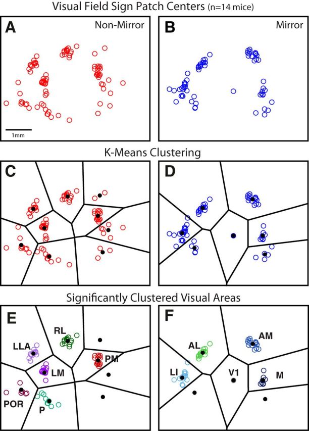
Classification of visual areas based on clustering of patch centers after alignment across animals. A, B, Scatter plot of mirror and nonmirror patch centers from each animal, after alignment of the maps across cases using the CoM of the largest patch (i.e., V1) and the direction of its horizontal gradient. Some patch centers fall into visible spatial clusters, whereas others appear more independent. C, D, Voronoi lines (black) illustrate boundaries between k-means clusters. Mean CoM of each cluster is shown as a black dot. E, F, Significant clusters remaining after shuffling analysis (see Materials and Methods). Patches from the more variable clusters were removed from further analysis. Also note that some significant clusters have fewer patches in E and F than in C and D. Patches in significant clusters were removed when there was a closer patch to the cluster's mean CoM, for the same animal. Remaining patch centers are considered reliably identified visual areas, found in a consistent spatial position across animals, labeled and color coded according to their grouping and anatomical position relative to V1. For the set of nonmirror image areas: LM, RL, PM, P, POR, and LLA. For the set of mirror image areas: V1, LI, AL, AM, and M. Tick marks represent 1 mm intervals in scale.

Quantifying scatter in areal position.

To quantify the variability in the position of each visual area, relative to area size (see Fig. 4E), we computed the following:

The numerator is the absolute distance between the visual area's CoM in a given animal and the mean CoM of the visual area across animals (millimeters). The average of the numerator across animals is independently plotted in Figure 4D. The denominator is the square root of the visual area's cortical coverage (square millimeters). The average cortical coverage is independently plotted in Figure 4C. The average of this ratio, across animals, is indicated by the brackets. This normalized measure for the scatter of each area is plotted in Figure 4E.

Figure 4.

Cortical coverage and variability in area position across animals. A, Overlay of all area boundaries across experiments, aligned using V1's CoM and horizontal gradient direction. Areal identity of patch borders was determined according to the classification procedure described in Figure 1. B, Combined scatter plot of visual area centers from all experiments, with each area's mean location in black. C, Average and SE of area size across subjects. D, Scatter in area position for each area. Scatter for each area is defined as the mean distance (mm) between the center locations (colored dots in B) and the average center (black dots in B). Scatter for V1 equals zero because V1's center was used to align all experiments. E, Scatter in area position normalized by area size provides an estimate of how consistently a given area can be found in the same cortical location across animals.

Coverage overlap.

Each pixel (i, j) of the image matrix in Figure 6G was computed as follows:

where D_i and D_j are the visual field coverage profiles (thresholded) from the visual area labeled on the x-axis and y-axis, respectively. D equals 1 where the coverage profile (see Fig. 6C) is >0.3, and it equals 0 otherwise. Coverage overlap values near 1 indicate that the coverage profile of the visual area on the y-axis is contained within the coverage profile of the visual area on the x-axis. Pixel values near 0 indicate that the two coverage profiles are largely exclusive.

Figure 6.

Visual coverage of higher areas is often incomplete or biased in space. A, Map of visual eccentricity computed from the average horizontal and vertical retinotopy across animals (Fig. 5). The origin was defined as the intersection of V1, LM, and RL, corresponding to the intersection between the horizontal and vertical meridians. Black lines indicate the computed area borders; white lines indicate iso-contours at 30° and 60°. B, Map of polar angle computed from the average vertical and horizontal retinotopy across animals (Fig. 5). A, B, Tick marks are 1 mm. C, Each panel represents the extent of the visual field covered by each area across cases, with iso-contour lines of eccentricity shown at 0°, 30°, and 90°. Color at each position is the proportion of experiments in which the given visual area showed coverage, limited to the experiments in which the area was found. The coverage profiles from the areas found in the average map (Fig. 5) are also shown as a black contour in each panel. Comparison of visual representations across areas demonstrates differences in the extent and region of visual coverage. D, Average total visual coverage for each identified region. V1 covers a large extent of the visual hemifield, whereas higher areas represent significantly smaller portions of space. E, CoM of visual field coverage profile for each area reveals biases in visual representations toward particular parts of space. F, Each bar represents the proportion of total coverage within each visual field quadrant of the polar coordinate system. Upper quadrants are above the 0° altitude line, and nasal quadrants are in the central 45° of visual space. G, Matrix of visual field overlap between each pair of areas. Coverage overlap was determined as the intersection of coverage, divided by the coverage of the area on the y-axis. Black dots indicate pairs of neighboring areas that have the same visual field sign and were nearby on the cortex.

Cortical magnification.

Magnification maps (see Fig. 7B) were computed using the inverse of the Jacobian determinant (mm²/deg²) at each pixel. Variables in the equation below are identical to those in Equation 4 as follows:

The principle axis of magnification at each cortical location (Fig. 7B) was computed using the gradients of horizontal and vertical retinotopy as follows:

Figure 7.

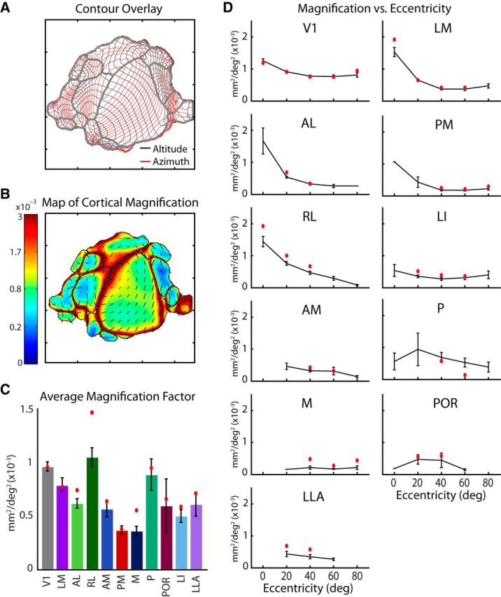
Differences in cortical magnification between areas and across visual eccentricity. A, Overlay of altitude and azimuth contours for the average map illustrating the relationships between vertical and horizontal gradients across cortical space. Contour lines are spaced at 5 degree intervals. B, Cortical magnification computed for each pixel of the average map (in mm²/deg²). An increase in magnification is observed at the lateral V1 border, at the intersection with LM and RL, corresponding to the center of visual space. A, B, Tick marks are 1 mm. C, Magnification averaged across all pixels for each area across cases, with the values for the average map in red. Although the majority of areas have lower magnification compared with V1, as would be expected from having smaller total cortical coverage, a few, notably RL, have similarly high magnification, perhaps associated with their incomplete coverage of visual space, or an emphasis on the nasal visual field. D, Relationship between magnification and visual eccentricity determined for each visual area across cases (black) and in the average map (red). A trend toward higher magnification at central representations is observed for several areas. However, others either lack coverage of the central visual field or show no trend.

Results

Automatic identification of visual areas from retinotopic maps

The goal of this study was to identify the spatial layout and boundaries of mouse visual cortical areas and characterize the visual field representation of each identified area. A visual area is defined as having a single orderly representation of space that can be consistently identified across individuals (Wandell et al., 2007). We designed an algorithm to identify regions that meet this definition by applying a series of automated processing steps to maps of visual topography (Table 1). The analyses all rely on retinotopic maps obtained with intrinsic signal imaging, representing the right visual hemifield in spherical coordinates (azimuth and altitude, which approximate curvilinear Cartesian coordinates near the center of gaze) (Marshel et al., 2011). Visual maps were segmented according to four specific criteria that quantify features of visuotopic organization and compute areal boundaries. The computational details of the algorithm are given in Materials and Methods. A general description of the rationale behind each step follows, with the results of a single experiment used as a guide (Fig. 1).

Table 1.

Summary of algorithm to identify borders of visual areas^a

Visual area criteria	Processing steps to impose criteria
(1) Area must have orthogonal retinotopy contours and consistent visual field sign	Thresholding of visual field sign map to create initial area borders (Fig. 1D)
(2) Area must have a nonredundant visual field representation within its borders	Compare “integral” versus “union” of visual coverage. Segment area with watershed if redundant (Fig. 1E)
(3) Adjacent areas with same visual field sign must have overlapping visual coverage	Compute overlap of all adjacent, same sign areas. Fuse adjacent areas if representation is nonoverlapping (Fig. 1F–J)
(4) Area must be at a consistent cortical location across experiments	“Significantly clustered” patches are identified as a visual area (Fig. 3)

^aLeft column is the list of four criteria that must be met to identify each patch as a visual area. Right column summarizes the processing steps taken to enforce the corresponding criterion.

The first criterion that a visual area must satisfy is having a consistent visual field sign within its borders (Sereno et al., 1994, 1995). At each cortical location, taking the sine of the angle between the gradients of vertical and horizontal retinotopy yields a map of visual field sign (Fig. 1A–C). The absolute value of this metric indicates the degree of orthogonality between the map gradients (magnitude of the difference between the two vectors), and the sign indicates whether the representation of visual space across the cortical surface is a reflection of the visual field (i.e., “flipped” along an arbitrary axis). Negative regions, such as the large blue patch in the middle of Figure 1C (i.e., V1), are mirror image transformations of the visual field. Positive regions, such as the smaller extrastriate patches in red surrounding V1, are nonmirror image transformations of the visual field. Transitions between positive and negative values in the map indicate the locations of reversals in the retinotopic gradients and provide a robust way to find borders between different visual field representations (Sereno et al., 1994; Warnking et al., 2002). Thresholding the map of visual field sign results in a set of discrete patches (Fig. 1D). For pairs of adjacent visual areas that are of the opposite field sign, the visual field sign analysis correctly delineates their borders. However, the possibility remains that two distinct visual field representations could have the same visual field sign and share a border, as is the case for some adjacent regions in humans (Larsson and Heeger, 2006; Wandell et al., 2007). The second criterion addresses this issue.

The second criterion a visual area must meet is that it cannot have a redundant representation of visual space. For instance, if a patch identified in the previous step contains multiple pixels that represent the same visual field location, this would indicate that it contains more than one visual area. To check each patch for redundancy, we compared the integral of visual field coverage over all pixels within a patch to the union of coverage by the patch (Eq. 4). Redundancy would yield an overestimate of coverage by the integral measure compared with the union, resulting from a duplication in the representation by multiple pixels. Figure 1E is a scatter plot comparing the integral to the union for the patches in Figure 1D. All patches sit along the unity line, with the exception of patch no. 11. Redundant patches, such as no. 11, were segmented automatically by applying the marker-controlled watershed algorithm to a map of visual eccentricity (Eq. 5). The watershed segmentation creates a border at the “ridge line“ that separates local minima in the visual eccentricity map. This method takes into account the relative size and rate of change of the map gradients to create accurate borders.

The third criterion requires that all adjacent areas of the same visual field sign have overlapping representations of visual space. This largely serves to check that the processing steps under Criterion 1 did not create inappropriate boundaries. For instance, if a single visual map were improperly split into separate patches, combining the two would produce a more complete, yet still nonredundant representation of space, satisfying our definition of a visual area. In turn, we merged each pair of neighboring same sign patches, assessed for redundancy as done for Criterion 2, and simply left them fused if their visual representations were nonoverlapping. Figure 1F shows the visual field coverage for pairs of neighboring patches that were split by the preceding steps of the algorithm. In the first three examples (Fig. 1F), despite being adjacent on the cortex with the same visual field sign, each pair has overlapping visual field coverage and was therefore appropriately segmented by the algorithm. In contrast, the final example in Figure 1F shows essentially no overlap, so the two patches were fused and considered as a single area.

The final set of boundaries (Fig. 1G–I) computed from the retinotopic maps in this experiment contains individual visual field maps fulfilling the first three requirements in our definition of a visual area. A clear correspondence between the computed borders and reversals in retinotopy can be observed in the contour plots of altitude and azimuth (Fig. 1G,H). Additional examples of retinotopic maps and the associated visual field sign maps and borders are shown in Figure 2. Upon visual inspection, some patches are consistently identified at the same relative cortical location in all experiments. However, others, particularly those along the posterior edge of the visual cortex, display more variability across cases.

Figure 2.

Topography and patch boundaries for individual examples. Each row corresponds to an individual mouse. A, Visual field sign maps computed from vertical and horizontal retinotopy for each case. B, Horizontal retinotopy, shown as azimuth contours, with values indicated by the associated color map. Patch boundaries identified by the segmentation algorithm are overlaid in black. C, Vertical retinotopy, shown as altitude contours, with corresponding color map. Patch boundaries identified by the segmentation algorithm are overlaid in black. D, Borders identified by the segmentation algorithm with the CoM for each patch indicated as blue points for mirror image transformations and red points for nonmirror image representations. Scale is indicated by tick marks, with distance between ticks = 1 mm.

The fourth and final criterion is that a visual area must be reliably identified at the same location in different individuals. Whereas the preceding steps compute borders for each independent experiment, the final step looks across experiments to determine whether the identified patches have a statistically significant mean location. The position of the visual cortex within the camera's field of view for each experiment was variable, so the maps were aligned using an easily identified landmark: the largest, most reliably identified central patch, corresponding to V1. The map from each experiment was first shifted to align V1's CoM and then rotated to align the mean direction of V1's horizontal retinotopic gradient. Following this alignment, we overlaid the CoMs of all patches in the 14 experiments, shown separately for mirror and nonmirror image representations in Figure 3A, B. At first glance, there is visible structure in the arrangement of the patch centers. To evaluate whether patch centers fell into clusters that could be associated with particular visual areas, k-means clustering was performed on the mirror and nonmirror scatter plots (see Materials and Methods). The Voronoi lines in black segregate each identified cluster, along with a black dot for each cluster mean (Fig. 3C,D). As our definition of a visual area states that regions should be reliably identified across individuals, we performed an additional analysis to remove patch centers that were not associated with significant clusters. A shuffling analysis (see Materials and Methods) identified 11 consistently separated clusters of patch centers, shown in Figure 3 E, F. Patch centers that did not belong to significant clusters were excluded from further analysis. Furthermore, some clusters had multiple patches from the same animal. In these cases, only the patch closest to the cluster's mean CoM was used for further analysis.

The spatial arrangement of the clusters closely matched previous descriptions of the layout of visual areas in the mouse. Nine of the definitively classified visual areas corresponded to previously described visual areas: V1, LM, LI, AL, RL, AM, PM, P, and POR (Olavarria et al., 1982; Olavarria and Montero, 1989; Wang and Burkhalter, 2007). In addition, we were surprised to find two clusters of patch centers that did not map on to any known mouse visual areas. Although unexpected, these two regions met all conditions of our analysis and were robustly identified across cases (Fig. 3E,F), warranting their classification as independent, well-defined visual areas. The first belonged to the set of nonmirror patches and was located on the far lateral side of the visual cortex, neighboring to area AL. The second unexpected cluster belonged to the set of mirror image patches and was located medial to V1 and just posterior to area PM. Although not previously reported in mice, visual regions in corresponding locations have been described in other rodents, including the rat, and we labeled these analogous regions accordingly as the LLA and M visual areas (Olavarria and Montero, 1984; Malach, 1989; Sereno and Allman, 1991; Spatz et al., 1991; Espinoza et al., 1992). In contrast, another area predicted by anatomy to be located anterior to V1, between RL and AM, the anterior area, A (Wang and Burkhalter, 2007), was not reliably detected by our analysis procedure, although a small patch in this region was observed in 2 of 15 cases (Fig. 3C, top right cluster). However, the field sign of this patch was the opposite of that predicted for A based on topograpy of corticocortical projections (compare Fig. 1D, patch 13 with Wang and Burkhalter, 2007).

Several more variable patch centers were observed at the posterior edge of the cortex, on both the medial and lateral sides of V1. A small mirror image patch was sometimes detected between P and POR (Figs. 2 and 3), potentially corresponding to area PL defined in previous studies (Olavarria and Montero, 1989). However, the cluster associated with this patch was not deemed significant in the shuffling analysis and was not included in further analysis. An additional nonmirror image patch was sometimes observed just lateral to LI (Figs. 1, 2, and 3), potentially corresponding to area LL (Olavarria and Montero, 1984; Malach, 1989; Sereno and Allman, 1991), but again was not consistently delineated. On the medial side of the visual cortex, in the area cytoarchitecturally defined as V2MM (Wang and Burkhalter, 2007; Paxinos and Franklin, 2004), visual responses were often evident but did not show consistent topography. As a result, visual field patches of both mirror and nonmirror image field sign were sometimes detected in the region proximal to AM, PM, and M (Figs. 2 and 3), but these were variable and consequently not classified as visual areas according to our analysis. A region bordering area M along the cortical midline, in the anatomical location corresponding to the retrosplenial cortex, was observed as being visually mapped in some cases. However, only a portion of the known extent of this area was typically visible within the field of view, resulting in partial maps that were not reliable across animals.

It is important to note that the classification of visual areas reported here is subject to the limitations of our experimental approach (e.g., the limited resolution of intrinsic imaging and/or the use of a simple visual stimulus of a defined size and speed) and is specific to our definition of a visual area. Further studies using other methods will verify the relationship between the area boundaries defined here and additional functional and anatomical descriptions of cortical visual areas.

Uncertainty in the position of visual areas

Although the arrangement of visual areas was fairly stereotyped across animals, evident from the overlay of area borders (Fig. 4A) and the overlay of CoMs after alignment (Fig. 4B), the relative location of different higher visual areas had varying degrees of consistency. Quantifying an extrastriate area's positional uncertainty across multiple animals can be an important guide for their targeting in future experiments. Because V1 is the most reliably and clearly identified area, with intrinsic imaging as well as other localization methods, a measurement of variability within this reference frame serves as an informative baseline. As described above, the maps from each experiment were independently shifted and rotated to align V1 for subsequent analysis.

To measure the positional uncertainty for each visual area, we first quantified each area's size (Fig. 4C) along with the scatter of the CoMs across subjects (Fig. 4D). Higher visual areas were all significantly smaller than V1 (4.04 mm²), with the next largest area being LM (1.01 mm²), followed by RL (0.92 mm²), and all other areas falling between 0.13 and 0.42 mm² (Fig. 4C). The CoMs of the extrastriate visual areas had different degrees of scatter: the average cortical distance from the mean CoM of all areas fell between 0.09 and 0.22 mm, with LM and AL having the lowest (0.094 mm, 0.095 mm), and P and POR having the highest (0.22 mm, 0.19 mm) (Fig. 4D). The values from Figure 4C, D were combined to compute the ratio of scatter to the square-root of area size, shown in Figure 4E. This normalized metric more directly indicates the ability to accurately identify the position of extrastriate areas relative to V1. For instance, one of the larger cortical areas with relatively low variability, LM, shows a distribution of area centers that is only 9% of the size of the entire area, meaning that it could be reasonably targeted using prior knowledge of the position of V1 alone. In contrast, the positional scatter of POR is 62% of its overall size, making it difficult to identify accurately without a direct measurement of POR's borders in a given individual. These differences are important to consider when targeting specific higher visual areas using localization methods that rely on generalized coordinates or frames of reference, as well as when interpreting results of studies that are highly dependent on area identification.

Average retinotopic organization of visual cortex

To further assess the architecture of mouse visual cortex, we computed the average horizontal and vertical retinotopic map after alignment (Fig. 5). Specifically, the average map of vertical retinotopy was taken to be $\measuredangle {{\displaystyle {\sum }_{a}M}}_a{e}^{i{V}_a}$, where M_a is the aligned map of response magnitude (i.e., the F1 amplitude) and V_a is the aligned map of vertical retinotopy, for animal a. To define area borders in the average map, we used the segmentation algorithm based on the map of visual field sign (Fig. 5A) as before (Criteria 1–3).

Figure 5.

Average topographic maps demonstrate features of mouse visual cortical organization. A, Visual field sign map produced by a weighted average of retinotopic maps from all experiments, emphasizing those with stronger responses. The segmentation algorithm was used to identify area boundaries based on retinotopic gradients, as with individual cases. Areal organization of the average map closely corresponds to the layout observed in individual cases, with all major areas identified. B, Average azimuth contours, in degrees, showing progression of the horizontal gradient from temporal fields in red to the nasal field in blue. Area boundaries are shown in black. C, Average altitude contours, in degrees, showing progression of vertical retinotopy from the lower fields in blue to the upper field in red. Area boundaries are in black.

In the map of horizontal retinotopy, shown as azimuth contours in Figure 5B, the vertical meridian occurs at the nasal most representation in the map of horizontal retinotopy (∼−50° azimuth, blue) and is the most prominent feature separating V1 from lateral extrastriate areas. The progression of visual space in areas LM, AL, RL, and P going from medial to lateral and away from V1 moves from the nasal visual field, out to temporal. Areas LI and POR share the lateral and posterior borders of LM and have a reflection of this topography across their borders, reversing from temporal to nasal as they move away from LM toward the lateral and posterior edges of the brain. In contrast, the map of horizontal retinotopy in area P shares LM's organization, appearing almost continuous along V1's posterior edge. The horizontal map in area LLA is a reflection of that of LI along the anterior–posterior axis, with nasal visual field represented more posteriorly and the temporal fields at its most anterior point. RL is medial to AL and LLA, along V1's rostral edge, and also moves from nasal to temporal as it reflects away from V1. However, the visual maps observed in RL are often complex and sometimes show a warping of visual space in the center of the area, creating a ring-like structure and resulting distortion in visual field sign. This feature may correspond to the observed pattern of callosal connections in this region (Olavarria and Montero, 1989; Wang and Burkhalter, 2007; Wang et al., 2011). Finally, areas AM, PM, and M are contained within a long strip of cortex on the medial edge of V1. The maps of horizontal retinotopy in AM and PM are reflections of each other, with the vertical meridian running along the border between them. The map in M is a reversal of that in V1, moving from temporal to nasal as it extends medially.

In the map of vertical retinotopy (Fig. 5C), the horizontal meridian (0° altitude, green) typically runs through the middle of visual areas, with peripheral representations corresponding to the boundaries between distinct visual field maps. The horizontal meridian extending through the middle of V1 diverges at the LM-AL-RL border, splitting into three separate arms, one running through each area. LM's horizontal meridian extends laterally into LI, then curls around toward the posterior edge of the cortex through POR and P. The upper visual field is represented by the caudal portion of V1 and along the boundary between LM, LI, P, and POR. Although the most posterior edge of the cortex can be difficult to image, a transition toward lower field representations is typically observed at the caudal boundary of P and POR. A reversal in the vertical gradients at the lower visual field marks the intersection between LM, LI, AL, and LLA. Moving more anterior, AL and LLA are bounded by a reversal at the upper fields, transitioning into RL. The vertical gradients of medial areas AM, PM, and M are aligned with the horizontal meridian running through the center of all three areas, moving toward the lower fields as they approach V1.

Characterizing visual field coverage

The region of visual space covered by a cortical area has important implications for its overall function. For instance, ventral stream areas in primates primarily represent the central visual field, enhancing processing of object features near the fovea, whereas parietal visual areas tend to over-represent the periphery and process spatial relationships (for review, see Gattass et al., 2005). Our measurements show that mouse extrastriate visual areas have consistent biases in visual field coverage as well.

To measure the average visual field coverage by a given cortical area, offline steps were taken to ensure that the stimulated eye of all subjects was registered to a common point of visual space. Although efforts were made during the experiment to have the visual stimulus at the same location in all subjects, small differences in head and/or eye alignment were nonetheless evident in the retinotopic maps. To correct for these differences, we registered the maps with an easily identified anatomical location: the intersection of areas V1, LM, and RL. That is, the [0 0] point of altitude and azimuth was shifted to the V1-LM-RL point of intersection. In addition to being easily defined anatomically, this point is a natural reference for assessing visual coverage, as it coincides with the intersection of the vertical and horizontal meridians at the center of visual space. Although the central visual field corresponds to the center of the retina in primates, this is not the case in species with lateral facing eyes. In mice, the center of gaze lies 60 degrees lateral to the midline, whereas the central visual field (directly in front of the animal) and region of binocular overlap are mapped onto the temporal retina (Oommen and Stahl, 2008; Sterratt et al., 2013). Accordingly, shifting the origin of the maps to this location on the brain produces maps of visual eccentricity (Fig. 6A) and polar angle (Fig. 6B).

Each panel of Figure 6C shows the visual field coverage by the designated visual area in this shifted coordinate space. The cardinal axes are altitude and azimuth coordinates, and contours illustrate iso-eccentricity lines at 30° intervals. The vertical meridian (nasal-most representation, or central visual field) is at 0° azimuth, and the horizontal meridian (midline separating upper from lower fields) is at 0° altitude. Black regions indicate points in visual space that were represented every time the area was found, whereas white regions were never represented by the area. This depiction is considered the “coverage profile” for each area and demonstrates the reliability of having coverage at each receptive field location across animals. The black contour overlaid on each plot represents the coverage profile outline obtained from the area in the average map (Fig. 5).

Comparison of coverage profiles between visual areas presents several interesting observations. First, it is apparent that the region of space covered by V1 is significantly larger than that of all other visual areas, indicating that higher areas typically have less than complete representations of space. The average visual field coverage (deg²) is shown in Figure 6D, with PM, LM, and RL having the next highest degrees of coverage, after V1. The second distinction is that many higher visual areas show a significant bias in the region of space they represent. Whereas V1's coverage profile is centered near the midpoint of the mouse's eye (∼0° altitude, ∼50° azimuth), the coverage profiles of higher areas are skewed away from this point. For example, RL's representation of space is clearly biased toward the lower nasal visual field, below the horizontal meridian (0° altitude) and toward the vertical meridian (0° azimuth). In contrast, PM preferentially represents the temporal visual field, and area P primarily covers the upper visual field. LM's coverage profile is the closest in appearance to that of V1, although it still has a significantly reduced representation. These biases are summarized in Figure 6E, which plots the CoM of each area's coverage profile. Figure 6F is also a summary of the biases in coverage, showing the proportion of each area's coverage profile within four different quadrants of polar coordinates.

Finally, we characterized the degree of coverage overlap between all pairs of areas, shown as a matrix in Figure 6G. The value for each position in the matrix was computed from the sum of the coverage profiles from the visual areas on the x- and y-axes, normalized by the profile of the area on the y-axis (see Materials and Methods). Consequently, pixel values near one (red) indicate that the coverage profile of the visual area on the y-axis is contained within the coverage profile of the area on the x-axis. Pixel values near zero (blue) represent coverage profiles that are largely exclusive. Pixels with a black dot indicate pairs of areas that are neighboring and have the same visual field sign.

Cortical magnification in each visual area

The cortical magnification factor is the amount of cortical territory devoted to processing a given unit of visual space. The overlay of altitude and azimuth gradients from the average map can be used to illustrate these relationships (Fig. 7A). The contour lines for both gradients are equally spaced at 5 degree intervals, meaning that each square created by their intersection corresponds to a 25 deg² region of visual space. The cortical area (mm²) within each 25 deg² region is proportional to the magnification factor (mm²/deg²) at that cortical location. Cortical magnification is also represented by the color map in Figure 7B. The colors represent the Jacobian determinant computed at each pixel from the maps of retinotopy (Eq. 9). We quantified each area's average magnification factor by taking the average value across all pixels within each of the visual area boundaries of the map in Figure 7B. These mean values are indicated by red dots in the plot of average magnification across experiments in Figure 7C. We also performed the same analysis on each of the 14 individual experiments to determine the average areal magnification across cases, represented in Figure 7C. A logical expectation would be that magnification was proportional to visual area size. For instance, area PM has the lowest average magnification, in accordance with it being a small area with a relatively larger coverage profile. However, this trend did not generalize across areas because of the variability in visual field coverage. For instance, RL has a higher mean magnification factor than V1, a result of its emphasis on the nasal visual field. The limited visual field representation of many smaller areas also creates a much higher magnification than what might be expected based on V1's magnification.

From the map in Figure 7B, it appears that magnification factor is not constant across each area's representation of the visual field, as may otherwise be expected by the relatively homogeneous density of photoreceptors in the mouse retina (Dräger and Olsen, 1981; Jeon et al., 1998). Instead, an increase in magnification can be seen at the V1-LM-RL intersection, which corresponds to the binocular zone and the center of visual space. To directly examine the relationship between magnification factor and eccentricity, we computed the mean magnification within 20° intervals of eccentricity. The black curves in Figure 7D show the average magnification across experiments, within each eccentricity interval. The red dots are from the average map alone (Fig. 7B). For the largest areas (V1, LM, RL, PM, and AL), there is an increase in magnification at 0 degrees eccentricity, which is likely accounted for by the binocularity at this location. Greater magnification at the binocular zones of the cortex is to be expected, as these regions likely receive more inputs per degree of visual field. For areas, such as LI, ALL, and M, no relationship is observed. However, for the two posterior lateral areas, P and POR, an interesting trend occurs where magnification is increased in the middle range of eccentricities, but not at the center of space or extreme periphery.

Cortical magnification is not necessarily an isotropic quantity, meaning that the visual field representation may be stretched along a particular direction of the cortex. This is clearly the case for many of the areas in the mouse. The regions enclosed by the contour intersections (Fig. 7A) are not perfect squares but are often elongated. This corresponds to the principal axis of magnification and can be quantified at each pixel using the Jacobian matrix from the retinotopic maps (see Materials and Methods). The black lines overlaid on the map of Figure 7B represent the principal axes of magnification sampled every 250 μm. For the map of V1, it appears that the elongation occurs parallel to the altitude gradient, indicating an expanded representation along the vertical dimension of visual space.

Discussion

Identifying visual cortical areas

This investigation builds on previous work by providing a quantitative method for parceling visual areas based on their visuotopic organization. Intrinsic signal imaging is a valuable tool for studies that aim to correlate visual area identification with function, behavior, and anatomy: it is minimally invasive, reliable, and yields a field of view with sufficient width and resolution to capture the majority of topographic compartments of the mouse visual cortex. Although a few studies have targeted recordings to higher areas using retinotopic mapping with intrinsic signal imaging (Andermann et al., 2011; Marshel et al., 2011; Glickfeld et al., 2013; Tohmi et al., 2014), none has quantitatively determined the borders between areas. Interpreting areal organization from retinotopy is especially challenging in the mouse where maps can be small, clustered, or distorted, emphasizing the need for a rigorous, unbiased method. Our experimental and analytical approach allowed us to resolve the layout and variability of 11 visuotopically defined areas, two of which had not been previously identified in the mouse.

We were surprised to find a visuotopic map just lateral to area AL that was not previously identified based on projections from V1 (Olavarria and Montero, 1989; Wang and Burkhalter, 2007). A region in the corresponding location has been described in rats as area LLA, and we have named this patch accordingly (Olavarria et al., 1982; Olavarria and Montero, 1984; Thomas and Espinoza, 1987; Malach, 1989). Given its proximity to auditory cortex, it is possible that LLA is involved in audiovisual integration and may correspond to area DP (Wang et al., 2011, 2012). The lack of direct input from V1 to LLA (Wang and Burkhalter, 2007) indicates that this area may be relatively higher in the visual system hierarchy and may receive its primary input from other extrastriate regions. The retinotopic structure of area LLA was present in some previous map descriptions in the mouse but was not identified as a distinct area, presumably because of the difficulty in identifying reversals and borders subjectively (Marshel et al., 2011). Our algorithm reliably identified this region in nearly every case, demonstrating the utility and necessity of more quantitative, automated approaches.

We found another unexpected reversal in visual field sign just posterior to PM, revealing an additional visuotopic map for area M. The border between M and PM may have been difficult to detect in previous studies because of the subtle changes in the scale and direction of the retinotopic gradients at this location. However, area M and its borders are revealed by visual field sign analysis across cases (Fig. 3) and in the average map (Fig. 5). Although this region has not been shown to receive topographic input from V1 in the mouse (Wang and Burkhalter, 2007), it is a projection target of V1 and lateral extrastriate cortex in the rat (Olavarria and Montero, 1984; Malach, 1989).

Area A, proposed to be just anterior to V1, between RL and AM, was not readily evident in the visual field sign maps obtained in this study. A likely explanation for this discrepancy is that area A does not have a clear retinotopic structure, consistent with the degree of overlap in topographic projections from V1 (Wang and Burkhalter, 2007). It is also possible that A integrates information from multiple sensory modalities, evidenced by its position in the posterior parietal cortex, or that stimulus parameters, including stimulus size and/or speed, were not matched to the preferences of this area.

Lateral–temporal areas LI, P, and POR are small and had more positional variability than most other areas. This may be partially accounted for by the difficulty of detecting such a tight cluster of areal borders with intrinsic imaging or indicate that these regions have more complex feature dependencies, large receptive field sizes, or coarser visuotopic organization. Nonetheless, area LI was evident in every case. Posterior to LM and LI, we observed several small visuotopic maps of alternating field sign, consistent with previous studies demonstrating multiple distinct projection fields of V1 in this region (Olavarria and Montero, 1981, 1989; Olavarria et al., 1982; Montero, 1993; Wang and Burkhalter, 2007). We observed an additional visuotopic map lateral to P and LI in a location corresponding to the postrhinal area, POR (Burwell and Amaral, 1998; Burwell, 2001; Wang and Burkhalter, 2007). This region was at the extreme posterior lateral edge of our field of view and may not have been fully visible in all animals, making it likely that its representation has been underestimated (Burwell, 2001). In a few cases, we found additional visuotopic maps lateral to LI and POR, potentially corresponding to areas 36p or TEp as described by Wang et al. (2012).

The ability to detect visual field representations of nearly a dozen higher visual areas using a simple drifting bar stimulus is highly beneficial for mapping and localization studies, and the methods described here should prove useful for areal identification. However, it is likely that many extrastriate regions have more complex receptive field properties and are more effectively driven under natural conditions. Furthermore, higher-order areas may require multimodal input and have representations that are increasingly dependent on behavioral state and context. Experiments taking advantage of richer stimuli and higher resolution imaging methods in awake animals will be essential to provide a more detailed view of functional representations in extrastriate cortex.

Representations of visual space in extrastriate areas

We found that mouse extrastriate visual areas consistently lacked a full representation of the visual field and overrepresented particular regions of space. The representational bias of a given visual area was typically correlated with the region mapped onto the neighboring portion of V1. Lateral areas primarily emphasized the central visual field, whereas medial areas were biased toward the periphery. Incomplete and biased representations of space have also been observed in extrastriate areas of primates (Baizer et al., 1991; Gattass et al., 2005; Orban, 2008). However, such coverage biases appear more extreme in mice, which may be driven by the need for functionally specific encoding of localized regions of the visual field on a smaller cortex. For example, RL devotes a relatively large portion of its cortical territory to the lower nasal visual field, implying that behaviors depending on this area require detailed information from this region of space. A potential role for RL is the combined coordination of vision and whisking (Olcese et al., 2013), consistent with the fact that the nasal visual field coincides with the location of whisker stimuli. Additional support for RL's role in multimodal integration is its physical proximity to somatosensory cortex and associated connectivity (Wang and Burkhalter, 2007; Wang et al., 2012). We may find similar clues in determining the behavioral roles of other extrastriate areas.

It is likely that the absolute extents of the visual field representations we have observed are artificially reduced by the limited resolution of intrinsic signal imaging (blurring of the retinotopic maps could clip the visual field representations around their edges) or other experimental conditions. For instance, our measurement of V1's visual coverage is ∼100° in azimuth and 60° of altitude (Fig. 6), whereas an electrode study using a spherical display measured these to be 140° and 100°, respectively (Wagor et al., 1980). We would predict similar discrepancies for the higher visual areas. However, it is unlikely that this would significantly alter our conclusions about relative biases in coverage between areas.

Higher cortical magnification near the central visual field

Changes in magnification factor reflect a visual area's division of labor across the visual field. In general, if a particular subregion within a visual area receives more inputs per degree of visual field, then it will require more neurons to encode the extra information. Consistent with previous reports (Wagor et al., 1980; Schuett et al., 2002), we observed an increase in magnification at the representation of the nasal visual field of V1, in the region of the binocular zone. Furthermore, we showed that extrastriate areas with coverage of the central visual field also showed a similar increase in magnification (LM, AL, RL, and PM). In addition to binocular inputs, a recently observed sampling bias in the retina may also contribute to the higher cortical magnification in the central visual field. A specific subpopulation of Alpha-On RGCs, thought to subserve higher resolution vision, displays an increased density at the temporal retina (Bleckert et al., 2014). It is possible that this region shares functional similarities with the foveal representation of other species. Further investigation into the relationships between cortical representations and retinal specializations may yield additional insights (Picanço-Diniz et al., 2011; Chang et al., 2013; Scholl et al., 2013; Wallace et al., 2013).

In conclusion, a hallmark of sensory cortex is the grouping of neurons with similar function, particularly through selective inputs from parallel pathways. This architecture allows for a powerful experimental paradigm, whereby the locations of functional compartments are first identified noninvasively, followed by targeted injections or recordings for subsequent manipulation or characterization. We show that retinotopic mapping with intrinsic signal imaging combined with objective analytical tools provides a means for targeting mouse visual areas, even when they are too small or too variable in their location to be targeted by approaches such as stereotaxic coordinates. Furthermore, rodent visual areas contain significant biases in both response properties (Andermann et al., 2011; Marshel et al., 2011; Tohmi et al., 2014) and visual field coverage (this study). This functional specialization is likely to be governed by parallel circuits (Glickfeld et al., 2013) and serve to guide adaptive behaviors. There is great promise in establishing a link between circuits and behavior by exploiting both the architecture of mouse visual cortex and genetic tools. Our objective, quantitative approach to characterizing the layout of mouse visual areas is an important element of this approach.

References

- Andermann ML, Kerlin AM, Roumis DK, Glickfeld LL, Reid RC. Functional specialization of mouse higher visual cortical areas. Neuron. 2011;72:1025–1039. doi: 10.1016/j.neuron.2011.11.013. [DOI] [PMC free article] [PubMed] [Google Scholar]
- Baizer JS, Ungerleider LG, Desimone R. Organization of visual inputs to the inferior temporal and posterior parietal cortex in macaques. J Neurosci. 1991;11:168–190. doi: 10.1523/JNEUROSCI.11-01-00168.1991. [DOI] [PMC free article] [PubMed] [Google Scholar]
- Bleckert A, Schwartz GW, Turner MH, Rieke F, Wong RO. Visual space is represented by nonmatching topographies of distinct mouse retinal ganglion cell types. Curr Biol. 2014;24:310–315. doi: 10.1016/j.cub.2013.12.020. [DOI] [PMC free article] [PubMed] [Google Scholar]
- Burwell R, Amaral D. Cortical afferents of the perirhinal, postrhinal, and entorhinal cortices of the rat. J Comp Neurol. 1998;205:179–205. doi: 10.1002/(sici)1096-9861(19980824)398:2<179::aid-cne3>3.0.co;2-y. [DOI] [PubMed] [Google Scholar]
- Burwell RD. Borders and cytoarchitecture of the perirhinal and postrhinal cortices in the rat. J Comp Neurol. 2001;437:17–41. doi: 10.1002/cne.1267. [DOI] [PubMed] [Google Scholar]
- Chang L, Breuninger T, Euler T. Chromatic coding from cone-type unselective circuits in the mouse retina. Neuron. 2013;77:559–571. doi: 10.1016/j.neuron.2012.12.012. [DOI] [PubMed] [Google Scholar]
- Dräger UC. Receptive fields of single cells and topography in mouse visual cortex. J Comp Neurol. 1975;160:269–290. doi: 10.1002/cne.901600302. [DOI] [PubMed] [Google Scholar]
- Dräger UC, Olsen JF. Ganglion cell distribution in the retina of the mouse. Invest Ophthalmol Vis Sci. 1981;20:285–293. [PubMed] [Google Scholar]
- Dumoulin SO, Hoge RD, Baker CL, Jr, Hess RF, Achtman RL, Evans AC. Automatic volumetric segmentation of human visual retinotopic cortex. Neuroimage. 2003;18:576–587. doi: 10.1016/S1053-8119(02)00058-7. [DOI] [PubMed] [Google Scholar]
- Espinoza SG, Subiabre JE, Thomas HC. Retinotopic organization of striate and extrastriate visual cortex in the golden hamster (Mesocricetus auratus) Biol Res. 1992;25:101–107. [PubMed] [Google Scholar]
- Gattass R, Nascimento-Silva S, Soares JG, Lima B, Jansen AK, Diogo AC, Farias MF, Botelho MM, Mariani OS, Azzi J, Fiorani M. Cortical visual areas in monkeys: location, topography, connections, columns, plasticity and cortical dynamics. Philos Trans R Soc Lond B Biol Sci. 2005;360:709–731. doi: 10.1098/rstb.2005.1629. [DOI] [PMC free article] [PubMed] [Google Scholar]
- Glickfeld LL, Andermann ML, Bonin V, Reid RC. Cortico-cortical projections in mouse visual cortex are functionally target specific. Nat Neurosci. 2013;16:219–226. doi: 10.1038/nn.3300. [DOI] [PMC free article] [PubMed] [Google Scholar]
- Hamdi MA. Modified algorithm marker-controlled watershed transform for image segmentation based on curvelet threshold. Middle-East J Sci Res. 2014;20:323–327. [Google Scholar]
- Huberman AD, Niell CM. What can mice tell us about how vision works? Trends Neurosci. 2011;34:464–473. doi: 10.1016/j.tins.2011.07.002. [DOI] [PMC free article] [PubMed] [Google Scholar]
- Jeon CJ, Strettoi E, Masland RH. The major cell populations of the mouse retina. J Neurosci. 1998;18:8936–8946. doi: 10.1523/JNEUROSCI.18-21-08936.1998. [DOI] [PMC free article] [PubMed] [Google Scholar]
- Kalatsky VA, Stryker MP. New paradigm for optical imaging: temporally encoded maps of intrinsic signal. Neuron. 2003;38:529–545. doi: 10.1016/S0896-6273(03)00286-1. [DOI] [PubMed] [Google Scholar]
- Lam L, Lee SW, Suen CY. Thinning methodologies: a comprehensive survey. IEEE Trans Pattern Anal Machine Intel. 1992;14:869–885. [Google Scholar]
- Larsson J, Heeger DJ. Two retinotopic visual areas in human lateral occipital cortex. J Neurosci. 2006;26:13128–13142. doi: 10.1523/JNEUROSCI.1657-06.2006. [DOI] [PMC free article] [PubMed] [Google Scholar]
- Luo L, Callaway EM, Svoboda K. Genetic dissection of neural circuits. Neuron. 2008;57:634–660. doi: 10.1016/j.neuron.2008.01.002. [DOI] [PMC free article] [PubMed] [Google Scholar]
- Madisen L, Zwingman TA, Sunkin SM, Oh SW, Zariwala HA, Gu H, Ng LL, Palmiter RD, Hawrylycz MJ, Jones AR, Lein ES, Zeng H. A robust and high-throughput Cre reporting and characterization system for the whole mouse brain. Nat Neurosci. 2010;13:133–140. doi: 10.1038/nn.2467. [DOI] [PMC free article] [PubMed] [Google Scholar]
- Malach R. Patterns of connections in rat visual cortex. J Neurosci. 1989;9:3741–3752. doi: 10.1523/JNEUROSCI.09-11-03741.1989. [DOI] [PMC free article] [PubMed] [Google Scholar]
- Marshel JH, Garrett ME, Nauhaus I, Callaway EM. Functional specialization of seven mouse visual cortical areas. Neuron. 2011;72:1040–1054. doi: 10.1016/j.neuron.2011.12.004. [DOI] [PMC free article] [PubMed] [Google Scholar]
- Montero VM. Retinotopy of cortical connections between the striate cortex and extrastriate visual areas in the rat. Exp Brain Res. 1993;94:1–15. doi: 10.1007/BF00230466. [DOI] [PubMed] [Google Scholar]
- Nauhaus I, Ringach DL. Precise alignment of micromachined electrode arrays with V1 functional maps. J Neurophysiol. 2007;97:3781–3789. doi: 10.1152/jn.00120.2007. [DOI] [PubMed] [Google Scholar]
- Olavarria J, Montero VM. Reciprocal connections between the striate cortex and extrastriate cortical visual areas in the rat. Brain Res. 1981;217:358–363. doi: 10.1016/0006-8993(81)90011-1. [DOI] [PubMed] [Google Scholar]
- Olavarria J, Montero VM. Relation of callosal and striate-extrastriate cortical connections in the rat: morphological definition of extrastriate visual areas. Exp Brain Res. 1984;54:240–252. doi: 10.1007/BF00236223. [DOI] [PubMed] [Google Scholar]
- Olavarria J, Montero VM. Organization of visual cortex in the mouse revealed by correlating callosal and striate-extrastriate connections. Vis Neurosci. 1989;3:59–69. doi: 10.1017/S0952523800012517. [DOI] [PubMed] [Google Scholar]
- Olavarria J, Mignano LR, Van Sluyters RC. Pattern of extrastriate visual areas connecting with striate cortex in the mouse. Exp Neurol. 1982;78:775–779. doi: 10.1016/0014-4886(82)90090-5. [DOI] [PubMed] [Google Scholar]
- Olcese U, Iurilli G, Medini P. Cellular and synaptic architecture of multisensory integration in the mouse neocortex. Neuron. 2013;79:579–593. doi: 10.1016/j.neuron.2013.06.010. [DOI] [PubMed] [Google Scholar]
- Oommen BS, Stahl JS. Eye orientation during static tilts and its relationship to spontaneous head pitch in the laboratory mouse. Brain Res. 2008;1193:57–66. doi: 10.1016/j.brainres.2007.11.053. [DOI] [PMC free article] [PubMed] [Google Scholar]
- Orban GA. Higher order visual processing in Macaque extrastriate cortex. Physiol Rev. 2008;88:59–89. doi: 10.1152/physrev.00008.2007. [DOI] [PubMed] [Google Scholar]
- Paxinos G, Franklin KB. The mouse brain in stereotaxic coordinates. New York: Elsivier; 2004. [Google Scholar]
- Pisauro MA, Dhruv NT, Carandini M, Benucci A. Fast hemodynamic responses in the visual cortex of the awake mouse. J Neurosci. 2013;33:18343–18351. doi: 10.1523/JNEUROSCI.2130-13.2013. [DOI] [PMC free article] [PubMed] [Google Scholar]
- Picanço-Diniz C, Rocha E, Silveira LC, Elston G, Oswaldo-Cruz E. Cortical representation of the horizon in V1 and peripheral scaling in mammals with lateral eyes. Psychol Neurosci. 2011;4:19–27. doi: 10.3922/j.psns.2011.1.004. [DOI] [Google Scholar]
- Polack PO, Contreras D. Long-range parallel processing and local recurrent activity in the visual cortex of the mouse. J Neurosci. 2012;32:11120–11131. doi: 10.1523/JNEUROSCI.6304-11.2012. [DOI] [PMC free article] [PubMed] [Google Scholar]
- Rosa MG, Tweedale R. Brain maps, great and small: lessons from comparative studies of primate visual cortical organization. Philos Trans R Soc Lond B Biol Sci. 2005;360:665–691. doi: 10.1098/rstb.2005.1626. [DOI] [PMC free article] [PubMed] [Google Scholar]
- Roth MM, Helmchen F, Kampa BM. Distinct functional properties of primary and posteromedial visual area of mouse neocortex. J Neurosci. 2012;32:9716–9726. doi: 10.1523/JNEUROSCI.0110-12.2012. [DOI] [PMC free article] [PubMed] [Google Scholar]
- Sato TK, Häusser M, Carandini M. Distal connectivity causes summation and division across mouse visual cortex. Nat Neurosci. 2014;17:30–32. doi: 10.1038/nn.3585. [DOI] [PMC free article] [PubMed] [Google Scholar]
- Scholl B, Burge J, Priebe NJ. Binocular integration and disparity selectivity in mouse primary visual cortex. J Neurophysiol. 2013;109:3013–3024. doi: 10.1152/jn.01021.2012. [DOI] [PMC free article] [PubMed] [Google Scholar]
- Schuett S, Bonhoeffer T, Hübener M. Mapping retinotopic structure in mouse visual cortex with optical imaging. J Neurosci. 2002;22:6549–6559. doi: 10.1523/JNEUROSCI.22-15-06549.2002. [DOI] [PMC free article] [PubMed] [Google Scholar]
- Sereno MI, Allman JM. Cronly-Dillon J, Leventhal A, editors. Cortical visual areas in mammals. The neural basis of visual function. 1991:160–172. [Google Scholar]
- Sereno MI, McDonald CT, Allman JM. Analysis of retinotopic maps in extrastriate cortex. Cereb Cortex. 1994;4:601–620. doi: 10.1093/cercor/4.6.601. [DOI] [PubMed] [Google Scholar]
- Sereno MI, Dale AM, Reppas JB, Kwong KK, Belliveau JW, Brady TJ, Rosen BR, Tootell RB. Borders of multiple visual areas in humans revealed by functional magnetic resonance imaging. Science. 1995;268:889–893. doi: 10.1126/science.7754376. [DOI] [PubMed] [Google Scholar]
- Spatz WB, Vogt DM, Illing RB. Delineation of the striate cortex, and the striate-peristriate projections in the guinea pig. Exp Brain Res. 1991;84:495–504. doi: 10.1007/BF00230961. [DOI] [PubMed] [Google Scholar]
- Sterratt DC, Lyngholm D, Willshaw DJ, Thompson ID. Standard anatomical and visual space for the mouse retina: computational reconstruction and transformation of flattened retinae with the Retistruct package. PLoS Comput Biol. 2013;9:e1002921. doi: 10.1371/journal.pcbi.1002921. [DOI] [PMC free article] [PubMed] [Google Scholar]
- Thomas HC, Espinoza SG. Relationships between interhemispheric cortical connections and visual areas in hooded rats. Brain Res. 1987;417:214–224. doi: 10.1016/0006-8993(87)90445-8. [DOI] [PubMed] [Google Scholar]
- Tohmi M, Meguro R, Tsukano H, Hishida R, Shibuki K. The extrageniculate visual pathway generates distinct response properties in the higher visual areas of mice. Curr Biol. 2014;24:587–597. doi: 10.1016/j.cub.2014.01.061. [DOI] [PubMed] [Google Scholar]
- Van Essen DC. Organization of visual areas in macaque and human cerebral cortex. Vis Neurosci. 2004;1:507–521. [Google Scholar]
- Wagor E, Mangini N, Pearlman A. Retinotopic organization of striate and extrastriate visual cortex in the mouse. J Comp Neural. 1980;193:187–202. doi: 10.1002/cne.901930113. [DOI] [PubMed] [Google Scholar]
- Wallace DJ, Greenberg DS, Sawinski J, Rulla S, Notaro G, Kerr JN. Rats maintain an overhead binocular field at the expense of constant fusion. Nature. 2013;498:65–69. doi: 10.1038/nature12153. [DOI] [PubMed] [Google Scholar]
- Wandell BA, Dumoulin SO, Brewer AA. Visual field maps in human cortex. Neuron. 2007;56:366–383. doi: 10.1016/j.neuron.2007.10.012. [DOI] [PubMed] [Google Scholar]
- Wang Q, Burkhalter A. Area map of mouse visual cortex. J Comp Neurol. 2007;502:339–357. doi: 10.1002/cne.21286. [DOI] [PubMed] [Google Scholar]
- Wang Q, Burkhalter A. Stream-related preferences of inputs to the superior colliculus from areas of dorsal and ventral streams of mouse visual cortex. J Neurosci. 2013;33:1696–1705. doi: 10.1523/JNEUROSCI.3067-12.2013. [DOI] [PMC free article] [PubMed] [Google Scholar]
- Wang Q, Gao E, Burkhalter A. Gateways of ventral and dorsal streams in mouse visual cortex. J Neurosci. 2011;31:1905–1918. doi: 10.1523/JNEUROSCI.3488-10.2011. [DOI] [PMC free article] [PubMed] [Google Scholar]
- Wang Q, Sporns O, Burkhalter A. Network analysis of corticocortical connections reveals ventral and dorsal processing streams in mouse visual cortex. J Neurosci. 2012;32:4386–4399. doi: 10.1523/JNEUROSCI.6063-11.2012. [DOI] [PMC free article] [PubMed] [Google Scholar]
- Warnking J, Dojat M, Guérin-Dugué A, Delon-Martin C, Olympieff S, Richard N, Chéhikian A, Segebarth C. fMRI retinotopic mapping: step by step. Neuroimage. 2002;17:1665–1683. doi: 10.1006/nimg.2002.1304. [DOI] [PubMed] [Google Scholar]