A statistically robust EEG re-referencing procedure to mitigate reference effect

Abstract

Background

The electroencephalogram (EEG) remains the primary tool for diagnosis of abnormal brain activity in clinical neurology and for in vivo recordings of human neurophysiology in neuroscience research. In EEG data acquisition, voltage is measured at positions on the scalp with respect to a reference electrode. When this reference electrode responds to electrical activity or artifact all electrodes are affected. Successful analysis of EEG data often involves re-referencing procedures that modify the recorded traces and seek to minimize the impact of reference electrode activity upon functions of the original EEG recordings.

New method

We provide a novel, statistically robust procedure that adapts a robust maximum-likelihood type estimator to the problem of reference estimation, reduces the influence of neural activity from the re-referencing operation, and maintains good performance in a wide variety of empirical scenarios.

Results

The performance of the proposed and existing re-referencing procedures are validated in simulation and with examples of EEG recordings. To facilitate this comparison, channel-to-channel correlations are investigated theoretically and in simulation.

Comparison with existing methods

The proposed procedure avoids using data contaminated by neural signal and remains unbiased in recording scenarios where physical references, the common average reference (CAR) and the reference estimation standardization technique (REST) are not optimal.

Conclusion

The proposed procedure is simple, fast, and avoids the potential for substantial bias when analyzing low-density EEG data.

1. Introduction

The electroencephalogram (EEG) remains the primary tool for diagnosis of abnormal brain activity in clinical neurology and for in vivo recordings of human neurophysiology in neuroscience research. In EEG data acquisition, voltage is measured at positions on the scalp surface with respect to a reference electrode. When this reference electrode responds to electrical activity, the EEG traces at all electrodes are affected (Bertrand et al., 1985; Dien, 1998). Successful analysis of these contaminated traces often requires re-referencing procedures which seek to minimize the impact of reference electrode activity upon functions of the original EEG recordings (Bertrand et al., 1985; Dien, 1998; Kayser and Tenke, 2010).

In spite of much work that has been done in this field, there remains a challenge to develop statistically robust re-referencing procedures that minimize the reference-effect under conditions of sparse electrodes. The most common re-referencing procedures employed when electrode sampling is sparse include the use of an alternative physical reference (e.g., linked-ears), or linear transforms such as the common average reference. Each of these re-referencing procedures has advantageous theoretical properties, but suffers due to contaminating activity at the reference.

Reference-free techniques, such as the bipolar or Hjorth Laplacian approaches have separate limitations due to their spatial biases or assumptions (Nunez et al., 1997, 1999). The reference electrode standardization technique (REST), similar but simpler variations of REST, and the surface Laplacian are based upon physical considerations and are motivated by results from electrodynamics (Yao, 2001; Yao et al., 2005, 2007; Qin et al., 2010; Ferree, 2006; Kayser and Tenke, 2010; Thuraisingham, 2011; Nunez and Srinivasan, 2006; Tenke and Kayser, 2012). These techniques have been shown to be advantageous in a number of scenarios (Nunez and Srinivasan, 2006; Tenke and Kayser, 2012), however these procedures typically require dense electrode sampling and knowledge of electrode locations.

Other procedures designed to mitigate the effect of the reference upon EEG recordings have been introduced. Such procedures include ones based upon blind source separation (BSS), constrained BSS, and minimum power directionless response (MPDR) beam-forming (Madhu et al., 2012; Ranta and Madhu, 2012; Hu et al., 2012). Consistent with these procedures, we propose a method of reference effect mitigation developed from an application of statistical ideas – namely robust statistical estimation, rather than solely physical considerations. However, these existing procedures assume that the reference voltage and the ideal silent-reference sensor recordings are not correlated (Hu et al., 2007). These assumptions typically do not hold in the low density EEG setting. To address this, the proposed methodology does not require an independence assumption between the recording and reference electrode.

Here, a re-referencing procedure is introduced based upon the robust statistical estimation of the observed voltage at the reference electrode, with utility for both high and low-density EEG. The use of robust statistical estimation in EEG analysis has previously been applied to remove the electroculogram signal from EEG data (Puthusserypady and Ratnarajah, 2006) and to perform signal classification (Yong et al., 2008; Wang and Zheng, 2008). Here we apply robust statistical estimation to mitigate the impact of the reference electrode on EEG signals. This procedure, by treating the ideal electrode recordings as a contaminating signal, effectively excludes biasing channels from the reference estimate in a temporally adaptive fashion. The utility of the proposed procedure is demonstrated for 19 channel EEG in theory, simulation and with real EEG data. To assess performance, we:

1. Demonstrate that a non-zero reference effect increases the correlation between EEG channels.

2. Demonstrate in simulation and with real EEG data that the proposed procedure reduces spurious correlations between EEG channels.

3. Evaluate our procedure against expected results in common clinical scenarios using real EEG data.

The proposed procedure is found to perform well relative to the physical C2 reference, the common average reference (CAR), and REST in both simulated and actual EEG recordings. In common recording scenarios the proposed procedure avoids poor performance features in each of the existing re-referencing procedures, while maintaining competitive performance in other settings.

2. Materials and methods

2.1. Re-referencing and reference estimation

Re-referencing procedures belong to one of two categories. In the first category are the spatial derivative re-referencing procedures such as the bipolar and Laplacian procedures. In the second category are the common-average reference (CAR), REST, and the proposed robust estimation procedure (Section 2.4). For re-referencing procedures belonging to the former category, a faithful estimate of the ideal, silent-reference estimate is not the goal and these procedures will not be considered further in this work. In the second category of re-referencing procedures, the goal is to accurately report ideal, silent-reference measurements. In this section a direct link is established between re-referencing procedures belonging to the second category and the estimation of the physical reference voltage in a statistical model of the observations. This link is used to motivate the proposed robust reference procedure. It is also used to develop an assay of merit when reporting the relative performance of competing re-referencing procedures. More accurate reference estimates are associated with better performing references.

Consider the tth voltage measurement, m_t,k of the kth EEG channel. Model this measurement as a realization of a random variable, d_t,k. This stochastic, or probabilistic, measurement model is adopted to account for the tendency of repeated measurements of the same quantity to yield different values. Specifically,

$$d_{t,k}=s_{t,k}-r_t+n_{t,k}.$$ (1)

Here s_t,k is the ideal, unobserved silent-reference measurement, reduced by the unobserved reference potential, r_t, and augmented by the random variable, n_t,k, to capture the variability in measurements due to sensor noise. The noise, n_t,k, is a mean-zero, Gaussian distributed random variable that is uncorrelated across channel and across time. That is, $E\left\{n_{t,k}{n}_{t^{\prime },k^{\prime }}\right\}={\delta }_{t,t^{\prime }}{\delta }_{k,k^{\prime }}{\sigma }_k^2$, where δ_k,k′ is zero when k ≠ / k′ and is one when k = k′. The variance of the sensor noise is ${\sigma }_k^2$ and E{} is the expectation operator.

An EEG re-referencing procedure of the second category can be considered to be the channel-wise replacement of an estimate of the reference, r_t, computed from the measurements, m_t,k. Then the reference estimate,${\check{r}}_t^{\left(type\right)}$, of the reference r_t, is a function, f, of the observed data, m_{t, k}. Associated with the estimate, ${\check{r}}_t^{\left(type\right)}=f(m_{t,1},\dots m_{t,N_c})$, is the reference estimator, r̂_t,

$${\widehat{r}}_t^{\left(type\right)}=f(d_{t,1},d_{t,2},\dots ,d_{t,N_c}).$$ (2)

Here x̂ is used to distinguish an estimate of x from it's associated estimator x̂, specified using the superscript,^, N_c is the number of channels and ^(type) specifies the type of estimator. For example, in Section 2.2, the common-average reference (CAR) re-referencing procedure is associated with ${\widehat{r}}_t^{\left(CAR\right)}$, the CAR reference estimator. Just as the observed measurement, m_t,k is a realization of the random variable d_t,k modeling the measurement process,${\check{r}}_t^{\left(type\right)}$ is a realization of the random variable ${\widehat{r}}_t^{\left(type\right)}$. Note that ${\widehat{r}}_t^{\left(type\right)}$ is random because it is a function of random variables.¹

The second part of the re-referencing procedure is the addition of the estimated reference to the measurements, d̂_t,k, to obtain an estimator of the ideal re-referenced data, ${\widehat{s}}_{t,k}^{\left(type\right)}$:

$${\check{s}}_{t,k}^{\left(type\right)}=m_{t,k}+{\check{r}}_t^{\left(type\right)}.$$ (3)

Thus, each re-referencing procedure is defined by its associated estimate of r_t. Given an estimator, ${\widehat{r}}_t^{\left(type\right)}$, the estimator of the re-referenced data specified by Eq. (3), is,

$$\begin{array}{cc}\hfill {\widehat{s}}_{t,k}^{\left(type\right)}=& d_{t,k}+{\widehat{r}}_t^{\left(type\right)},\hfill \\ \hfill =& s_{t,k}-r_t+n_{t,k}+{\widehat{r}}_t^{\left(type\right)}.\hfill \end{array}$$ (4)

Where ${\widehat{r}}_t^{\left(type\right)}$ is unbiased, E{r̂_t} = r_t, and the expected measurement, E{d_t,k}, equals the signal or ideal reference-free measurement s_t,k:

$$\begin{array}{cc}\hfill E\left\{{\widehat{s}}_{t,k}^{\left(type\right)}\right\}=& E\left\{d_{t,k}+{\widehat{r}}_t^{\left(type\right)}\right\},\hfill \\ \hfill =& s_{t,k}-r_t+E\left\{n_{t,k}+{\widehat{r}}_t\right\},\hfill \\ \hfill =& s_{t,k}-r_t+E\left\{{\widehat{r}}_t\right\},\hfill \\ \hfill =& s_{t,k}+E\left\{{\widehat{e}}_t\right\},\hfill \\ \hfill =& s_{t,k}.\hfill \end{array}$$ (5)

Here ê_t = r̂_t − r_t is the error of the reference estimator, r̂_t. Thus, to be accurate, a re-referencing procedure of the second type requires the reference estimator ${\widehat{r}}_t^{\left(type\right)}$ to be unbiased. Because ${\widehat{r}}_t^{\left(type\right)}$ is a function of the reference-free measurements s_t,k, and further, s_t,k contains no information regarding the reference r_t, to be unbiased, the reference estimator, ${\widehat{r}}_t^{\left(type\right)}$, needs to be able to “ignore the contaminating effect” of the s_t,k upon the observed data. This ability to resist the influence of contaminating data is a general property of robust estimation (Maronna et al., 2006; Hampel et al., 2011; Huber, 1996, 1964, 1972; Hampel, 2001). An example of a specific type of robust estimator is applied in Section 2.4 to obtain a re-referencing procedure with superior properties.

2.2. Common-average reference (CAR)

As described in Section 2.1, the CAR procedure has two parts. In the first part the reference estimator, ${\widehat{r}}_t^{\left(CAR\right)}$, is computed as,

$${\widehat{r}}_t^{\left(CAR\right)}=-\frac{1}{N_c}\sum _{k^{\prime }=1}^{N_c}{d}_{t,k^{\prime }}.$$ (6)

The sign in Eq. (6) is consistent with the discussion in Nunez and Srinivasan, 2006, p. 295 and the data model, Eq. (1). The expected value of the CAR reference estimator is,

$$\begin{array}{cc}\hfill E\left\{{\widehat{r}}_r^{\left(CAR\right)}\right\}=& -\frac{1}{N_c}\sum _{k^{\prime }=1}^{N_c}E\left\{d_{t,k^{\prime }}\right\},\hfill \\ \hfill =& -\frac{1}{N_c}\sum _{k^{\prime }=1}^{N_c}E\left\{s_{t,k^{\prime }}-r_t+n_{t,k}\right\},\hfill \\ \hfill =& -\left(\frac{1}{N_c}\sum _{k^{\prime }=1}^{N_c}{s}_{t,k^{\prime }}\right)+r_t.\hfill \end{array}$$ (7)

Thus, when ${\sum }_{k=1}^{N_c}{s}_{t,k}$ is zero for all channels the CAR reference estimator, ${\widehat{r}}_t^{\left(CAR\right)}$ is unbiased. In this situation, ${\widehat{r}}_t^{\left(CAR\right)}$ is the maximum-likelihood estimator of r_t for this model. The variance, $var\left\{{\widehat{r}}_t^{\left(CAR\right)}\right\}$ of the reference estimator, ${\widehat{r}}_t^{\left(CAR\right)}$, is:

$$\begin{array}{cc}\hfill var\left\{{\widehat{r}}_t^{\left(CAR\right)}\right\}=& var\left\{\frac{1}{N_c}\sum _{k=1}^{N_c}{d}_{t,k}\right\}\hfill \\ \hfill =& \frac{1}{N_c^2}\sum _{k=1}^{N_c}var\left\{d_{t,k}\right\},\hfill \\ \hfill =& \frac{1}{N_c^2}\sum _{k=1}^{N_c}{\sigma }_{t,k}^2.\hfill \end{array}$$ (8)

The second part of the CAR re-referencing procedure is to add the estimated reference to the original measurements, m_t,k, to obtain the re-referenced data,${\check{s}}_{t,k}^{\left(CAR\right)}$,

$${\widehat{s}}_{t,k}^{\left(CAR\right)}=d_{t,k}+{\widehat{r}}_t^{\left(CAR\right)}.$$ (9)

When ${\widehat{r}}_t^{\left(CAR\right)}$ is unbiased, the expected measurement equals the signal, s_t,k. Thus, as described in Section 2.1, the accuracy of the CAR re-referencing procedure depends upon the “contaminating” signals, s_t,k. In particular, if a small number of channels have a large positive signal, the re-referenced data for channels containing the large signals is reduced, and the remaining channels are made negative, resulting in spurious correlations, both within and between channels. With CAR there is a signal dependent connection between bias and correlation, consistent with Eq. (C.11).

2.3. Reference electrode standardization technique (REST)

The REST re-referencing procedure estimates the ideal voltage recordings, s_t,k, at the scalp surface at time-index t and electrode k, by incorporating knowledge of the physical dependency of scalp electric potential upon cortical electrical currents. The resulting procedure yields the REST ideal scalp voltage estimator,${\widehat{s}}_{t,k}^{\left(REST\right)}$ (Yao, 2001; Yao et al., 2005, 2007; Qin et al., 2010; Nunez, 2010). Specifically, the REST estimator,${\widehat{s}}_{t,k}^{\left(REST\right)}$, is obtained by estimating an equivalent dipole source layer upon the cortical surface, and then estimating the potential difference due to the cortical dipoles between the scalp and an ideal silent reference. Following Nunez (2010), the REST estimator is described mathematically in the following way. Let G be the forward model mapping a vector, c_t, of N_s cortical dipole strengths at time-index t, to the ideal scalp voltage measurements, s_t, a column vector with N_c elements, one element for each channel. Note that the kth element of s_t is equal to s_t,k, defined in the discussion surrounding Eq. (1). The symbol s is used to emphasize the notion that this quantity is the signal of interest that is being estimated. The forward model matrix, G has N_c rows, and N_s columns. The ideal silent reference measurements are related to the cortical activity by,

$${\mathbf{s}}_t={\mathbf{Gc}}_t.$$ (10)

Eq. (10) neglects the sensor noise specified in the measurement model, Eq. (1). So far the literature on REST has not included the effect of sensor noise, possibly because it is thought to be quite small, as demonstrated by the maximum EEG activity detected in the case of cerebral brain death (Neurophysiology, 2006).² While one expects a statistically principled inclusion of the effect of noise upon the REST estimator to be informative, aside from the simulation results presented in Section 3.2, the analytical sampling properties of REST are left for future study. In Appendix A it is shown that the REST procedure provides an estimate of s_t,k in Eq. (1) from the potential-difference measurements, d_t,k, taken with respect to the physical reference, r_t.

The REST re-referencing procedure is applied in simulation in Section 3.2 and to actual EEG recordings in Section 3.4, using a three concentric spherical-shell model of the brain to approximate the forward model. The forward model is further described in Appendix D. Both the physical C2 reference and the common-average reference are used to compute${\check{\mathbf{s}}}_t^{\left(REST\right)}$. In simulation, where G is exactly known,${\check{\mathbf{s}}}_t^{\left(REST\right)}$, is sometimes more accurate than all other simulated re-referencing procedures (Fig. 3), including the proposed, robust re-referencing procedure. However, this improvement is never large and for every REST estimator there exists a simulation scenario where the REST re-referencing procedure yields an inaccurate estimate of ideal silent-reference EEG recordings. This inaccuracy is not exhibited by the proposed robust re-referencing procedure (Section 2.4), which is accurate for all of the simulated recording scenarios (Fig. 3). When applied to the actual data in Section 3.4 the forward model, G, is not known and is approximated. By the summary correlation measure that is established in Appendix C and in Section 3.2 as a proxy for estimator accuracy, the REST estimator using the physical C2 reference does not perform well on the clinical EEG recordings, while the REST estimator using the CAR reference is worse than the proposed rCAR reference in five of the six recording scenarios, and is always better-than or comparable to CAR.

Fig. 3.

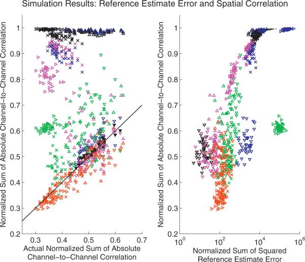
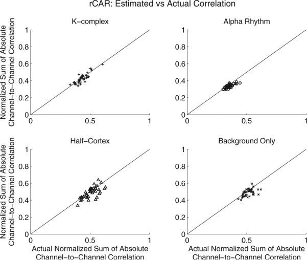
The proposed robust referencing procedure (rCAR, red) out-performs the competing re-referencing procedures by avoiding badly biased estimates of the reference, r_t. Both plots: color indicates re-referencing procedure: C2 (green), CAR (blue), REST-C2 (magenta), REST-CAR (black), and the proposed re-referencing procedure, rCAR (red). Symbol indicates the simulation scenario: K-complex (x), alpha rhythm (right-oriented triangle), active half-cortex (upward-oriented triangle), and random cortical source activity over the whole cortex labeled background only, (downward-oriented triangle). Together these scenarios investigate the performance of the re-referencing procedures on increasingly non-focal cortical activity. Each mark indicates the result of a single simulation for a single re-referencing procedure. Forty simulations are performed for each simulation scenario. For a complete description of the simulations, including a description of the simulation scenarios, see Section 3.1. Left: actual sum of the absolute channel-to-channel correlation (computed from the synthetic silent-reference recordings) vs. the sum of the absolute channel-to-channel correlation estimated from the re-referenced synthetic data produced in simulation. The proposed robust reference procedure (rCAR, red) avoids badly biased correlation estimates computed using the competing references. Right: the sum of the absolute channel-to-channel correlation (vertical axis) tends to increase with increasing reference estimator error. The standard deviation normalized reference estimator error is estimated (horizontal axis) from synthetic data as the scaled sum of the squared deviations of the reference estimate,r̂_t, from the actual reference, r_t, divided by the product of the channel standard deviations, σ_kσ_k′. This quantity directly estimates $\frac{MS{E}_e}{{\sigma }_k{\sigma }_{k^{\prime }}}$ appearing in Eq. (C.11). As expected from Eq. (C.11), the sum of the absolute channel-to-channel correlations tends to increase with the scaled reference estimator error. This result, established in simulation for a known r_t, is used to establish a performance metric for the competing re-referencing procedures when re-referencing real data where r_t is not known. The sum of the absolute channel-to-channel correlations for actual data are plotted in Fig. 9. The proposed re-referencing procedure, rCAR, is always fairly accurate and does not exhibit the large bias demonstrated by the competing re-referencing procedures in at least one simulation scenario. (For interpretation of the references to color in this legend, the reader is referred to the web version of the article.)

2.4. Robust estimation

The topic of robust estimation – a classical area of study in statistics – is documented in many works. These include the books Maronna et al. (2006), Hampel et al. (2011), Huber (1964, 1996), and the review papers Huber (1972), Hampel (2001). While there are many results providing measures of “statistical robustness” – heuristically a robust estimator is one that estimates a model parameter in such a way that when the actual data is drawn from a statistical model different from the one for which the estimator is designed, the performance of the estimator degrades in a controlled fashion. As discussed in Section 2.1, and with respect to the common-average reference estimator, ${\widehat{r}}_t^{\left(CAR\right)}$, which is mean-square error optimal for estimation of the reference, r_t in Eq. (1) when s_t,k is zero for each channel k, CAR is model mis-matched for those time-indices where the s_t,k are non-zero (it is biased when ${\sum }_{k=1}^{N_c}{s}_{t,k}\ne 0$). In this scenario, it is desirable to replace CAR with an estimator robust to the “contaminating signals” s_t,k. The robust CAR (rCAR) estimator is obtained by replacing the CAR estimator of the reference, ${\widehat{r}}_t^{\left(CAR\right)}$, with a robust estimator called a re-descending M-estimator, ${\widehat{r}}_t^{\left(rCAR\right)}$. Briefly, instead of minimizing the sum of squared deviations, as done by the sample average, an M-estimator, that is, a maximum-likelihood type estimator, minimizes the sum of a function of the deviations chosen to have advantageous properties (for example, Maronna et al., 2006). When the function applied to the deviations is appropriately chosen, it introduces a resistance of the resulting estimator to data values that deviate substantially from the estimate with respect to an appropriately chosen scale. Phrased differently, this estimator resistance is obtained by down-weighting the contribution of improbable measurements to the robust estimator.

In the current situation, improbable measurements tend to occur when the ideal voltage recording, s_t,k deviates substantially from zero. Thus, the robust procedure introduces a signal dependent down-weighting of measurements in an estimate of the reference. Because, effectively, the number of channels involved in any estimate of the reference at a given sampling instant changes with time, so does the variance of the resulting reference estimator. Because of this non-stationary effect frequent “jumps” occur on all of the channels due to the re-referencing procedure when a large signal is present. When the signal is smaller, the variance of the reference estimator is lower, and the jumps are less frequent. These events that affect all channels with a signal dependent rate of occur-rence are avoided by applying the M-estimator on a per-frequency basis to the discrete Fourier transformed data. The specification of the proposed robust reference estimator, ${\widehat{r}}_t^{\left(rCAR\right)}$, is detailed in Appendix B. For convenience, Appendix B also includes a summary of the proposed robust procedure.

It is important to note that while ${\widehat{r}}_t^{\left(rCAR\right)}$ is robust to focal neural activity, s_t,k can introduce activity that ${\widehat{r}}_t^{\left(rCAR\right)}$ is not robust to. Specifically, when s_t,k contributes to all of the channels equally it is indistinguishable from reference activity. Similarly, when s_t,k exhibits random behavior with a large standard deviation on the majority of channels, this “noise” is attributed to the sensor variance, ${\sigma }_n^2$. This latter effect, while increasing the variance of the reference estimators, is only serious when this increase is time-dependent and when computing${\check{r}}_t^{\left(rCAR\right)}$ using data where this temporal change occurs. In this case, ${\widehat{r}}_t^{\left(rCAR\right)}$ possesses a time-independent variance which is at times inconsistent with the time-dependent variance of the data. This effect, present in, for example, neural data containing the onset of spike-wave complexes or seizures, is dealt with by computing${\check{r}}_t^{\left(rCAR\right)}$ on a sliding window basis consistent with an assumption of local stationarity. The performance of this latter sliding-window ${\widehat{r}}_t^{\left(rCAR\right)}$ estimator is investigated on the onset of the spike-wave complex (Section 3.3, Fig. 10).

Fig. 10.

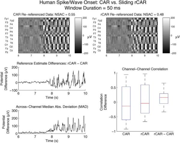
The proposed sliding window version of ${\widehat{r}}_t^{\left(rCAR\right)}$ successfully re-references dramatically non-stationary data. The CAR (upper-left) and rCAR (upper-right) re-referenced onset of the 3 Hz bifrontal spike wave complex. This analysis is identical to that used to re-reference the spike wave complex depicted for seconds 10–12.5 in Figs. 7 and 8, except that ${\widehat{r}}_t^{\left(rCAR\right)}$ is computed using the sliding window (50 ms duration) procedure discussed in Section 2.4, for seconds 6–10 as opposed to ${\widehat{r}}_t^{\left(rCAR\right)}$ computed using all of the data from second 10 to second 12.5. Upper left: CAR re-referenced data. Upper right: rCAR re-referenced data. The normalized sum of absolute correlations (NSAC), plotted for the synthetic data in Fig. 3 and for the real data in Fig. 9, is again larger for CAR than for the sliding version of rCAR and is similar to values found in both the previous simulations and in the previous data analysis. Middle left: the difference between the rCAR and CAR reference estimates. The variance of the differences is consistent with the change in the across-channel variance (bottom left), as measured with the median of the across-channel absolute deviations from the across-channel median (MAD). The change in MAD at around second 8 signifies a dramatic change in the across-channel variation. Note that the MAD measure of variability is not affected by dramatic variability present on less than half of the channels. Lower right: Whisker-box plots of the 171 channel-to-channel pairwise correlations computed from the CAR re-referenced data 1st column), computed from the sliding rCAR re-referenced data (2nd column) and the difference between the pairwise correlations: rCAR - CAR (3rd column). Note that the very large negative correlations present with CAR are absent with sliding rCAR, and the median of the pairwise correlations computed using the CAR re-referenced data is lower than the median of the pairwise correlations computed using sliding rCAR. This manifests in the pairwise correlation difference (rCAR-CAR) exhibiting a positive bias – as expected due to the ability of rCAR to avoid the spatially distributed negative correlation exhibited by data re-referenced with CAR.

3. Results

This paper introduces a robust EEG re-referencing procedure (Section 2.4) that performs well in all tested scenarios and maintains this performance in scenarios where competing procedures fail dramatically. This performance is demonstrated in simulation in Sections 3.1 and 3.2 and with actual data in Sections 3.3 and 3.4. The proposed robust re-referencing procedure avoids signal dependent spatial correlation that arises when applying existing re-referencing procedures to recordings exhibiting strongly activated channels.

This work introduces robust statistical estimation to the EEG re-referencing literature and establishes the relation, Eq. (C.11), linking channel-to-channel correlation with the accuracy of the reference estimator implicit in any given re-referencing procedure. This relation re-states Eq. (6) of Hu et al. (2010) in a fashion suitable for the analysis performed here and facilitates the development of an assay that is used to judge the quality of the re-referencing procedures on human EEG recordings in which the true reference is unknown.

3.1. Simulation

To exhibit features and performance of the proposed robust CAR (rCAR) re-referencing procedure, four EEG scenarios are simulated. Each scenario produces a different, common and stylized EEG phenomenon. For each of these stylized EEG recordings, the physical (C2), the common-average reference (CAR) (Section 2.2), the reference standardization technique with respect to the physical reference (REST C2) (Section 2.3), the reference standardization technique with respect to CAR (REST CAR) (Section 2.3), and the proposed robust CAR (rCAR) (Section 2.4), are employed and the resulting re-referenced data compared against the ideal, silent-reference recordings. Note that in these simulations REST is computed using a perfectly specified forward model. Because of this, the true performance of REST is likely worse.

For each scenario, forty sessions worth of standard 19 channel EEG data are created. To produce each EEG recording, 3521 cortical dipoles are distributed evenly over a spherical hemisphere modeling the cortical surface. The employed tessellation is realized with the aid of the EasySpin set of MATLAB functions (Stoll (2003, ch. 4), & Stoll and Schweiger (2006)). The forward model, G, relating the activity of the cortical dipoles, c_t, to the ideal recordings, s_t according to Eq. (10), is specified using a three spherical shell model as described in Nunez and Srinivasan (2006) with parameters specified in Appendix D.

The pseudo-inverse G⁺ of the forward model G, described in Section 2.3, is used to relate desired, channel-specific responses to actual cortical dipoles. That is, for every scenario, the time-series for each of the active channels is specified, and G⁺ applied to invert the sensor time-series to obtain cortical dipole time-series. These cortical sources are then added to noise with a 1/f spectrum, propagated back to sensor space with G and then incremented with sensor noise. The standard deviation of the sensor noise is specified to be √2 μ V consistent with (Neurophysiology, 2006).

Each of the four scenarios simulate a different type of EEG recording. The scenarios are (1) a single K-complex consisting of a brief, large amplitude 750 ms with unequal voltage on multiple channels, (2) an alpha rhythm consisting of moderate amplitude 10 Hz oscillations on a few channels, (3) recordings resulting from broadly distributed cortical activity (5 Hz tapered oscillations active on one-half of the channels), and (4) recordings that result from noisy, temporally correlated and spatially independent activity over the entire cortex (i.e., “background-only” dipole source activity). Together these scenarios investigate the performance of the re-referencing procedures on increasingly non-focal cortical activity of varying amplitude, duration, and spatial distributions.

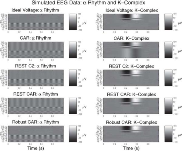
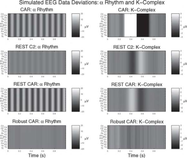
For each of the forty simulations in each of the four scenarios, the physical C2 reference, the common-average reference (CAR, Section 2.2), the REST-C2 and REST-CAR referencing procedures (Section 2.3), and the proposed robust re-referencing procedure (rCAR, Section 2.4) are computed and their performance compared. Examples of the re-referenced data are plotted for the alpha rhythm and K-complex scenarios in Fig. 1, and the deviation of the re-referenced data from ideal is plotted in Fig. 2.

Fig. 1.

Example synthetic re-referenced data illustrate the utility of rCAR. Simulation results are summarized in Section 3.2 and described in detail in Section 3.1. Left: simulated α rhythms in posterior electrodes. Right: simulated K-complex (a brief, oscillatory event). Top row: ideal voltage, s_t defined in Section 2.1. Remaining rows: competing re-referencing procedures. The proposed re-reference procedure (rCAR) (Section 2.4) out-performs all of the re-reference procedures in the posterior alpha rhythm and K-complex cases (see also Fig. 3). The proposed re-reference procedure (rCAR) does not “bleed” channel signal across channels. This feature of the rCAR procedure restricts large signals on some channels from affecting other channels and is, heuristically speaking, the essence of its success. It is demonstrated more clearly in Fig. 2, where the ideal EEG recordings are removed from the re-referenced data and the resulting difference is displayed.

Fig. 2.

Example synthetic re-referenced data resulting from the simulations described in Section 3.1 reduced by the ideal channel recordings to highlight their differences. The simulations are identical to those used to produce Fig. 1. Ideally, these images would be zero for all times and channels. A departure from zero indicates an error in the re-referencing procedure. The across-channel “bleeding” effect described in the text and in Fig. 1 is apparent. The proposed re-referencing procedure (rCAR) is the most accurate. The vertical stripes result from the fact that the reference effects all of the channels equally in the data model, Eq. (1). When the estimate of the reference deviates from the actual reference the result is an equal error on all of the channels.

Associated with the re-referenced data are the corresponding estimates of the physical C2 reference time-series. For each estimate of the reference time-series (one estimate for each of the forty simulations for each of the four simulation scenarios) the average-squared deviation of the estimated reference time-series from the actual, physical C2 reference time-series is computed, along with the sum of the absolute pairwise channel-to-channel correlation estimated from the re-referenced recordings. To assess the accuracy of the competing re-referencing procedures when estimating channel-to-channel correlation, the actual sum of absolute pairwise channel-to-channel correlation is computed from the ideal, silent-reference recordings. These three quantities are plotted against each other in Fig. 3. Each dot in Fig. 3 results from the use of a single re-referencing procedure with the time-series realized in one of the forty EEG recording realizations for one of the four EEG scenarios. Because of the random cortical background to which the more focal activity is added, as well as the random sensor noise, the estimates fluctuate from one simulation to another. This set of simulations confirms the relation between the sum of the absolute channel-to-channel correlation and the error of the reference estimator, Eq. (C.11), associated with any given re-referencing procedure (Fig. 3, right). Further, the accuracy of pairwise channel-to-channel correlation computed from the various re-referenced data is explored (Fig. 3, left and Fig. 4). When computed from the robust re-referenced data the pairwise correlation accurately approximates the actual pairwise correlation in all scenarios considered here (Fig. 4). Each of the other competing re-referenced procedures fail dramatically in at least a single simulation scenario (Fig. 3).

Fig. 4.

The simulation results for the proposed robust re-reference procedure (rCAR) presented in Fig. 3, reproduced for clarity. The proposed robust referencing procedure yields unbiased estimates of the channel-to-channel correlation in the four simulation scenarios.

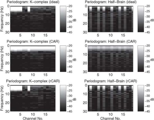
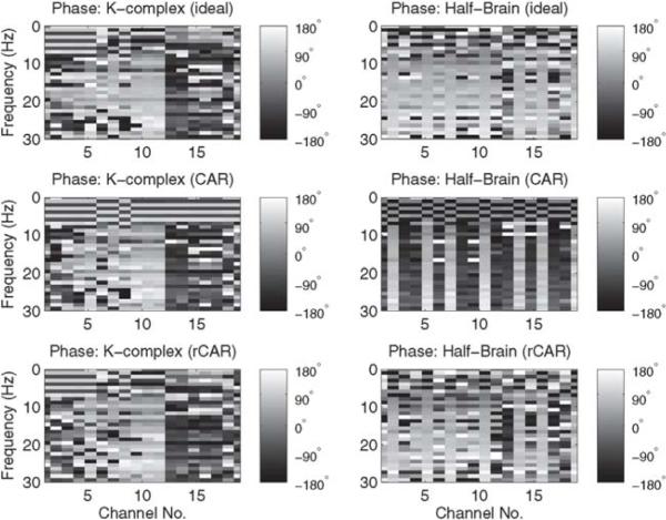
Finally, to directly investigate the effects of the rCAR and CAR re-referencing procedures in the frequency domain, the magnitude and phase of the discrete Fourier transformed re-referenced data are plotted. In Fig. 5 the periodogram of the re-referenced recordings is compared against the periodogram of the ideal, silent-reference recordings. The rCAR re-referencing procedure more faithfully reproduces the periodogram of the silent-reference recordings. In Fig. 6 the phase of the discrete Fourier transformed re-referenced recordings are compared against the phase of the discrete Fourier transformed ideal, silent-reference recordings. The rCAR re-referencing procedure more faithfully reproduces the phase of the silent-reference recordings.

Fig. 5.

The periodogram of the CAR and rCAR re-referenced data. The periodogram of rCAR is more similar to the periodogram of the ideal silent-reference recordings than the periodogram of the CAR. In particular, the low-frequency streaking across the channels present in the CAR re-referenced data is absent in the rCAR re-referenced data.

Fig. 6.

The phase of the discrete Fourier transformed CAR and rCAR re-referenced data. The phase of rCAR is more similar to the phase of the ideal silent-reference recordings than the phase of the CAR recordings.

3.2. Summary of simulation study results

The following is a summary of the main results drawn from the simulated scenarios in Section 3.1. These scenarios demonstrate features that occur in EEG recordings and are made prominent through a complicated simulation procedure involving the inversion of a concentric 3-layer spherical shell model linking cortical activity with measurements (using methods adapted from Nunez and Srinivasan (2006) and described in Section 3.1). The purpose of these simulations is to demonstrate the good performance of the proposed re-referencing procedure, even in these scenarios. The simulation results are shown in Figs. 1–3 and are detailed below:

• All of the re-referencing procedures fail dramatically for at least one EEG recording scenario except the proposed rCAR re-referencing procedure (Figs. 1–3).

• The proposed rCAR re-referencing procedure yields the most accurate channel-to-channel correlation (Fig. 3, left), for the simulated K-complex and alpha rhythm scenarios.

• The proposed rCAR re-referencing procedure is associated with the most accurate reference estimates (Fig. 3, right), for the simulated K-complex and alpha rhythm scenarios. This is also visible by eye in examples of the simulated re-referenced data (Figs. 1–2).

• The sum of the absolute channel-to-channel correlation is correlated with reference estimator accuracy, as shown in Fig. 3 and in Eq. (C.11). While correlated, the more accurate relation is sigmoidal (Fig. 3, right) and complicated (Eq. (C.11)).

3.3. Empirical human data

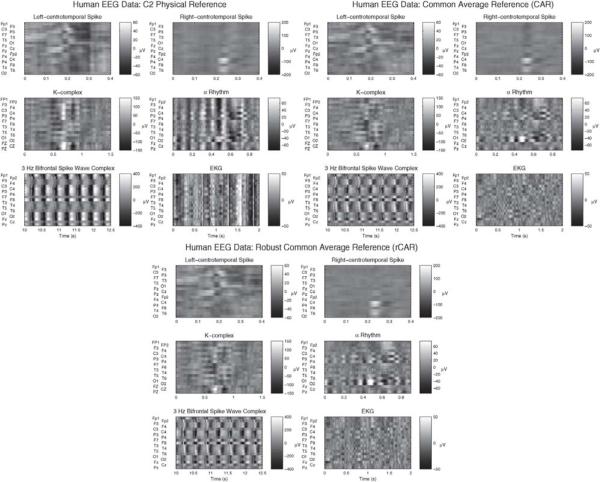
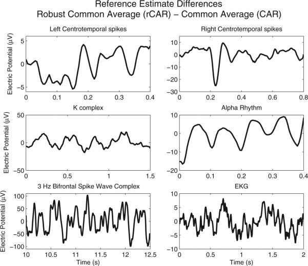
To further determine the efficacy of the competing re-referencing procedures, clinical 19-channel EEG recordings are analyzed. Six intervals of EEG data filtered to the 1–50 Hz interval of frequencies were selected to capture common features of human EEG recordings, with a range of spatial distributions, durations, and amplitudes. For each of the selected scenarios, the true distribution of the voltage activity is known or has been modeled. These include (1) left and (2) right centrotemporal spikes with a horizontal dipole (Pataraia et al., 2008), (3) the K-complex (Wennberg, 2010), (4) posterior dominant alpha rhythms (Michel et al., 1992), (5) 3 Hz bifrontal spike wave complex and (6) electrocardiogram (EKG) contamination. The re-referenced 19-channel EEG data is depicted in Fig. 7. The difference between the rCAR estimated reference time-series and the CAR estimated reference time-series is depicted in Fig. 8. Substantial differences exist between the various re-referenced EEG recordings and could introduce differences into subsequent EEG analyses.

Fig. 7.

The 19-channel EEG data recorded with respect to the C2 physical reference (upper-left), CAR (upper-right), and rCAR (bottom). For each panel, clockwise from upper left: a left centrotemporal spike (t = 0.2 s), a right centrotemporal spike (t = 0.21 s), a posterior dominant alpha rhythm, an example of EKG activity, a run of generalized spike and wave activity, and a K-complex (t = .65 s). The data has been bandpass filtered prior to re-referencing to the 1–50 Hz band of frequencies. Vertical streaking prominent when using the CAR re-referenced data for the right centrotemporal spike, the K-complex and the alpha rhythm (t = .41 s), is reduced or absent when re-referencing with rCAR, while the good behavior of CAR is maintained when re-referencing the EKG artifact.

Fig. 8.

The difference in the proposed (rCAR) estimate of the unknown reference time-series r_t and the estimate of the r_t time-series associated with CAR. Substantial differences exist between${\check{r}}_t^{\left(rCAR\right)}$ and${\check{r}}_t^{\left(CAR\right)}$ for the six different 19-channel EEG data examples.

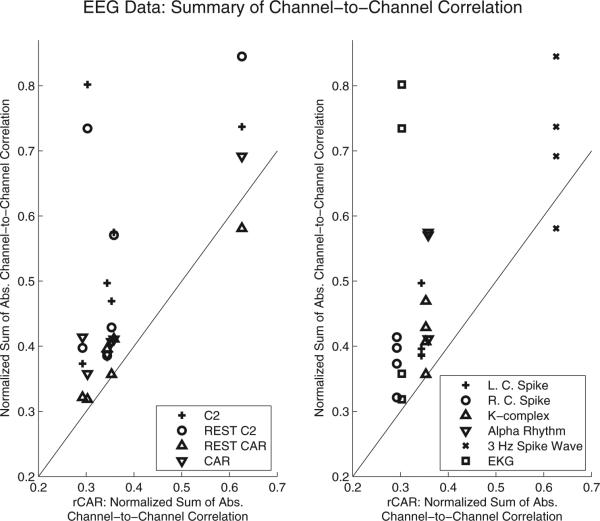
By comparing the sum of the absolute channel-to-channel correlation computed with the re-referenced data to the sum of the absolute channel-to-channel correlation computed with the proposed re-referenced data (rCAR), a sense for the relative accuracy of the competing re-referencing procedures is established. Key to this establishment is the theoretical relation, Eq. (C.11), linking the sum of the absolute channel-to-channel correlation with the scaled mean-square error of each reference estimator, and the supporting simulation results corroborating the theoretical result (Section 3.1). The competing re-referencing procedures yield sum of absolute channel-to-channel correlation that exceed that obtained with the proposed re-referencing procedure (rCAR), suggesting superior rCAR reference estimator accuracy (Fig. 9).

Fig. 9.

The sum of the absolute channel-to-channel correlations with the proposed re-referenced data (rCAR) is lower than the absolute channel-to-channel correlations estimated in nearly all scenarios. The two panels illustrate the same results with symbols indicating different references (left) and symbols indicating different EEG activity patterns (right).

As discussed in Section 2.4, when more than half of the channels exhibit neural activity with a time-dependent variance, ${\widehat{r}}_t^{\left(rCAR\right)}$ computed from all of the data can exhibit a constant variability inconsistent with the time-dependent across-channel variability of the data. This effect is reduced by employing a sliding ${\widehat{r}}_t^{\left(rCAR\right)}$ where the reference estimates are computed for short, overlapping durations. The effectiveness of this procedure is compared against the CAR re-referencing procedure for the onset of the spike wave complex depicted for the CAR and rCAR referenced data in the upper row of Fig. 10. The sliding robust reference procedure, computed using a sliding window (50 ms duration), out-performs CAR in a fashion consistent with the previous results depicted in Figs. 7 and 8. In particular, the sliding robust re-referencing procedure avoids the negative correlation introduced by use of the common-average reference (Fig. 10, lower-right).

3.4. Summary of EEG analysis results

By analyzing re-referenced clinical EEG data, the following conclusions are drawn. With few exceptions, the proposed rCAR re-referencing procedure yields the lowest sum of the absolute channel-to-channel correlations (Fig. 9). This result, along with Eq. (C.11) and the simulation results presented in Section 3.2 linking the reference estimator accuracy with a reduced sum of absolute channel-to-channel correlation, suggest that rCAR re-referencing usefully approximates the actual ideal re-referenced data in all scenarios.

In any given EEG analysis, the observed brain dynamics are not known prior to analysis. Expert review of EEG data may allow an appropriate choice of reference. However, brain voltage activity is dynamic so different features may appear within a single recording, necessitating a dynamic reference choice. In addition, voltage tracings with diverse or subtle focal features may exhibit unforeseen inaccuracies using current re-referencing techniques. Consequently, it may be unwise to use an EEG re-referencing procedure that can fail dramatically in some scenarios. Each of the existing EEG re-reference procedures analyzed in this paper fail dramatically in at least one simulation scenario (Fig. 3). The proposed re-referencing procedure (rCAR) is a safe and efficient alternative.

4. Discussion

In this work, the re-referencing procedures are evaluated based upon their ability to approximate “silent reference recordings”. This ability is determined by the bias of the estimators associated with each of the re-referencing procedures, and this bias is controlled by the influence of small numbers of channels. By down-weighting the influence of any few electrodes upon the reference estimate in a specific fashion determined by the principles of robust statistical estimation, the proposed robust procedure is developed. Because of this “principle of robust estimation” it suffices to establish the bias properties of the reference estimators. This is done in simulation, and further, the effectiveness is demonstrated with actual data.

The novel robust re-referencing procedure performs well for a wide range of EEG recording scenarios, and avoids dramatic inaccuracies exhibited by competing re-referencing procedures. Specifically estimating channel-to-channel dependency, the correlation bias exhibited by existing re-reference estimators makes their use problematic. This difficulty extends to derivative quantities such as networks and their associated statistics.

While superior performance of the proposed re-referencing procedure is established in this work, some limitations exist. One of the main limitations of the common average reference is the impact of large focal voltage fluctuations on the reference estimate, leading to erroneously active measures of relatively quiescent brain regions. By effectively down-weighting the contributions to the reference estimate from local cortical activity, the proposed robust reference mitigates these errors. This decoupling reduces activity dependent reference estimate bias but at the price of increased, and activity-dependent, reference estimator variance. This trade is usually desirable, as the bias of comparable procedures can be substantial (Figs. 1 and 2). Moreover, more trials and averaging can reduce an increased variance to desired levels, whereas the correction of a signal-dependent bias cannot be done.

Beyond this trade-off between bias and variance, two limitations of the proposed re-referencing procedure exist. First, a performance bound exists common to all of the references considered in this paper. When neural signal affects all of the channels equally, it is not possible, without further information, to separate the relative contributions of neural signal and reference. Second, as discussed in Section 2.4, when the variability of broadly distributed neural activity changes dramatically in time, the resulting robust reference estimator can exhibit inappropriate variability. While this effect is effectively mitigated by performing the robust re-referencing procedure in a temporally adaptive fashion, the price paid for temporally resolving the spatially broad changing signal variance is a re-introduction of the possibility of a signal-dependent variance. In this work we have focused on removing contaminating reference effects from the scalp EEG signal in the common clinical scenario in which only sparse electrode sampling is available. In doing so, we have emphasized the effectiveness of the methodology in the 19 channel case in theory, simulation and practice. It is via the bias in the reference estimators that the reference-effect occurs and reducing this bias reduces the reference effect. This work is of high practical value for improving the accuracy of the low density scalp EEG recording which is commonly employed in patient care.

HIGHLIGHTS.

• A novel procedure is introduced based upon robust statistical estimation to mitigate EEG reference effect.

• The new procedure can reduce bias, as is demonstrated in simulation and with human EEG recordings.

• Subsequent inter-regional coupling estimates can be improved.

• The procedure is simple and fast.

Summary: robust re-referencing procedure.

1. Choose an analysis window duration to use with the short-time Fourier transform.

2. Compute the short-time Fourier transform (STFT) associated with each EEG channel.

3. For every time and frequency, compute the median of the absolute deviations (MAD) of the real and imaginary parts of the STFT.

4. For every time and frequency, solve Eqs. (B.8) and (B.9) using the MAD computed in Step 3 and the STFT computed in Step 2.

5. Add the solution to Eqs. (B.8) and (B.9) to the STFT.

6. For each time at which the STFT is computed, inverse discrete Fourier transform the augmented STFT computed in Step 5.

7. The inverse DFTs (across-channels) evaluated at the epoch-center is the robust re-referenced data for this time-step.

8. Done.

Appendix A. REST reference estimator ${\widehat{s}}_t^{\left(REST\right)}$

Let ${\tilde{\mathbf{d}}}_t^{\left(\tilde{r}\right)}$ be the vector of scalp potential-differences recorded with respect to an unspecified physical reference r̃_t at time-index t when there is no sensor noise (n_t,k = 0). Here ~ is used to indicate noiseless data, and the kth element of ${\tilde{\mathbf{m}}}_t^{\left(\tilde{r}\right)}$ equals the observed measurement, m_t,k, associated with d_t,k, the kth element of ${\mathbf{d}}_t^{\left(r\right)}$, when the sensor noise is zero. In ${\mathbf{d}}_t^{\left(r\right)}$ the use of the actual reference is denoted by the ^(r).

$${\left({\tilde{\mathbf{d}}}_t^{\left(\tilde{r}\right)}\right)}_k=s_{t,k}-{\tilde{r}}_t.$$ (A.1)

When only the dipole sources c_t contribute to the reference electric field the reference can be described by the cortical activity and Eq. (A.1) can be re-written in vector form:

$$\begin{array}{cc}\hfill {\mathbf{m}}_t^{\left(\tilde{r}\right)}=& {\mathbf{s}}_t-{\tilde{r}}_{t}1,\hfill \\ \hfill =& {\mathbf{Gc}}_t-G_{\tilde{r}}{\mathbf{c}}_t,\hfill \\ \hfill =& (\mathbf{G}-{\mathbf{G}}_{\tilde{r}}){\mathbf{c}}_t.\hfill \end{array}$$ (A.2)

Here 1 is a vector of N_c ones, and G_r̃ is a N_c by N_s dimensioned vector that maps the cortical dipoles to the reference channel, r̃_t1. The matrix difference G − Gr̃ is, in general, not invertible. However, one can choose a candidate inverse, A, from the infinitely many possible inverses so that

$${\widehat{\mathbf{c}}}_t=\mathbf{A}{\tilde{\mathbf{d}}}_t^{\left(\tilde{r}\right)},$$ (A.3)

and

$$\begin{array}{cc}\hfill {\tilde{\mathbf{d}}}_t^{\left(\tilde{r}\right)}=& (\mathbf{G}-{\mathbf{G}}_{\tilde{r}}){\widehat{\mathbf{c}}}_t,\hfill \\ \hfill =& (\mathbf{G}-{\mathbf{G}}_{\tilde{r}})\mathbf{A}{\tilde{\mathbf{d}}}_t^{\left(\tilde{r}\right)},\hfill \end{array}$$ (A.4)

such that the 2-norm of ĉ_t is minimum. This is called the minimumnorm solution to the under-determined problem³ Eq. (A.2), and is obtained by picking A to be the pseudoinverse of G – G_r̃:

$$\mathbf{A}={(\mathbf{G}-{\mathbf{G}}_{\tilde{r}})}^{+}$$ (A.5)

where the pseudoinverse is denoted by superscript ‘+’. See Scharf (1991, p. 394) and Hämälä inen and Ilmoniemi (1994) for a discussion of the minimum-norm solution in this context.

By adding noise to d̃^(r̃), REST can be phrased in terms of estimators and estimates as discussed in Section 2.1. Let ${\mathbf{d}}_t^{\left(\tilde{r}\right)}{\tilde{\mathbf{d}}}_t^{\left(\tilde{r}\right)}+{\mathbf{n}}_t$, where kth element, (n_t)_k, of n_t is n_t,k defined after Eq. (1). Then ${\left({\mathbf{d}}_t^{\left(\tilde{r}\right)}\right)}_k=d_{t,k}$ when r̃_t = r_t. Then the minimum-norm estimator of the dipole sources,ĉ_t, is,

$${\widehat{\mathbf{c}}}_t={[\mathbf{G}-{\mathbf{G}}_{\tilde{r}}]}^{+}{\mathbf{d}}_t^{\left(r\right)},$$ (A.6)

and an estimator,${\widehat{\mathbf{s}}}_t^{\left(REST\right)}$, of the ideal recordings, s_t is obtained,

$$\begin{array}{cc}\hfill {\widehat{\mathbf{s}}}_t^{\left(REST\right)}=& \mathbf{G}{\widehat{\mathbf{c}}}_t,\hfill \\ \hfill =& \mathbf{G}{[\mathbf{G}-{\mathbf{G}}_{\tilde{r}}]}^{+}{\mathbf{d}}_t^{\left(r\right)}.\hfill \end{array}$$ (A.7)

By combining Eq. (1) with Eq. (A.7), the REST estimator,${\widehat{\mathbf{s}}}_t^{\left(REST\right)}$, of the ideal EEG measurements, s_t, is,

$$\begin{array}{cc}\hfill {\widehat{\mathbf{s}}}_t^{\left(REST\right)}=& \mathbf{G}{[\mathbf{G}-{\mathbf{G}}_{\tilde{r}}]}^{+}({\mathbf{s}}_t-r_{t}1+{\mathbf{n}}_t),\hfill \\ \hfill =& \mathbf{G}{[\mathbf{G}-{\mathbf{G}}_{\tilde{r}}]}^{+}({\mathbf{s}}_t-{\mathbf{n}}_t)-r_t\mathbf{G}{[\mathbf{G}-{\mathbf{G}}_{\tilde{r}}]}^{+}1.\hfill \end{array}$$ (A.8)

Note that r̃_t does not need to coincide with r_t. When the following conditions are met${\check{\mathbf{s}}}_t^{\left(REST\right)}$ is an accurate estimate of the ideal recordings, s_t:

• n_t,k is zero for all of the channels.

• [G − G_r]⁺ accurately approximates G⁻¹.

• 1 lies in the right null-space of G[G Gr̃]⁺ such that the second term in Eq. (A.8) is zero. −

• The reference channel responds only to cortical sources.

The REST re-referencing procedure is applied in simulation in Section 3.2 and to actual EEG recordings in Section 3.4, using a three concentric spherical-shell model of the brain to approximate the forward, G and G_r matrices. This model is further described in Appendix D.

Appendix B. Robust reference estimator ${\widehat{s}}_t^{\left(rCAR\right)}$

In the following a derivation of ${\widehat{s}}_t^{\left(rCAR\right)}$ the proposed robust reference estimator is provided. It is computed as the inverse discrete Fourier transform of its frequency domain counterpart, ${\widehat{R}}_f^{\left(rCAR\right)}$ A summary of the computation is provided in Procedure 1.

At each frequency, f, an estimate of the discrete Fourier transformed reference,${\check{R}}_t^{\left(rCAR\right)}$ is obtained. Here f, in units of cycles/sample, is an integer multiple of $\frac{1}{N_s}$ where N_s is the length of the data under consideration. This estimate is then inverse discrete Fourier transformed to obtain the reference estimate${\check{r}}_t^{\left(rCAR\right)}$. When performing the robust reference estimation in the frequency domain, the signal dependent variance is equivalent to “coloring” the spectrum of the white noise, n_t,k. This coloring does not affect smoothness properties of the re-referenced data and is preferable to the time-domain alternative.

Consider the discrete Fourier transform, D_f,k, of the data, d_t,k, defined in Eq. (1):

$$D_{f,k}=S_{f,k}-R_f+N_{f,k}.$$ (B.1)

The capital letters denote discrete Fourier transformed quantities of the signal (S(f, k), reference (R(f, k)) and noise (N(f, k)). Specifically,

$$D_{f,k}=\sum _{t=0}^{N-1}{d}_{t,k}{e}^{-i2\pi ft},$$ (B.2)

$$S_{f,k}=\sum _{t=0}^{N-1}{s}_{t,k}{e}^{-i2\pi ft},$$ (B.3)

$$R_f=\sum _{t=0}^{N-1}{r}_t{e}^{-i2\pi ft},$$ (B.4)

$$N_{f,k}=\sum _{t=0}^{N-1}{n}_{t,k}{e}^{-i2\pi ft}.$$ (B.5)

Note that the discrete Fourier transformed quantities, for example D_f,k, are equal to a sum of their real and imaginary parts:

$$D_{f,k}=\mathrm{Re}\left\{D_{f,k}\right\}+i\mathrm{Im}\left\{D_{f,k}\right\}.$$ (B.6)

Re {x} and Im {x} are respectively, the real and imaginary part of the complex variable, x.

When s_t,k is equal to zero, so is S_f,k. Then D_f,k possesses a circularly symmetric normal probability density function⁴(Kay, 1993):

$$D_{f,k}\sim \mathcal{C}\mathcal{N}(R_f,{\sigma }_{f,k}^2).$$ (B.7)

The variance, ${\sigma }_{f,k}^2$, is equal to $N{P}_{f,k}^{\left(n\right)}$ where $P_{f,k}^{\left(n\right)}$ is the unknown spectrum of the weak-sense stationary noise, n_t,k. Because the noise spectrum is unknown, σ_f,k is taken to be constant across channels and is robustly estimated from the data as a function of the frequency, f. Specifically, ${\sigma }_{f,k}^2$ is specified to be independent of k and is equal to ${\sigma }_f^2$. Circularly symmetric normal random variables possess independent real and imaginary components, each with one-half the variance of the circularly-symmetric random variable.

The estimator, ${\widehat{R}}_f^{\left(rCAR\right)}$ is constructed by applying the robust M-estimator to both the real and imaginary parts of d̂_f,k separately, such that the following equations are satisfied:

$$\sum _{j=1}^{N_c}\rho \left(\frac{\mathrm{Re}\left\{D_{f,j}\right\}+\mathrm{Re}\left\{{\widehat{R}}_f^{\left(rCAR\right)}\right\}}{{\widehat{\sigma }}_f∕2}\right)=0,$$ (B.8)

$$\sum _{j=1}^{N_c}\rho \left(\frac{\mathrm{Im}\left\{D_{f,j}\right\}+\mathrm{Im}\left\{{\widehat{R}}_f^{\left(rCAR\right)}\right\}}{{\widehat{\sigma }}_f∕2}\right)=0.$$ (B.9)

Here, ρ is Tukey's bisquare function (also known as Tukey's biweight function) (Press et al., 1992). Specifically,

$$\rho \left(x\right)=\{\begin{array}{cc}x{\left(1-{\left(\frac{x}{c}\right)}^2\right)}^2,\hfill & \mid x\mid \le c\hfill \\ 0,\hfill & \mid x\mid >c\hfill \end{array}\phantom{\}}.$$ (B.10)

and ${\widehat{\sigma }}_f$ is a robust estimator of the data scale, σ_f. It is taken to be the median of the absolute deviations of the data from the data median, computed as a function of the frequency f. The parameter c, controlling the down-weighting of deviant data values, is specified to be 2 obtain results presented in this paper. If for example $\mathrm{Re}\left\{D_{f,j}\right\}+\mathrm{Re}\left\{{\widehat{R}}_f^{\left(rCAR\right)}\right\}$ is greater than $c{\widehat{\sigma }}_f∕\sqrt{2}$, then Re {D_f,j} has no influence Re upon $\mathrm{Re}\{{\widehat{R}}_f^{\left(rCAR\right)}$. Fig. B.11 depicts Tukey's bisquare function, ρ(x).

Fig. B.11.

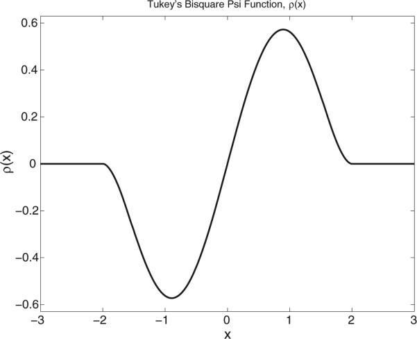
Tukey's bisquare function plotted for c = 2. The re-descending tails down-weight data values that deviate from the theoretical location parameter,–R_f.

Note that if, S_f,k were zero in the model specified by Eq. (B.1), all of the channels could be usefully used to estimate R_f. When s_t,k is equal to zero, the sample average is the maximum likelihood estimator of R_f. The channel down-weighting in the computation of ${\widehat{R}}_f^{\left(rCAR\right)}$ causes the robust estimator variance, $var\left\{{\widehat{R}}_f^{\left(rCAR\right)}\right\}$, to exceed the variance of the sample average estimator. However, in the situation where

$$S_{t,k}=\{\begin{array}{cc}{S}_{f,1}=\Gamma ,\hfill & k=1\hfill \\ S_{f,k}=0,\hfill & k\ne 1\hfill \end{array}\phantom{\}},$$ (B.11)

for |Γ| >> c σ, the bias of the robust estimator, R̂_f , is unaffected by S_f, while the bias of ${\widehat{R}}_f^{\left(CAR\right)}$ is $\frac{\Gamma }{N_c}$. When Γ is small and non-zero, both ${\widehat{R}}_f^{\left(CAR\right)}$ and ${\widehat{R}}_f^{\left(rCAR\right)}$ are biased. As Γ increases the bias of ${\widehat{R}}_f^{\left(CAR\right)}$ increases while the down-weighting performed by ρ(x) begins to have an increasingly large effect – limiting the bias of ${\widehat{R}}_f^{\left(rCAR\right)}$

When Eq. (B.9) is solved frequency by frequency the resulting reference estimator, ${\widehat{R}}_f^{\left(rCAR\right)}$ due to the signal dependent down-weighting of EEG channels contributing to Eq. (B.9), possesses a variance that depends on the frequency index, f. This behavior of ${\widehat{R}}_f^{\left(rCAR\right)}$ introduces a frequency-dependent variability into all of the channels of${\widehat{S}}_{f,k}^{\left(rCAR\right)}$. This effect colors the noise, n_t,k, in a signal dependent fashion, that increases the spectrum of${\widehat{s}}_{t,k}^{\left(rCAR\right)}$ relative to the spectrum of${\widehat{s}}_{t,k}^{\left(CAR\right)}$, but preserves any weak-sense stationary property that the ideal voltage recording might have – only the spectrum is modified, not a time-dependent variance. Besides this theoretical advantage, the robust estimator computed in the frequency domain yields more appealing estimates of s_t,k than a time-domain version. In particular, as previously discussed, a faint, signal-dependent vertical streaking is absent. The performance of ${\widehat{R}}_f^{\left(rCAR\right)}$ versus R̂(CAR) (obtained by transforming ${\widehat{r}}_t^{\left(CAR\right)}$) is explored in simulation in Section 3.1, Figs. 5 and 6. The ${\widehat{R}}_f^{\left(rCAR\right)}$ more faithfully reproduces frequency domain features exhibited by the silent-reference recordings.

From a numerical perspective, solving Eq. (B.9) is challenging. Heuristically this is clear by noting that an unreasonable estimate of R_f, one that is very large relative to the estimated standard deviation, ${\check{\sigma }}_f$ for example, satisfies Eq. (B.9) due to the zeroing of Eq. (B.1) and Eq. (B.10) by the action of ρ(x) for large |x|. In practice Eq. (B.10) is solved numerically through an iterative Newton-Raphson algorithm augmented to include the higher derivatives of Eq. (B.10). This augmented Newton-Raphson algorithm performs exceedingly well on all data used in this paper; typically converging in two iterations to sum-square errors of less than 10⁻²⁰. It is described in Appendix E.

Appendix C. corr ŝ_t,k, ŝ_t,k′

By modeling the unknown ideal EEG recordings, s_t,k, as mean-zero, weak-sense stationary random processes, the sample cross-channel correlation can be related to the theoretical cross-channel correlation. Specifically, let the ideal, reference-free, cross-covariance, C_k,k′ , between channel k and channel k′ be,

$$C_{k,k^{\prime }}=E\left\{s_{t,k}{s}_{t,k^{\prime }}\right\}.$$ (C.1)

Then, the sample estimator,Ĉ_k,k′ of C_k,k′ is,

$$\begin{array}{cc}\hfill {\widehat{C}}_{k,k^{\prime }}=& \frac{1}{n}\sum _{t=0}^{N-1}{\widehat{s}}_{t,k}{\widehat{s}}_{t,k^{\prime }}\hfill \\ \hfill =& \frac{1}{n}\sum _{t=0}^{N-1}\left(d_{t,k}+{\widehat{r}}_t^{\left(type\right)}\right)\left(d_{t,k^{\prime }}+{\widehat{r}}_t^{\left(type\right)}\right),\hfill \\ \hfill =& \frac{1}{n}\sum _{t=0}^{N-1}\left(s_{t,k}+{\widehat{e}}_t+n_{t,k}\right)\left(s_{t,k^{\prime }}+{\widehat{e}}_t+n_{t,k^{\prime }})\right),\hfill \\ \hfill =& \frac{1}{n}\sum _{t=0}^{N-1}{s}_{t,k}{s}_{t,k^{\prime }}+\frac{1}{n}\sum _{t=0}^{N-1}{s}_{t,k}\left({\widehat{e}}_t+n_{t,k^{\prime }}\right)+\frac{1}{n}\sum _{t=0}^{N-1}{s}_{t,k^{\prime }}\left({\widehat{e}}_t+n_{t,k}\right)+\frac{1}{n}\sum _{t=0}^{N-1}\left({\widehat{e}}_t+n_{t,k}\right)\left({\widehat{e}}_t+n_{t,k^{\prime }}\right).\hfill \end{array}$$ (C.2)

The expected channel-to-channel covariance is then,

$$E\left\{{\widehat{C}}_{k,k^{\prime }}\right\}=C_{k,k^{\prime }}^{\left(s\right)}+C_k^{\left(se\right)}+C_{k^{\prime }}^{\left(se\right)}+T_3.$$ (C.3)

Here the ideal, silent-reference channel-to-channel covariance, C^(s)_k,k is,

$$C_{k,k^{\prime }}^{\left(s\right)}=E\left\{s_{t,k}{s}_{t,k^{\prime }}\right\}$$ (C.4)

and the covariance, $C_k^{\left(se\right)}$, between the kth silent-reference recording and the reference estimator error,ê_t, is given by

$$\begin{array}{cc}\hfill C_k^{\left(se\right)}=& E\left\{s_{t,k}\left({\widehat{e}}_t+n_{t,k}\right)\right\},\hfill \\ \hfill =& E\left\{s_{t,k}{\widehat{e}}_t\right\},\hfill \end{array}$$ (C.5)

since E {s_t,kn_t,k} = 0. The last term in Eq. (C.3) can be shown to be:

$$T_3=MS{E}_e+{\delta }_{k,k^{\prime }}{\sigma }_n^2+C_k^{\left(nr\right)}+C_{k^{\prime }}^{\left(nr\right)},$$ (C6)

where MSE_e is the mean-square error of the reference estimator ${\widehat{r}}_t^{\left(type\right)}$,

$$MS{E}_e=E\left\{{\widehat{e}}_t^2\right\}.$$ (C.7)

The mean-square error summarizes the accuracy of an estimator. It is equal to the estimator variance plus the squared bias of an estimator and provides an excellent indication of the typical accuracy of any given estimate. Lower mean-square error estimators indicate that their associated estimates will tend to be more accurate. The reference-estimator dependent term, $C_k^{\left(nr\right)}$, can be specified explicitly for the common-average reference:

$$\begin{array}{cc}\hfill C_k^{\left(nr\right)}=& E\left\{n_{t,k}{\widehat{r}}_t^{\left(CAR\right)}\right\},\hfill \\ \hfill =& E\left\{-\frac{n_{t,k}}{N_c}\sum _{k^{\prime }=0}^{N_c}{d}_{t,k^{\prime }}\right\},\hfill \\ \hfill =& -\frac{1}{N_c}\sum _{k^{\prime }=0}^{N_c}E\left\{n_{t,k}\left(s_{t,k^{\prime }}-r_t+n_{t,k^{\prime }}\right)\right\},\hfill \\ \hfill =& -\frac{{\sigma }_n^2}{N_c}.\hfill \end{array}$$ (C.8)

Although sometimes more complicated, the inverse N_c dependence of this term holds when using the proposed robust reference estimator, ${\widehat{r}}_t^{\left(rCAR\right)}$. The channel-to-channel correlation, ρ_k,k′ , can now be expressed as in Eq. (C.11). The approximation in Eq. (C.11) stems from the fact that,

$${\rho }_{k,k^{\prime }}\approx \frac{C_{k,k^{\prime }}^{\left(s\right)}+C_k^{\left(se\right)}+C_{k^{\prime }}^{\left(se\right)}+MS{E}_e+{\delta }_{k,k^{\prime }}{\delta }_n^2+C_k^{\left(nr\right)}+C_{k^{\prime }}^{\left(nr\right)}}{\sqrt{C_{k,k}^{\left(s\right)}+2C_k^{\left(se\right)}+MS{E}_e+{\sigma }_n^2+C_k^{\left(nr\right)}}\sqrt{C_{k^{\prime },k^{\prime }}^{\left(s\right)}+2C_{k^{\prime }}^{\left(se\right)}+MS{E}_e+{\sigma }_n^2+C_{k^{\prime }}^{\left(nr\right)}}},$$ (C.9)

$$={\rho }_{k,k^{\prime }}+\frac{C_k^{\left(se\right)}+C_{k^{\prime }}^{\left(se\right)}+MS{E}_e+{\delta }_{k,k^{\prime }}{\sigma }_n^2+C_k^{\left(nr\right)}+C_{k^{\prime }}^{\left(nr\right)}}{\sqrt{C_{k,k}^{\left(s\right)}{C}_{k^{\prime },k^{\prime }}^{\left(s\right)}}}+HOTs,$$ (C.10)

$$\approx {\rho }_{k,k^{\prime }}+\frac{C_k^{\left(se\right)}+C_{k^{\prime }}^{\left(se\right)}+MS{E}_e+{\delta }_{k,k^{\prime }}{\sigma }_n^2+C_k^{\left(nr\right)}+C_{k^{\prime }}^{\left(nr\right)}}{{\sigma }_k^{\left(s\right)}{\sigma }_{k^{\prime }}^{\left(s\right)}},$$ (C.11)

The typical channel-to-channel correlation depends upon the mean-square reference estimator error, MSE_e. The term HOTs contains the higher-order terms in the Taylor expansion applied to the first term in Eq. (C.9) to obtain Eq. (C.10). The accuracy of Eq. (C.11) increases with increasing ${\sigma }_k^{\left(s\right)}{\sigma }_{k^{\prime }}^{\left(s\right)}$ and decreases with increasing $C_k^{\left(se\right)}+C_{k^{\prime }}^{\left(se\right)}+MS{E}_e+{\sigma }_n^2+C_k^{\left(nr\right)}$. Here ${\sigma }_k^{\left(s\right)}=\sqrt{C_k^{\left(s\right)}}$ is the standard deviation of the kth silent-reference recording.

$$E\left\{{\widehat{\rho }}_{k,k^{\prime }}\right\}=E\left\{\frac{\widehat{N}}{\widehat{D}}\right\}\ne \frac{E\left\{\widehat{N}\right\}}{E\left\{\widehat{D}\right\}},$$ (C.12)

in general. Thus, functional connectivity is influenced by the accuracy of the reference estimator, r̂_t, as well as by the dependence of the reference estimator accuracy on the ideal scalp voltages, s_t,k and s_t,k′ . Thus, the bias of the channel-to-channel correlation estimator, ρ_k,k′ , depends upon the mean-square error of the reference estimator, r̂_t. The more inaccurate the estimator of r̂_t, either through variability or due to bias, the larger the expected channel-to-channel correlation.

Appendix D. Forward model: simulation & REST

The forward model used to produce the synthetic EEG recordings and the forward model used in the REST referencing procedure are identical. This forward model is constructed using a standard three shell spherical head model, as in Nunez and Srinivasan (2006). The three shells are used to model, respectively, the effect of the the cortex, the skull, and the scalp on the electric field produced by a cortical dipole source. These shells possess an outer radii of 8.0 cm, 8.7 cm and 9.2 cm, respectively and possess conductivities of 0.5 S/m, 6.3 × 10⁻³ S/m and 0.5 S/m respectively. The cortical dipoles are placed at a radius of 7.9 cm on the upper-hemisphere and are distributed evenly over the surface as described in Section 3.1. The model is implemented using the algorithm described in Yao (2001).

Appendix E. Modified Newton-Raphson algorithm

For each DFT frequency, f, Eq. (B.9) is solved numerically in the following way. An initial estimate,${\check{R}}_f^{\left(f\right)}$, at iteration j = 1, is obtained by computing the median across channels of the discrete Fourier transformed measurements, M_f,k.⁵ Next, consistent with Eq. (B.9), an error, e^(j) at the first iteration, j = 1, is specified as,

$$e^{\left(j\right)}\left(\mathrm{Re}\left\{{\check{R}}_f^{\left(j\right)}\right\}\right)=\sum _{k=1}^{N_c}\rho \left(\frac{\mathrm{Re}\left\{M_{f,k}\right\}-\mathrm{Re}\left\{{\check{R}}_f^{\left(j\right)}\right\}}{{\check{\sigma }}_f∕2}\right),$$ (E.1)

where the scale estimate,${\check{\sigma }}_f$ is computed as described in Section 2.4. Here focus is placed upon estimating the real part of R_f. To compute the estimate of the imaginary part of R_f, this procedure is repeated with the real components replaced with their imaginary counter-parts. Next, e^(j) is Taylor expanded about $\mathrm{Re}\left\{{\check{R}}_f^{\left(j\right)}\right\}$, ignoring the discontinuity in the higher derivatives where the argument of rho equals c. Using this polynomial representation, the change, δ, in${\check{R}}_f^{\left(j\right)}$ is computed such that the error at the next iteration is zero:

$$e^{\left(j\right)}+\sum _{k=1}^{N_c}\sum _{q=1}^Q\frac{{\rho }^{\left(q\right)}\left(a_c\right)}{q!}{\delta }^q=0,$$ (E.2)

where ρ^(q)(a_c) is the qth derivative of evaluated at a_c,

$$a_c=\frac{\mathrm{Re}\left\{M_{f,c}\right\}-\mathrm{Re}\left\{{\check{R}}_f^{\left(j\right)}\right\}}{{\check{\sigma }}_f∕2},$$ (E.3)

and Q is the number of non-trivial derivatives. Solving for the change δ satisfying Eq. (E.2) yields the estimate at the next stage of iteration:

$${\check{R}}_f^{(j+1)}={\check{R}}_f^{\left(i\right)}+\delta .$$ (E.4)

In practice, this procedure converges rapidly, typically requiring only two or three iterations. As mentioned, it is performed for both the real and imaginary parts to yield the robust estimateŘ_f .

References

- Bertrand O, Perrin F, Pernier J. A theoretical justification of the average reference in topographic evoked potential studies. Electroencephalogr Clin Neurophysiol/Evok Potent Sect. 1985;62:462–4. doi: 10.1016/0168-5597(85)90058-9. [DOI] [PubMed] [Google Scholar]
- Dien J. Issues in the application of the average reference: review, critiques, and recommendations. Behav Res Meth Instrum Comput. 1998;30:34–43. [Google Scholar]
- Ferree T. Spherical splines and average referencing in scalp electroencephalography. Brain Topogr. 2006;19:43–52. doi: 10.1007/s10548-006-0011-0. [DOI] [PubMed] [Google Scholar]
- Hämälä inen M, Ilmoniemi R. Interpreting magnetic fields of the brain: minimum norm estimates. Med Biol Eng Comput. 1994;32:35–42. doi: 10.1007/BF02512476. [DOI] [PubMed] [Google Scholar]
- Hampel F. Robust statistics: a brief introduction and overview, Seminar für Statistik Eidgenössische Technische Hochschule. 2001 [Google Scholar]
- Hampel F, Ronchetti E, Rousseeuw P, Stahel W. Robust statistics: the approach based on influence functions. Vol. 114. Wiley; 2011. [Google Scholar]
- Hu S, Cao Y, Chen S, Zhang J, Kong W, Yang K, et al. A comparative study of two reference estimation methods in EEG recording. Adv Brain Inspir Cogn Syst. 2012:321–8. [Google Scholar]
- Hu S, Stead M, Dai Q, Worrell G. On the recording reference contribution to EEG correlation, phase synchorony, and coherence. IEEE Trans Syst Man Cybernet B Cybernet. 2010;40:1294–304. doi: 10.1109/TSMCB.2009.2037237. [DOI] [PMC free article] [PubMed] [Google Scholar]
- Hu S, Stead M, Worrell GA. Automatic identification and removal of scalp reference signal for intracranial EEGs based on independent component analysis. IEEE Trans Biomed Eng. 2007;54:1560–72. doi: 10.1109/TBME.2007.892929. [DOI] [PubMed] [Google Scholar]
- Huber P. Robust estimation of a location parameter. Ann Math Stat. 1964;35:73–101. [Google Scholar]
- Huber P. The 1972 wald lecture robust statistics: A review. Ann Math Stat. 1972;43:1041–67. [Google Scholar]
- Huber P. Robust statistical procedures. Vol. 68. SIAM; 1996. [Google Scholar]
- Kay SM. Fundamentals of statistical signal processing: estimation theory. Prentice-Hall; 1993. [Google Scholar]
- Kayser J, Tenke C. In search of the rosetta stone for scalp EEG: converging on reference-free techniques. Clin Neurophysiol. 2010;121:1973. doi: 10.1016/j.clinph.2010.04.030. [DOI] [PMC free article] [PubMed] [Google Scholar]
- Madhu N, Ranta R, Maillard L, Koessler L. A unified treatment of the reference estimation problem in depth EEG recordings. Med Biol Eng Comput. 2012:1–13. doi: 10.1007/s11517-012-0946-0. [DOI] [PubMed] [Google Scholar]
- Maronna R, Martin R, Yohai V. Robust statistics: theory and methods. John Wiley; 2006. [Google Scholar]
- Michel C, Lehmann D, Henggeler B, Brandeis D. Localization of the sources of EEG delta, theta, alpha and beta frequency bands using the FFT dipole approximation. Electroencephalogr Clin Neurophysiol. 1992;82:38–44. doi: 10.1016/0013-4694(92)90180-p. [DOI] [PubMed] [Google Scholar]
- Neurophysiology AC. Guideline 3: minimum technical standards for EEG recording in suspected cerebral death. Am Clin Neurophysiol. 2006:1–8. doi: 10.1097/00004691-200604000-00004. [DOI] [PubMed] [Google Scholar]
- Nunez P. REST: a good idea but not the gold standard. Clin Neurophysiol. 2010;121:2177. doi: 10.1016/j.clinph.2010.04.029. [DOI] [PMC free article] [PubMed] [Google Scholar]
- Nunez P, Srinivasan R. Electric fields of the brain: the neurophysics of EEG. 2nd ed. Oxford University Press; USA: 2006. [Google Scholar]
- Nunez PL, Srinivasan R, Westdorp AF, Wijesinghe RS, Tucker DM, et al. EEG coherency I: statistics, reference electrode, volume conduction, Laplacians, cortical imaging, and interpretation at multiple scales. Electroencephalogr Clin Neurophysiol. 1997;103:499–515. doi: 10.1016/s0013-4694(97)00066-7. [DOI] [PubMed] [Google Scholar]
- Nunez PL, Silberstein RB, Shi Z, Carpenter MR, Srinivasan R, Tucker DM, et al. EEG coherency II: experimental comparisons of multiple measures. Clin Neurophysiol. 1999;110:469–86. doi: 10.1016/s1388-2457(98)00043-1. [DOI] [PubMed] [Google Scholar]
- Pataraia E, Feucht M, Lindinger G, Aull-Watschinger S, Baumgartner C. Combined electroencephalography and magnetoencephalography of interictal spikes in benign rolandic epilepsy of childhood. Clin Neurophysiol. 2008;119:635–41. doi: 10.1016/j.clinph.2007.11.009. [DOI] [PubMed] [Google Scholar]
- Press W, Flannery B, Teukolsky S, Vetterling W. Numerical recipes in FORTRAN 77: volume 1, volume 1 of Fortran numerical recipes: the art of scientific computing. Vol. 1. Cambridge University Press; 1992. [Google Scholar]
- Priestly MB. Spectral analysis and time series. Elsevier Academic Press; 1981. [Google Scholar]
- Puthusserypady S, Ratnarajah T. Robust adaptive techniques for minimization of EOG artefacts from EEG signals. Signal Process. 2006;86:2351–63. [Google Scholar]
- Qin Y, Xu P, Yao D. A comparative study of different references for EEG default mode network: the use of the infinity reference. Clin Neurophysiol. 2010;121:1981. doi: 10.1016/j.clinph.2010.03.056. [DOI] [PubMed] [Google Scholar]
- Ranta R, Madhu N. Reference estimation in EEG: analysis of equivalent approaches. IEEE Signal Process Lett. 2012;19:12–5. [Google Scholar]
- Scharf LL. Statistical signal processing: detection, estimation, and time series analysis. Addison-Wesley Publishing Company, Inc; 1991. [Google Scholar]
- Stoll S. Ph.D. diss Spectral simulations in solid-state electron paramagnetic resonance Ph.D. diss. ETH Zurich; Zurich, Switzerland: 2003. [Google Scholar]
- Stoll S, Schweiger A. EasySpin, a comprehensive software package for spectral simulation and analysis in EPR. J Magn Reson. 2006;178:42–55. doi: 10.1016/j.jmr.2005.08.013. [DOI] [PubMed] [Google Scholar]
- Tenke C, Kayser J. Generator localization by current source density (CSD): implications of volume conduction and field closure at intracranial and scalp resolutions. Clin Neurophysiol. 2012 doi: 10.1016/j.clinph.2012.06.005. [DOI] [PMC free article] [PubMed] [Google Scholar]
- Thuraisingham R. Analytical expressions for the transfer matrix to standardize scalp potentials to infinity reference. J Comput Neurosci. 2011;31:609–13. doi: 10.1007/s10827-011-0334-z. [DOI] [PubMed] [Google Scholar]
- Wang H, Zheng W. Local temporal common spatial patterns for robust single-trial EEG classification. IEEE Trans Neural Syst Rehabil Eng. 2008;16:131–9. doi: 10.1109/TNSRE.2007.914468. [DOI] [PubMed] [Google Scholar]
- Wennberg R. Intracranial cortical localization of the human K-complex. Clin Neurophysiol. 2010;121:1176–86. doi: 10.1016/j.clinph.2009.12.039. [DOI] [PubMed] [Google Scholar]
- Yao D. A method to standardize a reference of scalp EEG recordings to a point at infinity. Physiol Meas. 2001;22:693. doi: 10.1088/0967-3334/22/4/305. [DOI] [PubMed] [Google Scholar]
- Yao D, Wang L, Arendt-Nielsen L, N Chen A. The effect of reference choices on the spatio-temporal analysis of brain evoked potentials: the use of infinite reference. Comput Biol Med. 2007;37:1529–38. doi: 10.1016/j.compbiomed.2007.02.002. [DOI] [PubMed] [Google Scholar]
- Yao D, Wang L, Oostenveld R, Nielsen K, Arendt-Nielsen L, Chen A. A comparative study of different references for EEG spectral mapping: the issue of the neutral reference and the use of the infinity reference. Physiol Meas. 2005;26:173. doi: 10.1088/0967-3334/26/3/003. [DOI] [PubMed] [Google Scholar]
- Yong X, Ward RK, Birch GE. Robust common spatial patterns for EEG signal preprocessing. 30th Annual International Conference of the IEEE Engineering in Medicine and Biology Society. 2008:2087–90. doi: 10.1109/IEMBS.2008.4649604. EMBS 2008; 2008. [DOI] [PubMed] [Google Scholar]