Distribution Free Prediction Sets

Abstract

This paper introduces a new approach to prediction by bringing together two different nonparametric ideas: distribution free inference and nonparametric smoothing. Specifically, we consider the problem of constructing nonparametric tolerance/prediction sets. We start from the general conformal prediction approach and we use a kernel density estimator as a measure of agreement between a sample point and the underlying distribution. The resulting prediction set is shown to be closely related to plug-in density level sets with carefully chosen cut-off values. Under standard smoothness conditions, we get an asymptotic efficiency result that is near optimal for a wide range of function classes. But the coverage is guaranteed whether or not the smoothness conditions hold and regardless of the sample size. The performance of our method is investigated through simulation studies and illustrated in a real data example.

1. INTRODUCTION

1.1 Prediction sets and density level sets

Suppose we observe iid data Y₁, … , Y_n ∈ ℝ^d from a distribution P . Our goal is to construct a prediction set C_n = C_n(Y₁, … , Y_n) ⊆ ℝ^d such that

$$\mathbb{\mathbb{P}}(Y_{n+1}\in C_n)\ge 1-\alpha$$ (1)

for a fixed 0 < α < 1, where ℙ = P ⁿ⁺¹ is the product probability measure over the (n + 1)-tuple (Y₁, … , Y_n+1). In general, we let ℙ denote P ⁿ or P ⁿ⁺¹ depending on the context.

The prediction set problem has a natural connection to density level sets and density based clustering. Given a random sample from a distribution, it is often of interest to ask where most of the probability mass is concentrated. A natural answer to this question is the density level set L(t) = {y ∈ ℝ^d : p(y) ≥ t}, where p is the density function of P . When the distribution P is multimodal, a suitably chosen t will give a clustering of the underlying distribution (Hartigan 1975). When t is given, consistent estimators of L(t) and rates of convergence have been studied in detail (Polonik 1995; Tsybakov 1997; Baillo, Cuestas-Alberto & Cuevas 2001; Baillo 2003; Cadre 2006; Willett & Nowak 2007; Rigollet & Vert 2009; Rinaldo & Wasserman 2010). It often makes sense to define t implicitly using the desired probability coverage (1 − α):

$$t\left(\alpha \right)=\inf \{t:P\left(L\left(t\right)\right)\ge 1-\alpha \}.$$ (2)

Let μ(·) denote the Lebesgue measure on ℝ^d. If the contour {y : p(y) = t(α)} has zero Lebesgue measure, then it is easily shown that

$$C^{\left(\alpha \right)}≔L\left(t\left(\alpha \right)\right)=\arg \underset{C}{\min }\mu \left(C\right),$$ (3)

where the min is over {C : P (C) ≥ 1 − α}. Therefore, the density based clustering problem can sometimes be formulated as estimation of the minimum volume prediction set.

The study of prediction sets has a long history in statistics under various names such as “tolerance regions” and “minimum volume sets”; see, for example, Wilks (1941), Wald (1943), Fraser & Guttman (1956), Guttman (1970), Aichison & Dunsmore (1975), Chatterjee & Patra (1980), Di Bucchianico, Einmahl & Mushkudiani (2001), Cadre (2006), and Li & Liu (2008). Also related is the notion of quantile contours (Wei 2008). In this paper we study a newer method due to Vovk, Gammerman & Shafer (2005) which we describe in Section 2.

1.2 Main results

Let C_n be a prediction set. There are two natural criteria to measure its quality: validity and efficiency. By validity we mean that C_n has the desired coverage for all P (for example, in the sense of (1)). We measure the efficiency of C_n in terms of its closeness to the optimal (oracle) set C^(α). Since p is unknown, C^(α) cannot be used as an estimator but only as a benchmark in evaluating the efficiency. We define the loss function of C_n by

$$R\left(C_n\right)=\mu (C_n\Delta C^{\left(\alpha \right)}),$$ (4)

where Δ, denotes the symmetric set difference. We say that C_n is efficient at rate r_n for a class of distributions P if, for every P ∈ P, ℙ(R(C_n) ≥ r_n) → 0 as n → ∞. Such loss functions have been used, for example, by Chatterjee & Patra (1980) and Li & Liu (2008) in nonparametric prediction set estimation and by Tsybakov (1997); Rigollet & Vert (2009) in density level set estimation.

In this paper, we construct C_n with the following properties.

1. Finite sample validity: C_n satisfies (1) for all P and n under no assumption other than iid.

2. Asymptotic efficiency: C_n is efficient at rate (log n/n)^cp,α for some constant c_p,α > 0 depending only on the smoothness of p.

3. For any y ∈ ℝ^d, the computational cost of evaluating 1(y ∈ C_n) is linear in n.

Our prediction set is obtained by combining the idea of conformal prediction (Vovk et al. 2005) with density estimation. We show that such a set, whose analytical form may be intractable, is sandwiched by two kernel density level sets with carefully tuned cut-off values. Therefore, the efficiency of the conformal prediction set can be approximated by those of the two kernel density level sets. As a by-product, we obtain a kernel density level set that always contains the conformal prediction set, and satisfies finite sample validity as well as asymptotic efficiency. In the efficiency argument, we refine the rates of convergence for plug-in density level sets at implicitly defined levels first developed in Cadre (2006); Cadre, Pelletier & Pudlo (2009), which may be of independent interest. We remark that, while the method gives valid prediction regions in any dimension, the efficiency of the region can be poor in higher dimensions.

1.3 Related work

The conformal prediction method (Vovk et al. 2005; Shafer & Vovk 2008) is a general approach for constructing distribution free, sequential prediction sets using exchangeability, and is usually applied to sequential classification and regression problems (Vovk, Nouretdinov & Gammerman 2009). We show that one can adapt the method to the prediction task described in (1). We describe this general method in Section 2 and our adaptation in Section 3.

In multivariate prediction set estimation, common approaches include methods based on statistically equivalent blocks (Tukey 1947; Li & Liu 2008) and plug-in density level sets (Chatterjee & Patra 1980; Hyndman 1996; Cadre 2006). In the former, an ordering function taking values in ℝ¹ is used to order the data points. Then one-dimensional tolerance interval methods (e.g. Wilks (1941)) can be applied. Such methods usually give accurate coverage but efficiency is hard to prove. Li & Liu (2008) proposed an estimator, with a high computational cost, using the multivariate spacing depth as the ordering function. Consistency is only proved when the level sets are convex. On the other hand, the plug-in methods (Chatterjee & Patra 1980) give provable validity and efficiency in an asymptotic sense regardless of the shape of the distribution, with a much easier implementation. As mentioned earlier, our estimator can be approximated by plug-in level sets, which are similar to those introduced in Chatterjee & Patra (1980); Hyndman (1996); Cadre (2006); Park, Huang & Ding (2010). However, these methods do not give finite sample validity.

Other important work on estimating tolerance regions and minimum volume prediction sets includes Polonik (1997), Walther (1997), Di Bucchianico et al. (2001), and Scott & Nowak (2006). Scott & Nowak (2006) does have finite sample results but does not have the guarantee given in Equation (1) which is the focus of this paper. Bandwidth selection for level sets is discussed in Samworth & Wand (2010). There is also a literature on anomaly detection which amounts to constructing prediction sets. Recent advances in this area include Zhao & Saligrama (2009), Sricharan & Hero (2011) and Steinwart, Hush & Scovel (2005).

In Section 2 we introduce conformal prediction. In Section 3 we describe a construction of prediction sets by combining conformal prediction with kernel density estimators. The approximation result (sandwich lemma) and asymptotic properties are also discussed. A method for choosing the bandwidth is given in Section 4. Simulation and a real data example are presented in Section 5. Some technical proofs are given the Appendix.

2. CONFORMAL PREDICTION

Let Y₁, …, Y_n be a random sample from P and let Y = (Y₁, …, Y_n). Fix some y ∈ ℝ^d and let us tentatively set Y_n+1 = y. Let σ_i = σ({Y₁, … , Y_n+1}, Y_i) be a “conformity score” that measures how similar Y_i is to {Y₁, … , Y_n+1}. We only require that σ be symmetric in the entries of it first argument. We test the hypothesis H₀ : Y_n+1 = y by computing the p-value

$${\pi }_n\left(y\right)=\frac{1}{n+1}\sum _{j=1}^{n+1}1[{\sigma }_j\le {\sigma }_{n+1}].$$

By symmetry, under H₀ the ranks of the σ_i are uniformly distributed among {1/(n + 1), 2/(n + 1) … 1} and hence for any α ∈ (0, 1) we have $\mathbb{\mathbb{P}}({\pi }_n\left(y\right)\le \tilde{\alpha })\le \alpha$ where $\tilde{\alpha }=\lfloor (n+1)\alpha \rfloor ∕(n+1)\approx \alpha$. Let

$${\widehat{C}}^{\left(\alpha \right)}(Y_1,\dots ,Y_n)=\{y:{\pi }_n\left(y\right)\ge \tilde{\alpha }\}.$$ (5)

It follows that under H₀ we have $\mathbb{\mathbb{P}}\left[Y_{n+1}∊{\widehat{C}}^{\left(\alpha \right)}(Y_1,\cdots ,Y_n)\right]\ge 1-\alpha$. Based on the above discussion, any conformity measure σ can be used to construct prediction sets with finite sample validity, with no assumptions on P . The only requirement is exchangeability of the data. In this paper we will ${\sigma }_i=\widehat{p}\left(Y_i\right)$ where $\widehat{p}$ is an appropriate density estimator.

3. CONFORMAL PREDICTION WITH KERNEL DENSITY

3.1 The method

For a given bandwidth h_n and kernel function K, let

$${\widehat{p}}_n\left(u\right)=\frac{1}{{\mathit{nh}}_n^d}\sum _{i=1}^{n}K\left(\frac{u-Y_i}{h_n}\right)$$ (6)

be the usual kernel density estimator. For now, we focus on a given bandwidth h_n. The theoretical and practical aspects of choosing h_n will be discussed in Subsection 3.3 and Section 4, respectively. For any given y ∈ ℝ^d, let Y_n+1 = y and define the augmented density estimator

$${\widehat{p}}_n^y\left(u\right)=\frac{1}{h_n^d(n+1)}\sum _{i=1}^{n+1}K\left(\frac{u-Y_i}{h_n}\right)=\left(\frac{n}{n+1}\right){\widehat{p}}_n\left(u\right)+\frac{1}{h_n^d(n+1)}K\left(\frac{u-Y}{h_n}\right).$$ (7)

Now we use the conformity measure ${\sigma }_i={\widehat{p}}_n^y\left(Y_i\right)$ and the p-value becomes

$${\pi }_n\left(y\right)≔\frac{1}{n+1}\sum _{i=1}^{n+1}1[{\widehat{p}}_n^y\left(Y_i\right)\le {\widehat{p}}_n^y\left(y\right)].$$

The resulting prediction set is ${\widehat{C}}^{\left(\alpha \right)}=\{y:{\pi }_n\left(y\right)\ge \tilde{\alpha }\}$. It follows that $\mathbb{\mathbb{P}}\left[Y_{n+1}∊{\widehat{C}}^{\left(\alpha \right)}\right]\ge 1-\alpha$ for all P and all n as required.

Figure 1 shows a one-dimensional example of the procedure. The top left plot shows a histogram of some data of sample size 20 from a two-component Gaussian mixture. The next three plots (top middle, top right, bottom left) show three kernel density estimators with increasing bandwidths as well as the conformal prediction sets derived from these estimators with α = 0.05. Every bandwidth leads to a valid set, but undersmoothing and oversmoothing lead to larger sets. The bottom middle plot shows the Lebesgue measure of the set as a function of bandwidth. The bottom right plot shows the estimator and prediction set based on the bandwidth whose corresponding conformal prediction set has the minimal Lebesgue measure.

Figure 1.

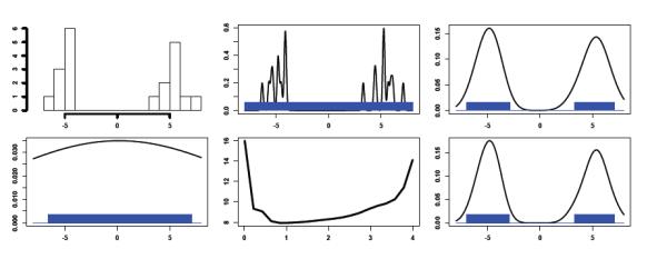
Top left: histogram of some data. Top middle, top right, and bottom left show three kernel density estimators and the corresponding conformal prediction sets with bandwidth 0.1, 1, and 10. Bottom middle: Lebesgue measure as a function of bandwidth. Bottom right: estimator and prediction set obtained from the bandwidth with smallest prediction set.

3.2 An approximation

The conformal prediction set is expensive to compute since we have to compute π_n(y) for every y ∈ ℝ^d. Here we derive an approximation to ${\widehat{C}}^{\left(\alpha \right)}$ that can be computed quickly and maintains finite sample validity. Define the upper and lower level sets of density p at level t, respectively:

$$Lt=\{y:p\left(y\right)\ge t\},\text{and}{L}^{\ell }\left(t\right)=\{y:p\left(y\right)\le t\}.$$ (8)

The corresponding level sets of ${\widehat{p}}_n$ are denoted L_n(t) and $L_n^l\left(t\right)$, respectively. Let Y₍₁₎, … , Y_(n) be the reordered data so that ${\widehat{p}}_n\left(Y_{\left(1\right)}\right)\le \cdots \le {\widehat{p}}_n\left(Y_{\left(n\right)}\right)$, and define the inner and outer sandwiching sets:

$$L_n^{-}=L_n\left({\widehat{p}}_n\left(Y_{\left(i_{n,\alpha }\right)}\right)\right),L_n^{+}=L_n\left({\widehat{p}}_n\left(Y_{\left(i_{n,\alpha }\right)}\right)-{\left({\mathit{nh}}^d\right)}^{-1}\psi K\right)$$

where ψ_K = sup_u,u′ |K(u) − K(u′)|. Then we have the following “sandwich” lemma, whose prrof can be found in Appendix B.

Lemma 3.1 (Sandwich Lemma). Let ${\widehat{C}}^{\left(\alpha \right)}$ be the conformal prediction set based on the kernel density estimator. Assume that sup_u |K(u)| = K(0). Then

$$L_n^{-}\subseteq {\widehat{C}}^{\left(\alpha \right)}\subseteq L_n^{+}.$$ (9)

According to the sandwich lemma, $L_n^{+}$ also guarantees distribution free finite sample coverage and is easier to analyze. Moreover, it is much faster to compute since it avoids ever having to compute the kernel density estimator based on the augmented data. The inner set, $L_n^{-}$, which is used as an estimate of C^(α) in related work such as in Chatterjee & Patra (1980); Hyndman (1996); Cadre et al. (2009), generally does not have finite sample validity. We confirm this through simulations in Section 5. Next we investigate the efficiency of these prediction sets.

3.3 Asymptotic properties

The inner and outer sandwiching sets $L_n^{-}$ and $L_n^{+}$ are plug-in estimators of density level sets of the form: $L_n\left(t_n^{\left(\alpha \right)}\right)=\{y:{\widehat{p}}_n\left(y\right)\ge t_n^{\left(\alpha \right)}\}$, where $t_n^{\left(\alpha \right)}={\widehat{p}}_n\left(Y_{\left(i_{n,\alpha }\right)}\right)$ for the inner set $L_n^{-}$ and $t_n^{\left(\alpha \right)}={\widehat{p}}_n\left(Y_{\left(i_{n,\alpha }\right)}\right)-{\left(n{h}_n^d\right)}^{-1}\psi K$ for the outer set $L_n^{+}$. Here we can view $t_n^{\left(\alpha \right)}$ as an estimate of t(α). In Cadre et al. (2009) it is shown that, under regularity conditions of the density p, the plug-in estimators $t_n^{\left(\alpha \right)}$ and L_n($t_n^{\left(\alpha \right)}$) are consistent with convergence rate $1∕\sqrt{n{h}_n^d}$ for a range of h_n. Here we refine the results under more general conditions. We note that similar convergence rates for plug-in density level sets with a fixed and known level are obtained in Rigollet & Vert (2009). The extension to unknown levels is nontrivial and needs slightly stronger regularity conditions.

Intuitively speaking, the plug-in density level set L_n($t_n^{\left(\alpha \right)}$) is an accurate estimator of L(t^(α)) if ${\widehat{p}}_n$ and $t_n^{\left(\alpha \right)}$ are accurate estimators of p and t^(α), and p is not too flat at level t^(α). The following smoothness condition is assumed for p and K to ensure accurate density estimation.

A1. The density p is Hölder smooth of order β, with β > 0, and K is a valid kernel of order β. Hölder smoothness and valid kernels are standard assumptions for nonparametric density estimation. We give their definitions in Appendix A.

Remark: Assumption A1 can be relaxed in a similar way as in Rigollet & Vert (2009). The idea is that we only need to estimate the density very accurately in a neighborhood of ∂C^(α) (the boundary of the optimal set). Therefore, it would be sufficient to have the strong β′-Hölder smoothness condition near ∂C^(α), together with a weaker β′-Hölder smoothness condition (β^t ≤ β) everywhere else. For presentation simplicity, we stick with the global smoothness condition in A1.

To control the regularity of p at level t^(α), a common assumption is the γ-exponent condition, which was first introduced by Polonik (1995) and has been used by many others (see Tsybakov (1997) and Rigollet & Vert (2009) for example). In our argument, such an assumption is also related to estimating t^(α) itself. Specifically, we assume

A2. There exist constants 0 < c₁ ≤ c₂ and ∈₀ > 0 such that

$$c_1{\mid ∊\mid }^{\gamma }\le \mid P\left(\{y:p\left(y\right)\le t^{\left(\alpha \right)}+∊\}\right)-\alpha \mid \le c_2{\mid ∊\mid }^{\gamma },\forall -{∊}_0\le ∊\le {∊}_0.$$ (10)

The gamma exponent condition requires that the density to be neither flat (for stability of level set) nor steep (for accuracy of $t_n^{\left(\alpha \right)}$). As indicated in Audibert & Tsybakov (2007), A1 and A2 cannot hold simultaneously unless γ(1 ^ β) ≤ 1. In the common case γ = 1, this always holds.

Assumptions A1 and A2 extend those in Cadre et al. (2009), where β = γ = 1 is considered. The next theorem states the quality of cut-off values used in the sandwiching sets $L_n^{-}$ and $L_n^{+}$.

Theorem 3.2. Let $t_n^{\left(\alpha \right)}={\widehat{p}}_n\left(Y_{\left(i_{n,\alpha }\right)}\right)$, where ${\widehat{p}}_n$ is the kernel density estimator given by eq. (6), and Y_(i) and i_n,α are defined as in Section 3.2. Assume that A1-A2 hold and choose $h_n\asymp {(\log n∕n)}^{1∕(2\beta +d)}$. Then for any λ > 0, there exist constants A_λ, $A_{\lambda }^{\prime }$ depending only on p, K and α, such that

$$\mathbb{\mathbb{P}}\left(\mid t_n^{\left(\alpha \right)}-t^{\left(\alpha \right)}\mid \ge A_{\lambda }{\left(\frac{\log n}{n}\right)}^{\frac{\beta }{2\beta +d}}+A_{\lambda }^{\prime }{\left(\frac{\log n}{n}\right)}^{\frac{1}{2\gamma }}\right)=O\left(n^{-\lambda }\right).$$ (11)

We give the proof of Theorem 3.2 in Appendix C. Theorem 3.2 is useful for establishing the convergence of the corresponding level set. Observing that $\left(n{h}_n^d\right)=o\left({(\log n∕n)}^{\beta ∕(2\beta +d)}\right)$, it follows immediately that the cut-off value used in $L_n^{+}$ also satisfies (11). The next theorem, proved in Appendix C, gives the rate of convergence for our estimators.

Theorem 3.3. Under same conditions as in Theorem 3.2, for any λ > 0, there exist constants B_λ, $B_{\lambda }^{\prime }$ depending on p, K and α only, such that, for all $\widehat{C}∊\{{\widehat{C}}^{\left(\alpha \right)},L_n^{-},L_n^{+}\}$,

$$\mathbb{\mathbb{P}}\left(\mu (\widehat{C}\Delta C^{\left(\alpha \right)})\ge B_{\lambda }{\left(\frac{\log n}{n}\right)}^{\frac{\beta \gamma }{2\beta +d}}+B_{\lambda }^{\prime }{\left(\frac{\log n}{n}\right)}^{\frac{1}{2}}\right)=O\left(n^{-\lambda }\right).$$ (12)

Remark: In the most common cases γ = 1, or β ≥ 1/2, γβ ≤ 1, the term (log n/n)^βγ/(2β+d) dominates the convergence rate. It matches the minimax risk rate of the plug-in density level set at a known level developed by Rigollet & Vert (2009). As a result, not knowing the cut-off value t^(α) does not change the difficulty of estimation. When βγ/(2β + d) > 1/2, the rate is dominated by (log n/n)^1/2 and does not agree with the known minimax lower bound and we do not know if the $\sqrt{\log n∕n}$ can be eliminated from the result.

Remark: The theorems above were stated for the optimal choice of bandwidth. The method is still consistent with similar arguments whenever $n{h}_n^d∕\log n\to \infty$ and h_n → 0, although the resulting rates will no longer be optimal.

Remark: The same conclusions in Theorems 3.2 and 3.3 hold under a weaker version of Assumption A1. To make this idea more precise, suppose the density function is only β-Hölder smooth in a neighborhood of the level set contour {y : p(y) = t^(α)}, but less smooth everywhere else. Then the same proofs of Theorems 3.2 and 3.3 can be used to obtain a slower rate of convergence. After establishing this first consistency result, one can apply the argument again, with the analysis confined in the smooth neighborhood, to obtain the desired rate of convergence. However, in the interest of space and clarity, we will prove our results only under the more restrictive smoothness assumptions that we have stated.

Algorithm 1: Tuning With Sample Splitting.

Input: sample Y = (Y₁, …, Y_n), prediction set estimator $\widehat{C}$ level α, and candidate set H

1. Split the sample randomly into two equal sized subsamples, Y₁ and Y₂.

2. Construct prediction sets $\{{\widehat{C}}_{h,1}:h∊H\}$ each at level 1 − α, using subsample Y₁.

3. Let $\widehat{h}$ = arg min_h μ(${\widehat{C}}_{h,1}$).

4. 4. Return ${\widehat{C}}_{\widehat{h},2}$, which is constructed using bandwidth $\widehat{h}$ and subsample Y₂.

4. CHOOSING THE BANDWIDTH

As illustrated in Figure 1, the efficiency of ${\widehat{C}}^{\left(\alpha \right)}$ depends on the choice of h_n. The size of estimated prediction sets can be very large if the bandwidth is either too large or too small. Therefore, in practice it is desirable to choose a good bandwidth in an automatic and data driven manner. In kernel density estimation, the choice of bandwidth has been one of the most important topics and many approaches have been studied; see Loader (1999), Mammen, Miranda, Nielsen & Sperlich (2011), Samworth & Wand (2010) and references therein. Here we consider choosing the bandwidth by minimizing the volume of the conformal prediction set.

Let H = {h₁, … , h_m} be a grid of candidate bandwidths. We compute the prediction set for each h ∈ H and choose the one with the smallest volume. To preserve finite sample validity, we use sample splitting as described in Algorithm 1. We state the following result and omit its proof.

Proposition 4.1. If$\widehat{C}$ satisfies finite sample validity for all h, then ${\widehat{C}}_{\widehat{h},2}$, the output of the sample splitting tuning algorithm, also satisfies finite sample validity.

There are two justifications for choosing a bandwidth to make $\mu \left({\widehat{C}}_h\right)$ small. The first is pragmatic: in making predictions it seems desirable to have a small prediction set. The second reason is that minimizing μ(C) can potentially lead to good risk properties in terms of the loss μ(CΔC^(α)) as we now show. Recall that R(C) = μ(CΔC^(α)) and define ε(C) = μ(C) − μ(C^(α)). To avoid technical complications, we will assume in this section that the sample space is compact and focus on the simple case γ = 1 in condition A2.

Lemma 4.2. Let $\widehat{C}$ be an estimator of C^(α). Then $\epsilon \left(\widehat{C}\right)\le R\left(\widehat{C}\right)$ Furthermore, if $\widehat{C}$ is finite sample valid and A2 holds with γ = 1, then $\mathbb{𝔼}\left(R\left(\widehat{C}\right)\right)\le c_1{\left[\mathbb{𝔼}\left(\epsilon \left(\widehat{C}\right)\right)\right]}^{1∕2}$ for some constant c₁.

The bandwidth selection algorithm makes $\epsilon \left(\widehat{C}\right)$ small. The lemma gives at least us some assurance that making $\epsilon \left(\widehat{C}\right)$ small will help to make $R\left(\widehat{C}\right)$ small. The proof of Lemma 4.2 is given in Appendix D. (A similar result can be found in Scott & Nowak (2006).) However, it is an open question whether $R\left(\widehat{C}\right)$ achieves the minimax rate.

5. NUMERICAL EXAMPLES

We first consider simulations on Gaussian mixtures and double-exponential mixtures in two and three dimensions. We apply the bandwidth selector presented in Section 4 to both ${\widehat{C}}^{\left(\alpha \right)}$ and $L_n^{+}$. The bandwidth used for $L_n^{-}$ is the same as that for $L_n^{+}$. Therefore, in the results it is possible to see if $L_n^{-}$ is bigger than ${\widehat{C}}^{\left(\alpha \right)}$, or if ${\widehat{C}}^{\left(\alpha \right)}$ is bigger than $L_n^{-}$ because of different bandwidths and data splitting.

5.1 2D Gaussian mixture

We first consider a two-component Gaussian mixture in ℝ². The first component has mean ($\sqrt{2\log n}-2,0$) and variance diag(4, 1/4), and the second component has mean (0, $\sqrt{2\log n}-2$) and variance diag(1/4, 4) (see Figure 2). This choice of component centers is to make a moderate overlap between the data clouds from the two components. It makes the prediction set problem more challenging.

Figure 2.

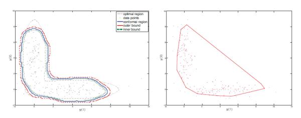
Conformal prediction set (left) and the convex hull of the multivariate spacing depth based tolerance set (right), with data from a two-component Gaussian mixture.

Table 1 shows the coverage and Lebesgue measure of the prediction set at level 0.9 (α = 0.1) over 100 repetitions. The coverage is excellent and the size of the set is close to optimal. Both the conformal set ${\widehat{C}}^{\left(\alpha \right)}$ and the outer sandwiching set $L_n^{+}$ give correct coverage regardless of the sample size. It is worth noting that the inner sandwiching set $L_n^{-}$ (corresponding to the method in Hyndman (1996); Park et al. (2010)) does not give the desired coverage, which suggests that decreasing the cut-off value in $L_n^{+}$ is not merely an artifact of proof, but a necessary tuning. The observed excess loss also reflects a rate of convergence that supports our theoretical results on the symmetric difference loss. We compare our method with the approach introduced by Zhao & Saligrama (2009) (Ĉ_ZS), where the prediction set is constructed by ranking the distances from each data point to its kth nearest neighbor. It has been reported that the choice of k is not crucial and we use k = 6. (We remark further on the choice of k at the end of this section.) This method is similar to ours but does not have finite sample validity. We observe that the finite sample coverage Ĉ_ZS is less than the nominal level.

Table 1.

The simulation results for 2-d Gaussian mixture with α = 0.1 over 100 repetitions (mean and one standard deviation). The Lebesgue measure of the ideal set ≈ 28.02.

		Coverage		Lebesgue Measure
	n = 100	n = 200	n = 1000	n = 100	n = 200	n = 1000
${\widehat{C}}^{\left(\alpha \right)}$	0.886 ± 0.005	0.897 ± 0.002	0.900 ± 0.001	35.6 ± 0.7	34.3 ± 0.3	31.1 ± 0.2
$L_n^{-}$	0.861 ± 0.004	0.882 ± 0.001	0.896 ± 0.001	29.8 ± 0.3	34.1 ± 0.2	32.2 ± 0.1
$L_n^{+}$	0.907 ± 0.003	0.900 ± 0.001	0.907 ± 0.001	36.2 ± 0.4	36.9 ± 0.2	34.1 ± 0.1
${\widehat{C}}^{\mathrm{ZS}}$	0.853 ± 0.004	0.867 ± 0.002	0.881 ± 0.001	28.1 ± 0.4	28.2 ± 0.2	28.0 ± 0.1

Figure 2 shows a typical realization of the estimators. In both panels, the dots are data points when n = 200. The left panel shows the conformal prediction set with sample splitting (blue solid curve), together with the inner and outer sandwiching sets (red dashed and green dotted curves, respectively). Also plotted is the ideal set C^(α) (grey dash-dotted curve). It is clear that all three estimated sets capture the main part of the ideal set, and they are mutually close. On the right panel we plot a realization of the depth based approach from Li & Liu (2008). This approach does not require any tuning parameter. However, it takes O(n^d+1) time to evaluate 1(y ∈ Ĉ) for any single y. In practice it is recommended to compute the empirical depth only for all the data points and use the convex hull of all data points with high depth as the estimated prediction set. Such a convex hull construction misses the “L” shape of the ideal set. Moreover, in our implementation the running time of the kernel density method is much shorter even when n = 200.

Figure 3 shows the effect of bandwidth on the excess loss ε(Ĉ) = μ(Ĉ) − μ(Ĉ)^(α)) based on a typical implementation with n = 200, where the y axis is the Lebesgue measure of the estimated sets. We observe that for the conformal prediction set Ĉ^(α), the excess loss is stable for a wide range of bandwidths, especially that moderate undersmoothing does not harm the performance very much. An intuitive explanation is that the data near the contour are dense enough to allow for moderate undersmoothing. Similar phenomenon should be expected whenever α is not too small. Moreover, the selected bandwidth from the outer sandwiching set $L_n^{+}$ is close to that obtained from the conformal set. This observation may be of practical interest since it is usually much faster to compute $L_n^{+}$.

Figure 3.

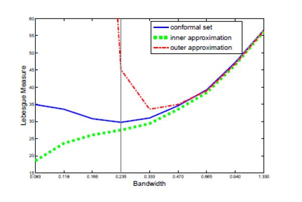
Lebesgue measure of prediction sets versus bandwidth.

Remark: The Ĉ^ZS method requires a choice of k. We tried k = 2, 3, … , 20. The coverage increases with k but does not reach the nominal 0.9 level even when k = 20. The Lebesgue measure also increases with k and after k = 20, it becomes larger than the conformal region.

5.2 Further simulations

We now investigate the performance of our method using distributions with heavier tails and in higher dimensions. These simulations confirm that our method always give finite sample coverage, even when the density estimation is very challenging.

Double exponential distribution

In this setting, the distribution also has two balanced components. The first component has independent double exponential coordinates: Y (1) ~ 2 DoubleExp(1)+2.2 log n, Y(2) ~ 0.5 DoubleExp(1), where DoubleExp(1) has density exp(−|y|)/2. The second component has the two coordinates switched. The centering at 2.2 log n is chosen so that there is moderate overlap between data clouds from two components. The results are summarized in Table 2.

Table 2.

The simulation results for 2-d double exponential mixture with α = 0.1 over 100 repetitions (mean and one standard deviation). The Lebesgue measure of the ideal set ≈ 55.

		Coverage		Lebesgue Measure
	n = 100	n = 200	n = 1000	n = 100	n = 200	n = 1000
${\widehat{C}}^{\left(\alpha \right)}$	0.895 ± 0.005	0.916 ± 0.003	0.91 ± 0.002	77.7 ± 3	76.6 ± 1.6	62.3 ± 0.6
$L_n^{-}$	0.864 ± 0.006	0.897 ± 0.003	0.90 ± 0.001	66.5 ± 2.3	71.7 ± 1.2	58.3 ± 0.3
$L_n^{+}$	0.893 ± 0.005	0.912 ± 0.003	0.92 ± 0.001	86.1 ± 7.4	78.2 ± 1.3	65.0 ± 0.4
${\widehat{C}}^{\mathrm{ZS}}$	0.871 ± 0.004	0.892 ± 0.003	0.897 ± 0.001	58.2 ± 1.5	60.2 ± 1.0	55.2 ± 0.4

Three-dimensional data

Now we increase the dimension of data. The Gaussian mixture is the same as in the 2-dimensional setup, with the third coordinate being an independent Gaussian with mean zero and variance 1/4. The results are summarized in Table 3.

Table 3.

The simulation results for 3-d Gaussian mixture with α = 0.1 over 100 repetitions (mean and one standard deviation). The Lebesgue measure of the ideal set ≈ 62.

		Coverage		Lebesgue Measure
	n = 100	n = 200	n = 1000	n = 100	n = 200	n = 1000
${\widehat{C}}^{\left(\alpha \right)}$	0.917 ± 0.004	0.902 ± 0.003	0.900 ± 0.002	109 ± 2.4	89 ± 1.5	74 ± 0.7
$L_n^{-}$	0.875 ± 0.005	0.880 ± 0.003	0.889 ± 0.002	109 ± 2.1	98 ± 1.5	81 ± 0.7
$L_n^{+}$	0.892 ± 0.004	0.898 ± 0.003	0.916 ± 0.002	118 ± 2.2	109 ± 1.6	96 ± 0.9
${\widehat{C}}^{\mathrm{ZS}}$	0.869 ± 0.003	0.872 ± 0.002	0.879 ± 0.001	75 ± 1.3	69 ± 0.8	64 ± 0.4

Remark: In the above two simulation settings, the conformal prediction sets are much larger than the ideal (oracle) set unless the sample size is very large (n = 1000). This is because of the difficulty of multivariate nonparametric density estimation. In fact, the kernel density estimator may no longer lead to a good conformity score in this case. However, the theory of conformal prediction is still valid as reflected by the coverage. Thus, one may use other conformity scores such as the k-nearest-neighbor radius, for which a non-conformal version has been reported in Zhao & Saligrama (2009). Other possible choices include Gaussian mixture density estimators and semi-parametric models. These extensions will be pursued in future work.

5.3 Application to Breast Cancer Data

In this subsection we apply our method to the Wisconsin Breast Cancer Dataset (available at the UCI machine learning repository). The data contains nine features of 699 patients among which 241 are malignant and 458 are benign. Although this data set is commonly used to test classification algorithms, it has been used to test prediction region methods in the literature (see Park et al. (2010) for example). In this example we use prediction sets to tell malignant cases from benign ones. Formally, we assume that the benign cases are sampled from a common distribution, and we construct a 95% prediction set corresponding to the high density region of the underlying distribution. Although the prediction sets are constructed using only the benign cases, the efficiency of the estimated prediction/tolerance set can be measured not only in terms of its Lebesgue measure, but also in terms of the number of false negatives (i.e., the number of malignant cases covered by the prediction set). Ideally the prediction set shall contain most of benign cases but few malignant cases and hence can be used as a classifier.

In our implementation, the data dimension is reduced to two using standard principal components analysis. Such a dimension reduction simplifies visualization and has also been used in Park et al. (2010). If no dimension reduction is used, the data concentrates near a low dimensional subset of the space, and other conformity scores, such as the k nearest neighbors radius, can be used instead of kernel density estimation. To test the out of sample performance of our method, we randomly choose 100 out of 458 benign cases as testing data. The prediction region is constructed using only the remaining 358 benign cases with coverage level 0.95 and kernel density bandwidth 0.8. We repeat this experiment 100 times. A typical implementation is plotted in Figure 4. In Table 4 we report the mean coverage on the testing data as well as the malignant data. The resulting conformal prediction sets give the desired coverage for the benign cases and low false coverage for the malignant cases. Note that in this case the inner density level set $L_n^{-}$ is equivalent to the method proposed in Park et al. (2010), which in general does not have finite sample validity. In our experiment, the average out-of-sample coverage is slightly below the nominal level (by about one standard deviation). In this example, we see that the conformal methods (Ĉ^(α) and $L_n^{+}$) give similar empirical performance as the conventional non-conformal method ($L_n^{-}$), with additional finite sample guarantee.

Figure 4.

Prediction sets for benign instances. Crosses: benign; diamonds: malignant. Blue dashed curve: $L_n^{+}$; Black dotted curve: $L_n^{-}$; Red solid curve: Ĉ^(α).

Table 4.

Application to the breast cancer data with α = 0.05 over 100 repetitions. Reported are the mean and one estimated standard deviation of the empirical coverage on the testing benign data and the malignant data.

method	${\widehat{C}}^{\left(\alpha \right)}$	$L_n^{-}$	$L_n^{+}$
test sample coverage	0.9514 ± 0.0012	0.9488 ± 0.0012	0.9534 ± 0.0013
malignant data coverage	0.0141 ± 0.0002	0.0044 ± 0.0001	0.0420 ± 0.0004

APPENDIX A. DEFINITIONS

A.1 Hölder smooth functions

The Hölder class is a popular smoothness condition in nonparametric inferences (Tsybakov 2009, Section 1.2). Here we use the version given in (Rigollet & Vert 2009).

Let s = (s₁, …, s_d) be a d-tuple of non-negative integers and |s| = s₁ + … + s_d. For any x ∈ ℝ^d, let $x^s=x_1^{S_1}\cdots x_d^{S_d}$ and D^s be the differential operator:

$$D^{s}f=\frac{{\partial }^{\mid s\mid }f}{\partial x_1^{s_1}\cdots \partial x_d^{s_d}}(x_1,\dots ,x_d).$$

Given β > 0, for any functions f that are [β] times differentiable, denote its Taylor expansion of

degree [βJ at x₀ by

$$f_{x_0}^{\left(\beta \right)}\left(x\right)=\sum _{\mid s\mid \le \beta }\frac{{(x-x_0)}^s}{s_1!\cdots s_d!}{D}^{s}f\left(x_0\right).$$

Definition A.1 (Hölder class). For constants β > 0, L > 0, define the Hölder class Σ(β, L) to be the set of lβJ-times differentiable functions on ℝ^d such that,

$$\mid f\left(x\right)-f_{x_0}^{\left(\beta \right)}\left(x\right)\mid \le L{\parallel x-x_0\parallel }^{\beta }.$$ (A.1)

A.2 Valid kernels

A standard condition on the kernel is the notion of β-valid kernels.

Definition A.2 (β-valid kernel). For any β > 0, function K : ℝ^d → ℝ¹ is a β-valid kernel if (a) K is supported on [−1, 1]^d; (b) ∫ K = 1; (c) ∫ |K|^r < ∞, all r ≥ 1; (d) ∫ y^sK(y)dy = 0 for all 1 ≤ |s| ≤ β.

The last condition is interpreted elementwise. In the literature, β-valid kernels are usually used with Hölder class of functions to derive fast rates of convergence. The existence of univariate β-valid kernels can be found in Section 1.2 of Tsybakov (2009). A multivariate β-valid kernel can be obtained by taking direct product of univariate β-valid kernels.

APPENDIX B. PROOF OF LEMMA 3.2

Proof Lemma 3.1. Let $P_n^y=\frac{n}{n+1}{P}_n+\frac{1}{n+1}{\delta }_y$, where P_n is the empirical distribution defined by the sample Y = (Y₁, …, Y_n), and δ_y is the point mass distribution at y. Define functions

$$\begin{array}{cc}\hfill G\left(t\right)& =P\left(L^{\ell }\left(t\right)\right),\hfill \\ \hfill G_n\left(t\right)& =P_n\left(L_n^{\ell }\left(t\right)\right)=n^{-1}\sum _{i=1}^{n}1({\widehat{p}}_n\left(Y_i\right)\le t),\hfill \\ \hfill G_n^y\left(t\right)& =P_n^y({\widehat{p}}_n^y\left(Y\right)\le t)=\frac{1}{n+1}\left(\sum _{i=1}^{n}1({\widehat{p}}_n^y\left(Y_i\right)\le t)+1({\widehat{p}}_n^y\left(y\right)\le t)\right).\hfill \end{array}$$

The functions G, G_n and $G_n^y$ defined above are the cumulative distribution function (CDF) of p(Y ) and its empirical versions with sample Y and aug(Y, y), respectively, where aug(Y, y) = (Y₁, … , Y_n, y). By (5) and Algorithm 1, the conformal prediction set can be written as

$${\widehat{C}}^{\left(\alpha \right)}=\left\{y\in {\mathbb{ℝ}}^d:G_n^y\left({\widehat{p}}_n^y\left(y\right)\right)\ge \tilde{\alpha }\right\}.$$

The proof is based on a direct characterization of $L_n^{-}$ and $L_n^{+}$. First, for each y ∈ $L_n^{-}$ and i ≤ i_n,α, we have

$${\widehat{p}}_n^y\left(y\right)-{\widehat{p}}_n^y\left(Y_{\left(i\right)}\right)=\frac{n}{n+1}({\widehat{p}}_n\left(y\right)-{\widehat{p}}_n\left(Y_{\left(i\right)}\right))+\frac{1}{(n+1)h^d}\left(K\left(0\right)-K\left(\frac{Y_{\left(i\right)}-y}{h}\right)\right)\ge 0.$$

As a result, $G_n^y\left({\widehat{p}}_n^y\left(y\right)\right)\le i_{n,\alpha }∕(n+1)=\tilde{\alpha }$ and hence y ∈ Ĉ^(α). Similarly, for each y ∈ $L_n^{+}$ and i ≥ i_n,α we have

$$\begin{array}{cc}\hfill {\widehat{p}}_h^y\left(y\right)-{\widehat{p}}_h^y\left(Y_{\left(i\right)}\right)& =\frac{n}{n+1}({\widehat{p}}_h\left(y\right)-{\widehat{p}}_h\left(Y_{\left(i\right)}\right))+\frac{1}{(n+1)h^d}\left(K\left(0\right)-K\left(\frac{Y_{\left(i\right)}-y}{h}\right)\right)\hfill \\ \hfill & \le \frac{n}{n+1}({\widehat{p}}_h\left(y\right)-{\widehat{p}}_h\left(Y_{\left(i_{n,\alpha }\right)}\right))+\frac{1}{(n+1)h^d}{\psi }_K<0.\hfill \end{array}$$

Therefore, $G_n^y\left({\widehat{p}}_n^y\left(y\right)\right)\le \left(i_{n,\alpha 1}\right)∕(n-1)=\tilde{\alpha }$ and hence y ∈ Ĉ^(α).

APPENDIX C. PROOF OF THEOREM 3.3

The bias in the estimated cut-off level $t_n^{\left(\alpha \right)}$ can be bounded in terms of two quantities:

$$V_n=\underset{t>0}{\sup }\mid P_n\left(L^{\ell }\left(t\right)\right)-P\left(L^{\ell }\left(t\right)\right)\mid ,R_n={\parallel {\widehat{p}}_n-p\parallel }_{\infty }.$$

Here V_n can be viewed as the maximum of the empirical process P_n − P over a nested class of sets, and R_n is the L_∞ loss of the density estimator. As a result, V_n can be bounded using the standard empirical process and VC dimension argument, and R_n can be bounded using the smoothness of p and kernel K with a suitable choice of bandwidth. Formally, we provide upper bounds for these two quantities through the following lemma.

Lemma C.1. Let V_n, R_n be defined as above, then under Assumptions A1 and A2, for any λ > 0, there exist constants A_1,λ and A_2,λ depending on λ only, such that,

$$\mathbb{\mathbb{P}}\left(V_n\ge A_{1,\lambda }\sqrt[]{\frac{\log n}{n}}\right)=O\left(n^{-\lambda }\right),\mathbb{\mathbb{P}}\left(R_n\ge A_{2,\lambda }{\left(\frac{\log n}{n}\right)}^{\frac{\beta }{2\beta +d}}\right)=O\left(n^{-\lambda }\right).$$

Proof. First, it is easy to check that the class of sets {L^f(t) : t > 0} are nested with VC (Vapnik-Chervonenkis) dimension 2 and hence by classical empirical process theory (see, for example, van der Vaart & Wellner (1996), Section 2.14) , there exists a constant C₀ > 0 such that for all η > 0

$$\mathbb{\mathbb{P}}(V_n\ge \eta )\le C_0{n}^2\exp (-n{\eta }^2∕32).$$ (A.2)

Let η = $A\sqrt{\log n∕n}$, we have

$$\mathbb{\mathbb{P}}(V_n\ge A\sqrt[]{\log n∕n})\le C_0{n}^2\exp (-A^2\log n∕32)=C_0{n}^{-(A^2∕32-2)}.$$ (A.3)

The first result then follows by choosing $A_{1,\lambda }=\sqrt{32(\lambda +2)}$. Next we bound R_n. Let p̄ = 𝔼[p̂_n], and ∈_n = (log n/n)^β/(2β+d). By triangle inequality R_n ≤ || p̂_n − p̄||∞ + ||p̄ − p||_∞. Due to a result of Giné & Guillou (2002) (see also (49) in Chapter 3 of Prakasa Rao (1983)), under Assumption A1, there exist constants C₁, C₂ and B₀ > 0 such that have for all B ≥ B₀,

$$\mathbb{\mathbb{P}}({\parallel {\widehat{p}}_n-\stackrel{‒}{p}\parallel }_{\infty }\ge B{∊}_n)\le C_1\exp (-C_2{B}^2\log \left(h_n^{-1}\right))=C_1{h}_n^{C_2{B}^2}.$$ (A.4)

On the other hand, by Assumption A1, for some constant C₃

$${\parallel \stackrel{‒}{p}-p\parallel }_{\infty }\le C_3{h}_n^{\beta }.$$ (A.5)

In (A.3), (A.4) and (A.5) the constants C_i, i = 0, …, 3, depend on p and K only. Hence,

$$\mathbb{\mathbb{P}}({\parallel \widehat{p}-\stackrel{‒}{p}\parallel }_{\infty }\ge (C_3+B){∊}_n)\le C_1{h}_n^{C_2{B}^2},$$ (A.6)

which concludes the second part by choosing $A_{2,\lambda }=C_3+\sqrt{\frac{(2\beta +d)\lambda }{C_2}}$. □

Proof of Theorem 3.2. Let α_n = i_n,α/n = l(n + 1)αJ/n. We have |α_n − α| ≤ 1/n. Recall that the ideal level t^(α) can be written as t^(α) = G⁻¹(α) where the function G is the cumulative distribution function of p(Y ), as defined in Subsection 3.2. By the γ-exponent condition the inverse of G is well defined in a small neighborhood of α. When n is large enough, we can define t^(αn) as t^(αn) = G⁻¹(α_n).

Again, by the γ-exponent condition, $c_1\mid t^{\left({\alpha }_n\right)}-t^{\left(\alpha \right)}{\mid }^{\gamma }\le \mid G\left(t^{\left({\alpha }_n\right)}\right)-G\left(t^{\left(\alpha \right)}\right)\mid =\mid {\alpha }_n-\alpha \le \frac{1}{n}$. Therefore, for n large enough

$$\mid t^{\left({\alpha }_n\right)}-t^{\left(\alpha \right)}\mid \le {\left(c_{1}n\right)}^{-1∕\gamma }.$$ (A.7)

Equation (A.7) allows us to switch to the problem of bounding $\mid t_n^{\left(\alpha \right)}-t^{\left({\alpha }_n\right)}\mid$. Recall that $t_n^{\left(\alpha \right)}={\widehat{p}}_n\left(Y_{\left(i_{n,\alpha }\right)}\right)$. The key of the proof is to observe that $t_n^{\left(\alpha \right)}=G_n^{-1}\left({\alpha }_n\right):=\inf \{t:G_n\left(t\right)\ge {\alpha }_n\}$. Then it suffices to show that G⁻¹ and G⁻¹ are close at α_n. In fact, by definition of R_n we have for all $tq0:L^l(t-R_n)\subseteq L_n^l\left(t\right)\subseteq L^l(t+R_n)$. As a result, we have

$$P_n\left(L^{\ell }(t-R_n)\right)\le P_n\left(L_n^{\ell }\left(t\right)\right)\le P_n\left(L^{\ell }(t+R_n)\right).$$

By definition of V_n,

$$P\left(L^{\ell }(t-R_n)\right)-V_n\le P_n\left(L_n^{\ell }\left(t\right)\right)\le P\left(L^{\ell }(t+R_n)\right)+V_n.$$

By definition of G and G_n, the above inequality becomes

$$G(t-R_n)-V_n\le G_n\left(t\right)\le G(t+R_n)+V_n.$$

Let W_n = R_n + (2V_n/c₁)^1/γ . Suppose n is large enough such that

$${\left(\frac{c_1}{n}\right)}^{\frac{1}{\gamma }}+{\left(\frac{2A_{1,\lambda }}{c_1}\sqrt[]{\frac{\log n}{n}}\right)}^{\frac{1}{\gamma }}<{∊}_0,$$

then on the event $V_n\le A_{1,\lambda }\sqrt{\frac{\log n}{n}}$,

$$\begin{array}{cc}\hfill G_n\left(t^{\left({\alpha }_n\right)}-W_n\right)& \le G\left(t^{\left({\alpha }_n\right)}-W_n+R_n\right)+V_n\hfill \\ \hfill & =G\left(t^{\left({\alpha }_n\right)}-{(2V_n∕c_1)}^{1∕\gamma }\right)-G\left(t^{\left({\alpha }_n\right)}\right)+{\alpha }_n+V_n\hfill \\ \hfill & \le {\alpha }_n-V_n<{\alpha }_n.\hfill \end{array}$$

where the last inequality uses the left side of the γ-exponent condition. Similarly, G_n(t^(αn) + W_n) > α_n. Hence, for n large enough, if $V_n\le A_{1,\lambda }\sqrt{\left(\log n\right)∕n}$ then,

$$\mid t_n^{\left(\alpha \right)}-t^{\left({\alpha }_n\right)}\mid \le W_n.$$ (A.8)

To conclude the proof, first note that ${\left(\frac{c_1}{n}\right)}^{\frac{1}{\gamma }}=o\left({\left(\frac{\log n}{n}\right)}^{\frac{1}{2\gamma }}\right)$. Then we can find constant $A_{\lambda }^{\prime }$ such that for all n large enough,

$$\left(A_{\lambda }^{\prime }-{\left(\frac{2A_{1,\lambda }}{c_1}\right)}^{\frac{1}{\gamma }}\right){\left(\frac{\log n}{n}\right)}^{\frac{1}{2\gamma }}\ge {\left(\frac{c_1}{n}\right)}^{\frac{1}{\gamma }}.$$ (A.9)

Let A_λ = A_2,λ. Combining equations (A.7) and (A.8), on the event

$$E_{n,\lambda }≔\left\{R_n\le A_{\lambda }{\left(\frac{\log n}{n}\right)}^{\frac{\beta }{2\beta +d}},V_n\le A_{1,\lambda }{\left(\frac{\log n}{n}\right)}^{\frac{1}{2}}\right\},$$ (A.10)

we have, for n large enough,

$$\begin{array}{cc}\hfill \mid t_n^{\left(\alpha \right)}-t^{\left(\alpha \right)}\mid & \le \mid t_n^{\left(\alpha \right)}-t^{\left({\alpha }_n\right)}\mid +{\left(\frac{c_1}{n}\right)}^{\frac{1}{\gamma }}\le W_n+{\left(\frac{c_1}{n}\right)}^{\frac{1}{\gamma }}\hfill \\ \hfill & \le R_n+\left(2c_{c_1}^{-1}{V_n}^{1∕\gamma }\right)+{\left(\frac{c_1}{n}\right)}^{\frac{1}{\gamma }}\hfill \\ \hfill & \le A_{\lambda }{\left(\frac{\log n}{n}\right)}^{\frac{\beta }{2\beta +d}}+{\left(\frac{2A_{1,\lambda }}{c_1}\sqrt[]{\frac{\log n}{n}}\right)}^{\frac{1}{\gamma }}+{\left(\frac{c_1}{n}\right)}^{\frac{1}{\gamma }}\hfill \\ \hfill & \le A_{\lambda }{\left(\frac{\log n}{n}\right)}^{\frac{\beta }{2\beta +d}}+A_{\lambda }^{\prime }{\left(\frac{\log n}{n}\right)}^{\frac{1}{2\gamma }}\hfill \end{array}$$

where the second last inequality is from the definition of E_n,λ and the last inequality is from the choice of $A_{\lambda }^{\prime }$. The proof is concluded by observing $\mathbb{\mathbb{P}}\left(E_{n,\lambda }^c\right)=O\left(n^{-\lambda }\right)$, a consequence of Lemma C.1. □

Proof of Theorem 3.3. In the proof we write t_n for $\mathbb{\mathbb{P}}\left(E_{n,\lambda }^c\right)=O\left(n^{-\lambda }\right)$ as a generic estimate of t^(α) that satisfies (11). Observe that

$$\mu \left(L_n\left(t_n\right)\Delta C^{\left(\alpha \right)}\right)=\mu \left(\left\{{\widehat{p}}_n\ge t_n,p<t^{\left(\alpha \right)}\right\}\right)+\mu \left(\left\{{\widehat{p}}_n<t_n,p\ge t^{\left(\alpha \right)}\right\}\right).$$ (A.11)

Note that

$$\left\{{\widehat{p}}_n\ge t_n,p<t^{\left(\alpha \right)}\right\}\subseteq \left\{t^{\left(\alpha \right)}-\mid t_n-t^{\left(\alpha \right)}\mid -R_n\le p<t^{\left(\alpha \right)}\right\},$$ (A.12)

and Therefore

$$\left\{{\widehat{p}}_n<t_n,p\ge t^{\left(\alpha \right)}\right\}\subseteq \left\{t^{\left(\alpha \right)}<p\le t^{\left(\alpha \right)}+\mid t^{\left(\alpha \right)}-t_n\mid +R_n\right\}.$$ (A.13)

Suppose n is large enough such that

$$L_n\left(t_n\right)\Delta C^{\left(\alpha \right)}\subseteq \left\{t^{\left(\alpha \right)}-\mid t_n-t^{\left(\alpha \right)}\mid -R_n<p\le t^{\left(\alpha \right)}+\mid t^{\left(\alpha \right)}-t_n\mid +R_n\right\}.$$ (A.14)

Suppose n is large enough such that

$$2A_{2,\lambda }{\left(\frac{\log n}{n}\right)}^{\frac{\beta }{2\beta +d}}+A_{\lambda }^{\prime }{\left(\frac{\log n}{n}\right)}^{\frac{1}{2\gamma }}<\left({∊}_0\wedge \frac{t^{\left(\alpha \right)}}{2}\right),$$

where the constant A_2,λ is defined as in Lemma C.1 and $A_{\lambda }^{\prime }$ is defined as in equation (A.9). Then on the event E_n,λ as defined in equation (A.10), applying Theorem 3.2 and condition (10) on the right hand side of (A.14) yields

$$\begin{array}{cc}\hfill \mu \left(L_n\left(t_n\right)\Delta C^{\left(\alpha \right)}\right)& \le \frac{P\left(L_n\left(t_n\right)\Delta C^{\left(\alpha \right)}\right)}{t^{\left(\alpha \right)}-\mid t_n-t^{\left(\alpha \right)}\mid -R_n}\hfill \\ \hfill & \le \frac{2}{t^{\left(\alpha \right)}}{c}_2{\left(2A_{2,\lambda }{\left(\frac{\log n}{n}\right)}^{\frac{\beta }{2\beta +d}}+A_{\lambda }^{\prime }{\left(\frac{\log n}{n}\right)}^{\frac{1}{2\gamma }}\right)}^{\gamma }\hfill \\ \hfill & \le B_{\lambda }{\left(\frac{\log n}{n}\right)}^{\frac{\beta \gamma }{2\beta +d}}+B_{\lambda }^{\prime }{\left(\frac{\log n}{n}\right)}^{\frac{1}{2}},\hfill \end{array}$$ (A.15)

where B_λ, $B_{\lambda }^{\prime }$ are positive constants depending only on p, K, α and γ. As a result, both $L_n^{-}$ and $L_n^{+}$ satisfies the claim of Theorem 3.3. The claim also holds for Ĉ^α by the sandwich Lemma. □

APPENDIX D. PROOFS OF LEMMA 4.3

Proof of Lemma 4.2. The first statement follows since

$$\begin{array}{cc}\hfill \epsilon \left(C\right)& =\mu \left(C\right)-\mu \left(C_{\ast }\right)=\mu (C\cap C_{\ast }^c)+\mu (C\cap C_{\ast })-[\mu (C_{\ast }\cap C)+\mu (C_{\ast }\cap C^c)]\hfill \\ \hfill & =\mu (C\cap C_{\ast }^c)-\mu (C_{\ast }\cap C^c)]\le \mu (C\cap C_{\ast }^c)+\mu (C_{\ast }\cap C^c)]=R\left(C\right).\hfill \end{array}$$

For the second statement, let I denote the indicator function for C and let I_* denote the indicator function for C_*. Note that, for all y, (I(y) − I_*(y))(λ − p(y)) ≥ 0. Let λ = λ_α and define W_∈ = {y : |p(y) − λ| > ∈}. From Assumption A2 with γ = 1 we have that μ(CΔC_*) ≤ μ((CΔC_*) ∩ W_E) + c∈ for some c > 0. Hence,

$$\begin{array}{cc}\hfill \mu (C\Delta C_{\ast })& \le \mu ((C\Delta C_{\ast })\cap W_{∊})+c∊\hfill \\ \hfill & =\frac{1}{∊}{\int }_{W_e}\mid I\left(y\right)-I_{\ast }\left(y\right)\mid ∊d\mu \left(y\right)+c∊\hfill \\ \hfill & \le \frac{1}{∊}{\int }_{W_e}\mid I\left(y\right)-I_{\ast }\left(y\right)\mid \mid \lambda -p\left(y\right)\mid d\mu \left(y\right)+c∊\hfill \\ \hfill & \le \frac{1}{∊}\int (I\left(y\right)-I_{\ast }\left(y\right))(\lambda -p\left(y\right))d\mu \left(y\right)+c∊\hfill \\ \hfill & =\frac{\lambda }{∊}[\mu \left(C\right)-\mu \left(C_{\ast }\right)]-\frac{1}{∊}[P\left(C\right)-P\left(C_{\ast }\right)]+c∊\hfill \\ \hfill & =\frac{\lambda }{∊}\epsilon \left(C\right)-\frac{1}{∊}[P\left(C\right)-(1-\alpha )]+c∊.\hfill \end{array}$$

Since 𝔼(P (C)) ≥ 1−α, if we take expected values of both sides we have that $\mathbb{𝔼}\left(R\left(C\right)\right)\le \frac{\lambda }{∊}\mathbb{𝔼}\left(\epsilon \left(C\right)\right)+c∊$. The conclusion follows by setting $∊=\sqrt{\lambda \mathbb{𝔼}\left(\epsilon \left(E\right)\right)∕c}$.

REFERENCES

- Aichison J, Dunsmore IR. Statistical Prediction Analysis. Cambridge Univ. Press; 1975. [Google Scholar]
- Audibert J, Tsybakov A. Fast learning for plug-in classifiers. The Annals of Statistics. 2007;35:608–633. [Google Scholar]
- Baillo A. Total error in a plug-in estimator of level sets. Statistics & Probability Letters. 2003;65:411–417. [Google Scholar]
- Baillo A, Cuestas-Alberto J, Cuevas A. Convergence rates in nonparametric estimation of level sets. Statistics & Probability Letters. 2001;53:27–35. [Google Scholar]
- Cadre B. Kernel estimation of density level sets. Journal of multivariate analysis. 2006;97:999–1023. [Google Scholar]
- Cadre B, Pelletier B, Pudlo P. Clustering by estimation of density level sets at a fixed probability. 2009 manuscript. [Google Scholar]
- Chatterjee SK, Patra NK. Asymptotically minimal multivariate tolerance sets. Calcutta Statist. Assoc. Bull. 1980;29:73–93. [Google Scholar]
- Di Bucchianico A, Einmahl JH, Mushkudiani NA. Smallest nonparametric tolerance regions. The Annals of Statistics. 2001;29:1320–1343. [Google Scholar]
- Fraser DAS, Guttman I. Tolerance regions. The Annals of Mathematical Statistics. 1956;27:162–179. [Google Scholar]
- Giné E, Guillou A. Rates of strong uniform consistency for multivariate kernel density estimators. Annales de l’Institut Henri Poincare (B) Probability and Statistics. 2002;38:907–921. [Google Scholar]
- Guttman I. In: Statistical Tolerance Regions: Classical and Bayesian Griffin. Hartigan J, editor. London.; Clustering Algorithms John Wiley; New York: 1970. 1975. [Google Scholar]
- Hyndman R. Computing and Graphing Highest Density Regions. The American Statistician. 1996;50:120–125. [Google Scholar]
- Li J, Liu R. Multivariate spacings based on data depth: I. construction of nonparametric multivariate tolerance regions. The Annals of Statistics. 2008;36:1299–1323. [Google Scholar]
- Loader C. Bandwidth selection: classical or plug-in? The Annals of Statistics. 1999;27:415–438. [Google Scholar]
- Mammen E, Miranda MDM, Nielsen JP, Sperlich S. Do-Validation for kernel density estimation. Journal of the American Statistical Association. 2011;106:651–660. [Google Scholar]
- Park C, Huang JZ, Ding Y. A Computable Plug-In Estimator of Minimum Volume Sets for Novelty Detection. Operations Research. 2010;58:1469–1480. [Google Scholar]
- Polonik W. Measuring mass concentrations and estimating density contour clusters - an excess mass approach. The Annals of Statistics. 1995;23:855–881. [Google Scholar]
- Polonik W. Minimum volume sets and generalized quantile processes. Stochastic Processes and their Applications. 1997;69(1):1–24. [Google Scholar]
- Prakasa Rao B. Nonparametric Functional Estimation. Academic Press; 1983. [Google Scholar]
- Rigollet P, Vert R. Optimal rates for plug-in estimators of denslty level sets. Bernoulli. 2009;14:1154–1178. [Google Scholar]
- Rinaldo A, Wasserman L. Generalized density clustering. The Annals of Statistics. 2010;38:2678–2722. [Google Scholar]
- Samworth RJ, Wand MP. Asymptotics and optimal bandwidth selection for highest density region estimation. The Annals of Statistics. 2010;38:1767–1792. [Google Scholar]
- Scott CD, Nowak RD. Learning Minimum Volume Sets. Journal of Machine Learning Research. 2006;7:665–704. [Google Scholar]
- Shafer G, Vovk V. A tutorial on conformal prediction. Journal of Machine Learning Research. 2008;9:371–421. [Google Scholar]
- Sricharan K, Hero A. Efficient anomaly detection using bipartite k-NN graphs. In: Shawe-Taylor J, Zemel R, Bartlett P, Pereira F, Weinberger K, editors. Advances in Neural Information Processing Systems. Vol. 24. 2011. pp. 478–486. [Google Scholar]
- Steinwart I, Hush D, Scovel C. A Classification Framework for Anomaly Detection. Journal of Machine Learning Research. 2005;6:211–232. [Google Scholar]
- Tsybakov A. On nonparametric estimation of density level sets. The Annals of Statistics. 1997;25:948–969. [Google Scholar]
- Tsybakov A. Introduction to nonparametric estimation. Springer; 2009. [Google Scholar]
- Tukey J. Nonparametric estimation. II. Statistical equivalent blocks and multivarate tolerance regions,” The Annals of Mathematical Statistics. 1947;18:529–539. [Google Scholar]
- van der Vaart AW, Wellner JA. Weak Convergence and Empirical Processes. Springer; 1996. [Google Scholar]
- Vovk V, Gammerman A, Shafer G. Algorithmic Learning in a Random World. Springer; 2005. [Google Scholar]
- Vovk V, Nouretdinov I, Gammerman A. On-line preditive linear regression. The Annals of Statistics. 2009;37:1566–1590. [Google Scholar]
- Wald A. An extension of Wilks method for setting tolerance limits. The Annals of Mathematical Statistics. 1943;14:45–55. [Google Scholar]
- Walther G. Granulometric Smoothing. The Annals of Statistics. 1997;25(6):2273–2299. [Google Scholar]
- Wei Y. An approach to multivariate covariate-dependent quantile contours with application to bivariate conditional growth charts. Journal of the American Statistical Association. 2008;103(481):397–409. [Google Scholar]
- Wilks S. Determination of sample sizes for setting tolerance limits. The Annals of Mathematical Statistics. 1941;12:91–96. [Google Scholar]
- Willett R, Nowak R. Minimax optimal level-set estimation. IEEE Transactions on Image Processing. 2007;16:2965–2979. doi: 10.1109/tip.2007.910175. [DOI] [PubMed] [Google Scholar]
- Zhao M, Saligrama V. Bengio Y, Schuurmans D, Lafferty J, Williams CKI, Culotta A, editors. Anomaly Detection with Score functions based on Nearest Neighbor Graphs. Advances in Neural Information Processing Systems. 2009;22:2250–2258. [Google Scholar]